
July 25, 2012 19:03 ffirs Sheet number 4 Page number iv cyan black

WileyPLUS builds students’ confidence because it takes the guesswork
out of studying by providing students with a clear roadmap:
It offers interactive resources along with a complete digital textbook that help
students learn more. With WileyPLUS, students take more initiative so you’ll have
greater impact on their achievement in the classroom and beyond.

ALL THE HELP, RESOURCES, AND PERSONAL
SUPPORT YOU AND YOUR STUDENTS NEED!
Technical Support 24/7
FAQs, online chat,
and phone support
www.wileyplus.com/support
Student support from an
experienced student user
Collaborate with your colleagues,
find a mentor, attend virtual and live
events, and view resources
2-Minute T
utorials and all
of the resources you and your
students need to get started
Your WileyPLUS Account Manager,
providing personal training
and support
www.WhereFacultyConnect.com
Pre-loaded, ready-to-use
assignments and presentations
created by subject matter experts

July 25, 2012 19:03 ffirs Sheet number 3 Page number iii cyan black
Elementary Differential
Equations and Boundary
Value Problems
July 25, 2012 19:03 ffirs Sheet number 4 Page number iv cyan black

July 25, 2012 19:03 ffirs Sheet number 5 Page number v cyan black
TENTHEDITION
Elementary Differential
Equations and
Boundary Value
Problems
William E. Boyce
Edward P. Hamilton Professor Emeritus
Richard C. DiPrima
formerly Eliza Ricketts Foundation Professor
Department of Mathematical Sciences
Rensselaer Polytechnic Institute
July 25, 2012 19:03 ffirs Sheet number 6 Page number vi cyan black
PUBLISHER Laurie Rosatone
ACQUISITIONS EDITOR David Dietz
MARKETING MANAGER Melanie Kurkjian
SENIOR EDITORIAL ASSISTANT Jacqueline Sinacori
FREELANCE DEVELOPMENT EDITOR Anne Scanlan-Rohrer
SENIOR PRODUCTION EDITOR Kerry Weinstein
SENIOR CONTENT MANAGER Karoline Luciano
SENIOR DESIGNER Madelyn Lesure
SENIOR PRODUCT DESIGNER Tom Kulesa
EDITORIAL OPERATIONS MANAGER Melissa Edwards
ASSOCIATE CONTENT EDITOR Beth Pearson
MEDIA SPECIALIST Laura Abrams
ASSISTANT MEDIA EDITOR Courtney Welsh
PRODUCTION SERVICES Carol Sawyer/The Perfect Proof
COVER ART Norm Christiansen
This book was set in Times Ten by MPS Limited, Chennai, India and printed and bound by R.R.
Donnelley/ Willard. The cover was printed by R.R. Donnelley / Willard.
This book is printed on acid free paper. ∞
The paper in this book was manufactured by a mill whose forest management programs include
sustained yield harvesting of its timberlands. Sustained yield harvesting principles ensure that the
numbers of trees cut each year does not exceed the amount of new growth.
Copyright © 2012 John Wiley & Sons, Inc. All rights reserved.
No part of this publication may be reproduced, stored in a retrieval system, or transmitted in any form or
by any means, electronic, mechanical, photocopying, recording, scanning, or otherwise, except as
permitted under Sections 107 and 108 of the 1976 United States Copyright Act, without either the prior
written permission of the Publisher, or authorization through payment of the appropriate per-copy fee
to the Copyright Clearance Center, 222 Rosewood Drive, Danvers, MA 01923, (978) 750-8400,
fax (978) 750-4470. Requests to the Publisher for permission should be addressed to the Permissions
Department, John Wiley & Sons, Inc., 111 River Street, Hoboken, NJ 07030, (201) 748-6011,
fax (201) 748-6008, E-mail: PERMREQ@WILEY.COM. To order books or for customer service,
call 1 (800)-CALL-WILEY (225-5945).
ISBN 978-0-470-45831-0
Printed in the United States of America
10 9 8 7 6 5 4 3 2 1
July 25, 2012 19:03 ffirs Sheet number 7 Page number vii cyan black
To Elsa and in loving memory of Maureen
To Siobhan, James, Richard, Jr., Carolyn, and Ann
And to the next generation:
Charles, Aidan, Stephanie, Veronica, and Deirdre

July 25, 2012 19:03 ffirs Sheet number 8 Page number viii cyan black
The Authors
William E. Boyce received his B.A. degree in Mathematics from Rhodes College,
and his M.S. and Ph.D. degrees in Mathematics from Carnegie-Mellon University.
He is a member of the American Mathematical Society, the Mathematical Associ-
ation of America, and the Society for Industrial and Applied Mathematics. He is
currently the Edward P. Hamilton Distinguished Professor Emeritus of Science Ed-
ucation (Department of Mathematical Sciences) at Rensselaer. He is the author
of numerous technical papers in boundary value problems and random differential
equations and their applications. He is the author of several textbooks including
two differential equations texts, and is the coauthor (with M.H. Holmes, J.G. Ecker,
and W.L. Siegmann) of a text on using Maple to explore Calculus. He is also coau-
thor (with R.L. Borrelli and C.S. Coleman) of Differential Equations Laboratory
Workbook (Wiley 1992), which received the EDUCOM Best Mathematics Curricu-
lar Innovation Award in 1993. Professor Boyce was a member of the NSF-sponsored
CODEE (Consortium for Ordinary Differential Equations Experiments) that led to
the widely-acclaimed ODE Architect. He has also been active in curriculum inno-
vation and reform. Among other things, he was the initiator of the “Computers in
Calculus” project at Rensselaer, partially supported by the NSF. In 1991 he received
the William H. Wiley Distinguished Faculty Award given by Rensselaer.
Richard C. DiPrima (deceased) received his B.S., M.S., and Ph.D. degrees in
Mathematics from Carnegie-Mellon University. He joined the faculty of Rensselaer
Polytechnic Institute after holding research positions at MIT, Harvard, and Hughes
Aircraft. He held the Eliza Ricketts Foundation Professorship of Mathematics at
Rensselaer, was a fellow of the American Society of Mechanical Engineers, the
American Academy of Mechanics, and the American Physical Society. He was also
a member of the American Mathematical Society, the Mathematical Association of
America, and the Society for Industrial and Applied Mathematics. He served as the
Chairman of the Department of Mathematical Sciences at Rensselaer, as President
of the Society for Industrial and Applied Mathematics, and as Chairman of the Ex-
ecutive Committee of the Applied Mechanics Division ofASME. In 1980, he was the
recipient of the William H. Wiley Distinguished Faculty Award given by Rensselaer.
He received Fulbright fellowships in 1964–65 and 1983 and a Guggenheim fellow-
ship in 1982–83. He was the author of numerous technical papers in hydrodynamic
stability and lubrication theory and two texts on differential equations and boundary
value problems. Professor DiPrima died on September 10, 1984.

July 20, 2012 18:17 fpref Sheet number 1 Page number ix cyan black
ix
PREFACE
This edition, like its predecessors, is written from the viewpoint of the applied
mathematician, whose interest in differential equations may be sometimes quite
theoretical, sometimes intensely practical, and often somewhere in between. We
have sought to combine a sound and accurate (but not abstract) exposition of the
elementary theory of differential equations with considerable material on methods
of solution, analysis, and approximation that have proved useful in a wide variety of
applications.
The book is written primarily for undergraduate students of mathematics, science,
or engineering, who typically take a course on differential equations during their
first or second year of study. The main prerequisite for reading the book is a working
knowledge of calculus,gained from a normal two- or three-semester course sequence
or its equivalent. Some familiarity with matrices will also be helpful in the chapters
on systems of differential equations.
To be widely useful, a textbook must be adaptable to a variety of instructional
strategies. This implies at least two things. First, instructors should have maximum
flexibility to choose both the particular topics they wish to cover and the order in
which they want to cover them. Second, the book should be useful to students who
have access to a wide range of technological capability.
With respect to content, we provide this flexibility by making sure that, so far as
possible, individual chapters are independent of each other. Thus, after the basic
parts of the first three chapters are completed (roughly Sections 1.1 through 1.3, 2.1
through 2.5, and 3.1 through 3.5), the selection of additional topics,and the order and
depth in which they are covered, are at the discretion of the instructor. Chapters 4
through 11 are essentially independent of each other, except that Chapter 7 should
precede Chapter 9 and that Chapter 10 should precede Chapter 11. This means that
there are multiple pathways through the book, and many different combinations
have been used effectively with earlier editions.

July 20, 2012 18:17 fpref Sheet number 2 Page number x cyan black
x Preface
With respect to technology, we note repeatedly in the text that computers are ex-
tremely useful for investigating differential equations and their solutions, and many
of the problems are best approached with computational assistance. Nevertheless,
the book is adaptable to courses having various levels of computer involvement,
ranging from little or none to intensive. The text is independent of any particular
hardware platform or software package.
Many problems are marked with the symbol
to indicate that we consider them
to be technologically intensive. Computers have at least three important uses in a
differential equations course. The first is simply to crunch numbers, thereby gen-
erating accurate numerical approximations to solutions. The second is to carry out
symbolic manipulations that would be tedious and time-consuming to do by hand.
Finally, and perhaps most important of all, is the ability to translate the results of
numerical or symbolic computations into graphical form, so that the behavior of
solutions can be easily visualized. The marked problems typically involve one or
more of these features. Naturally, the designation of a problem as technologically
intensive is a somewhat subjective judgment, and the
is intended only as a guide.
Many of the marked problems can be solved, at least in part, without computa-
tional help, and a computer can also be used effectively on many of the unmarked
problems.
From a student’s point of view, the problems that are assigned as homework and
that appear on examinations drive the course. We believe that the most outstanding
feature of this book is the number, and above all the variety and range, of the prob-
lems that it contains. Many problems are entirely straightforward, but many others
are more challenging,and some are fairly open-ended and can even serve as the basis
for independent student projects. There are far more problems than any instructor
can use in any given course, and this provides instructors with a multitude of choices
in tailoring their course to meet their own goals and the needs of their students.
The motivation for solving many differential equations is the desire to learn some-
thing about an underlying physical process that the equation is believed to model.
It is basic to the importance of differential equations that even the simplest equa-
tions correspond to useful physical models, such as exponential growth and decay,
spring–mass systems, or electrical circuits. Gaining an understanding of a complex
natural process is usually accomplished by combining or building upon simpler and
more basic models. Thus a thorough knowledge of these basic models, the equations
that describe them, and their solutions is the first and indispensable step toward the
solution of more complex and realistic problems. We describe the modeling process
in detail in Sections 1.1, 1.2, and 2.3. Careful constructions of models appear also in
Sections 2.5 and 3.7 and in the appendices to Chapter 10. Differential equations re-
sulting from the modeling process appear frequently throughout the book, especially
in the problem sets.
The main reason for including fairly extensive material on applications and math-
ematical modeling in a book on differential equations is to persuade students that
mathematical modeling often leads to differential equations, and that differential
equations are part of an investigation of problems in a wide variety of other fields.
We also emphasize the transportability of mathematical knowledge: once you mas-
ter a particular solution method, you can use it in any field of application in which an
appropriate differential equation arises. Once these points are convincingly made,
we believe that it is unnecessary to provide specific applications of every method

July 20, 2012 18:17 fpref Sheet number 3 Page number xi cyan black
Preface xi
of solution or type of equation that we consider. This helps to keep this book to
a reasonable size, and in any case, there is only a limited time in most differential
equations courses to discuss modeling and applications.
Nonroutine problems often require the use of a variety of tools, both analytical
and numerical. Paper-and-pencil methods must often be combined with effective
use of a computer. Quantitative results and graphs, often produced by a computer,
serve to illustrate and clarify conclusions that may be obscured by complicated ana-
lytical expressions. On the other hand, the implementation of an efficient numerical
procedure typically rests on a good deal of preliminary analysis—to determine the
qualitative features of the solution as a guide to computation, to investigate limit-
ing or special cases, or to discover which ranges of the variables or parameters may
require or merit special attention. Thus, a student should come to realize that investi-
gating a difficult problem may well require both analysis and computation; that good
judgment may be required to determine which tool is best suited for a particular task;
and that results can often be presented in a variety of forms.
We believe that it is important for students to understand that (except perhaps
in courses on differential equations) the goal of solving a differential equation is
seldom simply to obtain the solution. Rather, we seek the solution in order to obtain
insight into the behavior of the process that the equation purports to model. In
other words, the solution is not an end in itself. Thus, we have included in the text
a great many problems, as well as some examples, that call for conclusions to be
drawn about the solution. Sometimes this takes the form of finding the value of the
independent variable at which the solution has a certain property, or determining
the long-term behavior ofthe solution. Otherproblemsask for the effectof variations
in a parameter, or for the determination of a critical value of a parameter at which
the solution experiences a substantial change. Such problems are typical of those
that arise in the applications of differential equations, and, depending on the goals
of the course,an instructor has the option of assigning few or many of these problems.
Readers familiar with the preceding edition will observe that the general structure
of the book is unchanged. The revisions that we have made in this edition are in
many cases the result of suggestions from users of earlier editions. The goals are
to improve the clarity and readability of our presentation of basic material about
differential equations and their applications. More specifically, the most important
revisions include the following:
1. Sections 8.5 and 8.6 have been interchanged, so that the more advanced topics appear at
the end of the chapter.
2. Derivations and proofs in several chapters have been expanded or rewritten to provide
more details.
3. The fact that the real and imaginary parts of a complex solution of a real problem are also
solutions now appears as a theorem in Sections 3.2 and 7.4.
4. The treatment of generalized eigenvectors in Section 7.8 has been expanded both in the
text and in the problems.
5. There are about twenty new or revised problems scattered throughout the book.
6. There are new examples in Sections 2.1, 3.8, and 7.5.
7. About a dozen figures have been modified, mainly by using color to make the essen-
tial feature of the figure more prominent. In addition, numerous captions have been

July 20, 2012 18:17 fpref Sheet number 4 Page number xii cyan black
xii Preface
expanded to clarify the purpose of the figure without requiring a search of the
surrounding text.
8. There are several new historical footnotes, and some others have been expanded.
The authors have found differential equations to be a never-ending source of in-
teresting, and sometimes surprising, results and phenomena. We hope that users of
this book, both students and instructors, will share our enthusiasm for the subject.
William E. Boyce
Grafton, New York
March 13, 2012

July 20, 2012 18:17 fpref Sheet number 5 Page number xiii cyan black
Preface xiii
Supplemental Resources for Instructors and Students
An Instructor’s Solutions Manual, ISBN 978-0-470-45834-1, includes solutions for all
problems not contained in the Student Solutions Manual.
A Student Solutions Manual, ISBN 978-0-470-45833-4, includes solutions for se-
lected problems in the text.
A Book Companion Site, www.wiley.com/college/boyce, provides a wealth of re-
sources for students and instructors, including
•
PowerPoint slides of important definitions, examples, and theorems from the
book,as well as graphics for presentation in lectures or for study and note taking.
•
Chapter Review Sheets, which enable students to test their knowledge of key
concepts. For further review, diagnostic feedback is provided that refers to per-
tinent sections in the text.
•
Mathematica, Maple, and MATLAB data files for selected problems in the text
providing opportunities for further exploration of important concepts.
•
Projects that deal with extended problems normally not included among tradi-
tional topics in differential equations,many involving applications from a variety
of disciplines. These vary in length and complexity, and they can be assigned as
individual homework or as group assignments.
A series of supplemental guidebooks, also published by John Wiley & Sons, can be
used with Boyce/DiPrima in order to incorporate computing technologies into the
course. These books emphasize numerical methods and graphical analysis, showing
how these methods enable us to interpret solutions of ordinary differential equa-
tions (ODEs) in the real world. Separate guidebooks cover each of the three major
mathematical software formats, but the ODE subject matter is the same in each.
•
Hunt, Lipsman, Osborn, and Rosenberg, Differential Equations with MATLAB,
3rd ed., 2012, ISBN 978-1-118-37680-5
•
Hunt, Lardy, Lipsman, Osborn, and Rosenberg, Differential Equations with
Maple, 3rd ed., 2008, ISBN 978-0-471-77317-7
•
Hunt, Outing, Lipsman, Osborn, and Rosenberg, Differential Equations with
Mathematica, 3rd ed., 2009, ISBN 978-0-471-77316-0
WileyPLUS
WileyPLUS is an innovative, research-based online environment for effective teach-
ing and learning.
WileyPLUS builds students’ confidence because it takes the guesswork out of
studying by providing students with a clear roadmap: what to do, how to do it, if they
did it right. Students will take more initiative so you’ll have greater impact on their
achievement in the classroom and beyond.
WileyPLUS, is loaded with all of the supplements above, and it also features
•
The E-book, which is an exact version of the print text but also features hyper-
links to questions, definitions, and supplements for quicker and easier support.

July 20, 2012 18:17 fpref Sheet number 6 Page number xiv cyan black
xiv Preface
•
Guided Online (GO) Exercises, which prompt students to build solutions step-
by-step. Rather than simply grading an exercise answer as wrong, GO problems
show students precisely where they are making a mistake.
•
Homework management tools, which enable instructors easily to assign and
grade questions, as well as to gauge student comprehension.
•
QuickStart pre-designed reading and homework assignments. Use them as is,
or customize them to fit the needs of your classroom.
•
Interactive Demonstrations, based on figures from the text, which help reinforce
and deepen understanding of the key concepts of differential equations. Use
them in class or assign them as homework. Worksheets are provided to help
guide and structure the experience of mastering these concepts.

July 19, 2012 22:54 flast Sheet number 1 Page number xv cyan black
xv
ACKNOWLEDGMENTS
It is a pleasure to express my appreciation to the many people who have generously
assisted in various ways in the preparation of this book.
To the individuals listed below, who reviewed the manuscript and/or provided
valuable suggestions for its improvement:
Vincent Bonini, California Polytechnic State University, San Luis Obispo
Fengxin Chen, University of Texas San Antonio
Carmen Chicone, University of Missouri
Matthew Fahy, Northern Arizona University
Isaac Goldbring, University of California at Los Angeles
Anton Gorodetski, University of California Irvine
Mansoor Haider, North Carolina State University
David Handron, Carnegie Mellon University
Thalia D. Jeffres,Wichita State University
Akhtar Khan, Rochester Institute of Technology
Joseph Koebbe, Utah State University
Ilya Kudish, Kettering University
Tong Li, University of Iowa
Wen-Xiu Ma, University of South Florida
Aldo Manfroi, University of Illinois Urbana-Champaign
Will Murray, California State University Long Beach
Harold R. Parks, Oregon State University
William Paulsen, Arkansas State University
Shagi-Di Shih, University of Wyoming
John Starrett, New Mexico Institute of Mining and Technology
David S. Torain II, Hampton University
George Yates, Youngstown State University
Nung Kwan (Aaron) Yip, Purdue University
Yue Zhao, University of Central Florida

July 19, 2012 22:54 flast Sheet number 2 Page number xvi cyan black
xvi Acknowledgments
To my colleagues and students at Rensselaer, whose suggestions and reactions
through the years have done much to sharpen my knowledge of differential equa-
tions, as well as my ideas on how to present the subject.
To those readers of the preceding edition who called errors or omissions to my
attention.
To Tamas Wiandt (Rochester Institute of Technology), who is primarily responsi-
ble for the revision of the Instructor’s Solutions Manual and the Student Solutions
Manual, and to Charles Haines (Rochester Institute of Technology), who assisted in
this undertaking.
To Tom Polaski (Winthrop University), who checked the answers in the back of
the text and the Instructor’s Solutions Manual for accuracy.
To David Ryeburn (Simon Fraser University), who carefully checked the entire
manuscript and pageproofs at leastfour times andis responsible formany corrections
and clarifications.
To Douglas Meade (University of South Carolina), who gave indispensable assis-
tance in a variety of ways: by reading the entire manuscript at an early stage and
offering numerous suggestions; by materially assisting in expanding the historical
footnotes and updating the references; and by assuming the primary responsibility
for checking the accuracy of the page proofs.
To the editorial and production staff of John Wiley & Sons, who have always been
ready to offer assistance and have displayed the highest standards of professionalism.
Finally, and most important, to my wife Elsa for discussing questions both math-
ematical and stylistic, and above all for her unfailing support and encouragement
during the revision process. In a very real sense, this book is a joint product.
William E. Boyce

July 19, 2012 22:53 ftoc Sheet number 1 Page number xvii cyan black
xvii
CONTENTS
Chapter 1 Introduction 1
1.1 Some Basic Mathematical Models; Direction Fields 1
1.2 Solutions of Some Differential Equations 10
1.3 Classification of Differential Equations 19
1.4 Historical Remarks 26
Chapter 2
First Order Differential Equations 31
2.1 Linear Equations; Method of Integrating Factors 31
2.2 Separable Equations 42
2.3 Modeling with First Order Equations 51
2.4 Differences Between Linear and Nonlinear Equations 68
2.5 Autonomous Equations and Population Dynamics 78
2.6 Exact Equations and Integrating Factors 95
2.7 Numerical Approximations: Euler’s Method 102
2.8 The Existence and Uniqueness Theorem 112
2.9 First Order Difference Equations 122
Chapter 3
Second Order Linear Equations 137
3.1 Homogeneous Equations with Constant Coefficients 137
3.2 Solutions of Linear Homogeneous Equations; the Wronskian 145
3.3 Complex Roots of the Characteristic Equation 158
3.4 Repeated Roots; Reduction of Order 167
3.5 Nonhomogeneous Equations; Method of Undetermined Coefficients 175
3.6 Variation of Parameters 186
3.7 Mechanical and Electrical Vibrations 192
3.8 Forced Vibrations 207
Chapter 4
Higher Order Linear Equations 221
4.1 General Theory of nth Order Linear Equations 221
4.2 Homogeneous Equations with Constant Coefficients 228
4.3 The Method of Undetermined Coefficients 236
4.4 The Method of Variation of Parameters 241
Chapter 5
Series Solutions of Second Order Linear Equations 247
5.1 Review of Power Series 247
5.2 Series Solutions Near an Ordinary Point, Part I 254

July 19, 2012 22:53 ftoc Sheet number 2 Page number xviii cyan black
xviii Contents
5.3 Series Solutions Near an Ordinary Point, Part II 265
5.4 Euler Equations; Regular Singular Points 272
5.5 Series Solutions Near a Regular Singular Point, Part I 282
5.6 Series Solutions Near a Regular Singular Point, Part II 288
5.7 Bessel’s Equation 296
Chapter 6
The Laplace Transform 309
6.1 Definition of the Laplace Transform 309
6.2 Solution of Initial Value Problems 317
6.3 Step Functions 327
6.4 Differential Equations with Discontinuous Forcing Functions 336
6.5 Impulse Functions 343
6.6 The Convolution Integral 350
Chapter 7
Systems of First Order Linear Equations 359
7.1 Introduction 359
7.2 Review of Matrices 368
7.3 Systems of Linear Algebraic Equations; Linear Independence, Eigenvalues,
Eigenvectors 378
7.4 Basic Theory of Systems of First Order Linear Equations 390
7.5 Homogeneous Linear Systems with Constant Coefficients 396
7.6 Complex Eigenvalues 408
7.7 Fundamental Matrices 421
7.8 Repeated Eigenvalues 429
7.9 Nonhomogeneous Linear Systems 440
Chapter 8
Numerical Methods 451
8.1 The Euler or Tangent Line Method 451
8.2 Improvements on the Euler Method 462
8.3 The Runge–Kutta Method 468
8.4 Multistep Methods 472
8.5 Systems of First Order Equations 478
8.6 More on Errors; Stability 482
Chapter 9
Nonlinear Differential Equations and Stability 495
9.1 The Phase Plane: Linear Systems 495
9.2 Autonomous Systems and Stability 508
9.3 Locally Linear Systems 519
9.4 Competing Species 531
9.5 Predator–Prey Equations 544

July 19, 2012 22:53 ftoc Sheet number 3 Page number xix cyan black
Contents xix
9.6 Liapunov’s Second Method 554
9.7 Periodic Solutions and Limit Cycles 565
9.8 Chaos and Strange Attractors: The Lorenz Equations 577
Chapter 10
Partial Differential Equations and Fourier Series 589
10.1 Two-Point Boundary Value Problems 589
10.2 Fourier Series 596
10.3 The Fourier Convergence Theorem 607
10.4 Even and Odd Functions 614
10.5 Separation of Variables; Heat Conduction in a Rod 623
10.6 Other Heat Conduction Problems 632
10.7 The Wave Equation: Vibrations of an Elastic String 643
10.8 Laplace’s Equation 658
Appendix A Derivation of the Heat Conduction Equation 669
Appendix B Derivation of the Wave Equation 673
Chapter 11
Boundary Value Problems and Sturm–Liouville Theory 677
11.1 The Occurrence of Two-Point Boundary Value Problems 677
11.2 Sturm–Liouville Boundary Value Problems 685
11.3 Nonhomogeneous Boundary Value Problems 699
11.4 Singular Sturm–Liouville Problems 714
11.5 Further Remarks on the Method of Separation of Variables: A Bessel
Series Expansion 721
11.6 Series of Orthogonal Functions: Mean Convergence 728
Answers to Problems 739
Index 799
July 19, 2012 22:53 ftoc Sheet number 4 Page number xx cyan black

August 7, 2012 21:03 c01 Sheet number 1 Page number 1 cyan black
1
CHAPTER
1
Introduction
In this chapter we give perspective to your study of differential equations in several
different ways. First,we use two problems to illustrate some of the basic ideas that we
will return to, and elaborate upon, frequently throughout the remainder of the book.
Later, to provide organizational structure for the book, we indicate several ways
of classifying differential equations. Finally, we outline some of the major trends
in the historical development of the subject and mention a few of the outstanding
mathematicians who have contributed to it. The study of differential equations has
attracted the attention of many of the world’s greatest mathematicians during the
past three centuries. Nevertheless, it remains a dynamic field of inquiry today, with
many interesting open questions.
1.1 Some Basic Mathematical Models; Direction Fields
Before embarking on a serious study of differential equations (for example, by read-
ing this book or major portions of it), you should have some idea of the possible
benefits to be gained by doing so. For some students the intrinsic interest of the
subject itself is enough motivation, but for most it is the likelihood of important
applications to other fields that makes the undertaking worthwhile.
Many of the principles, or laws, underlying the behavior of the natural world are
statements or relations involving rates at which things happen. When expressed
in mathematical terms, the relations are equations and the rates are derivatives.
Equations containing derivatives are differential equations.Therefore,to understand
and to investigate problems involving the motion of fluids, the flow of current in elec-
tric circuits, the dissipation of heat in solid objects, the propagation and detection of

August 7, 2012 21:03 c01 Sheet number 2 Page number 2 cyan black
2 Chapter 1. Intr oduction
seismic waves, or the increase or decrease of populations, among many others, it is
necessary to know something about differential equations.
A differential equation that describes some physical process is often called a math-
ematical model of the process, and many such models are discussed throughout this
book. In this section we begin with two models leading to equations that are easy to
solve. It is noteworthy that even the simplest differential equations provide useful
models of important physical processes.
EXAMPLE
1
AFalling
Object
Suppose that an object is falling in the atmosphere near sea level. Formulate a differential
equation that describes the motion.
We begin by introducing letters to represent various quantities that may be of interest in this
problem. The motion takes place during a certain time interval, so let us use t to denote time.
Also, let us use v to represent the velocity of the falling object. The velocity will presumably
change with time, so we think of v as a function of t; in other words, t is the independent
variable and v is the dependent variable. The choice of units of measurement is somewhat
arbitrary, and there is nothing in the statement of the problem to suggest appropriate units,
so we are free to make any choice that seems reasonable. To be specific, let us measure time
t in seconds and velocity v in meters/second. Further, we will assume that v is positive in the
downward direction—that is, when the object is falling.
The physical law that governs the motion of objects is Newton’s second law, which states
that the mass of the object times its acceleration is equal to the net force on the object. In
mathematical terms this law is expressed by the equation
F = ma, (1)
where m is the mass of the object, a is its acceleration, and F is the net force exerted on the
object. To keep our units consistent, we will measure m in kilograms, a in meters/second
2
, and
F in newtons. Of course, a is related to v by a = dv/dt, so we can rewrite Eq. (1) in the form
F = m(dv/dt). (2)
Next, consider the forces that act on the object as it falls. Gravity exerts a force equal to
the weight of the object, or mg, where g is the acceleration due to gravity. In the units we have
chosen, g has been determined experimentally to be approximately equal to 9.8 m/s
2
near
the earth’s surface. There is also a force due to air resistance, or drag, that is more difficult to
model. This is not the place for an extended discussion of the drag force; suffice it to say that it
is often assumed that the drag is proportional to the velocity,and we will make that assumption
here.Thus the drag force has the magnitude γv,where γ is a constant called the drag coefficient.
The numerical value of the drag coefficient varies widely from one object to another; smooth
streamlined objects have much smaller drag coefficients than rough blunt ones. The physical
units for γ are mass/time, or kg/s for this problem; if these units seem peculiar, remember that
γv must have the units of force, namely, kg·m/s
2
.
In writing an expression for the net force F , we need to remember that gravity always acts
in the downward (positive) direction, whereas, for a falling object, drag acts in the upward
(negative) direction, as shown in Figure 1.1.1. Thus
F = mg − γv (3)
and Eq. (2) then becomes
m
dv
dt
= mg − γv. (4)
Equation (4) is a mathematical model of an object falling in the atmosphere near sea level.
Note that the model contains the three constants m, g, and γ. The constants m and γ depend

August 7, 2012 21:03 c01 Sheet number 3 Page number 3 cyan black
1.1 Some Basic Mathematical Models; Direction Fields 3
very much on the particular object that is falling, and they are usually different for different
objects. It is common to refer to them as parameters, since they may take on a range of values
during the course of an experiment. On the other hand, g is a physical constant, whose value
is the same for all objects.
γ υ
m
mg
FIGURE 1.1.1 Free-body diagram of the forces on a falling object.
To solve Eq. (4), we need to find a function v = v(t) that satisfies the equation. It
is not hard to do this, and we will show you how in the next section. For the present,
however,let us see what we can learn about solutions without actually finding any of
them. Our task is simplified slightly if we assign numerical values to m and γ, but the
procedure is the same regardless of which values we choose. So, let us suppose that
m = 10 kg and γ = 2 kg/s. Then Eq. (4) can be rewritten as
d v
dt
= 9.8 −
v
5
. (5)
EXAMPLE
2
AFalling
Object
(continued)
Investigate the behavior of solutions of Eq. (5) without solving the differential equation.
First let us consider what information canbe obtained directlyfrom the differentialequation
itself. Suppose that the velocity v has a certain given value.Then, by evaluating the right side of
Eq. (5),we can find the corresponding value of d v/dt. For instance,if v = 40,then dv/dt = 1.8.
This means that the slope of a solution v = v(t) has the value 1.8 at any point where v = 40.
We can display this information graphically in the tv-plane by drawing short line segments
with slope 1.8 at several points on the line v = 40. Similarly, if v = 50, then dv/dt =−0.2, so
we draw line segments with slope −0.2 at several points on the line v = 50. We obtain Figure
1.1.2 by proceeding in the same way with other values of v. Figure 1.1.2 is an example of what
is called a direction field or sometimes a slope field.
Remember that a solution of Eq. (5) is a function v = v(t) whose graph is a curve in the
tv-plane. The importance of Figure 1.1.2 is that each line segment is a tangent line to one
of these solution curves. Thus, even though we have not found any solutions, and no graphs of
solutions appear in the figure, we can nonetheless draw some qualitative conclusions about
the behavior of solutions. For instance, if v is less than a certain critical value, then all the line
segments have positive slopes, and the speed of the falling object increases as it falls. On the
other hand, if v is greater than the critical value, then the line segments have negative slopes,
and the falling object slows down as it falls.What is this critical value of v that separates objects
whose speed is increasing from those whose speed is decreasing? Referring again to Eq. (5),
we ask what value of v will cause dv/dt to be zero. The answer is v = (5)(9.8) = 49
m/s
.
In fact, the constant function v(t) = 49 is a solution of Eq. (5). To verify this statement,
substitute v(t) = 49 into Eq. (5) and observe that each side of the equation is zero. Because
it does not change with time, the solution v(t) = 49 is called an equilibrium solution.Itis
the solution that corresponds to a perfect balance between gravity and drag. In Figure 1.1.3

August 7, 2012 21:03 c01 Sheet number 4 Page number 4 cyan black
4 Chapter 1. Intr oduction
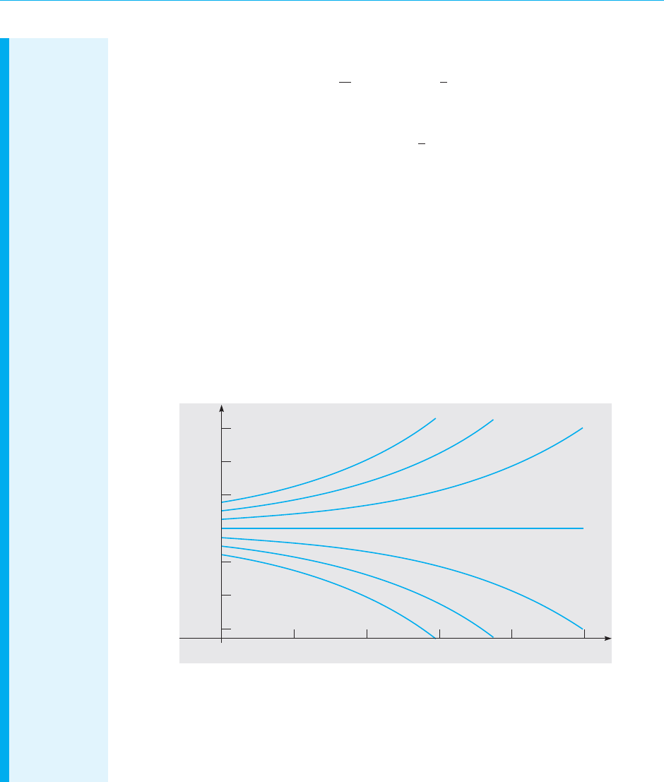
we show the equilibrium solution v(t) = 49 superimposed on the direction field. From this
figure we can draw another conclusion, namely, that all other solutions seem to be converging
to the equilibrium solution as t increases. Thus,in this context,the equilibrium solution is often
called the terminal velocity.
24 t6810
48
44
40
52
60
56
υ
FIGURE 1.1.2 A direction field for Eq. (5): d v/dt = 9.8 − (v/5).
24 t6810
48
44
40
52
60
56
υ
FIGURE 1.1.3 Direction field and equilibrium solution for Eq. (5): dv/dt = 9.8 − (v/5).
The approach illustrated in Example 2 can be applied equally well to the more
general Eq. (4), where the parameters m and γ are unspecified positive numbers.
The results are essentially identical to those of Example 2. The equilibrium solution
of Eq. (4) is v(t) = mg/γ. Solutions below the equilibriumsolution increasewith time,
those above it decrease with time, and all other solutions approach the equilibrium
solution as t becomes large.

August 7, 2012 21:03 c01 Sheet number 5 Page number 5 cyan black
1.1 Some Basic Mathematical Models; Direction Fields 5
Direction Fields. Direction fields are valuable tools in studying the solutions of
differential equations of the form
dy
dt
= f (t, y), (6)
where f is a given function of the two variables t and y, sometimes referred to as the
rate function. A direction field for equations of the form (6) can be constructed by
evaluating f at each point of a rectangular grid. At each point of the grid, a short line
segment is drawn whose slope is the value of f at that point. Thus each line segment
is tangent to the graph of the solution passing through that point. A direction field
drawn on a fairly fine grid gives a good picture of the overall behavior of solutions of
a differential equation. Usually a grid consisting of a few hundred points is sufficient.
The construction of a direction field is often a useful first step in the investigation of
a differential equation.
Two observations are worth particular mention. First, in constructing a direction
field, we do not have to solve Eq. (6); we just have to evaluate the given function
f (t, y) many times.Thus direction fields can be readily constructed even for equations
that may be quite difficult to solve. Second, repeated evaluation of a given function
is a task for which a computer is well suited, and you should usually use a computer
to draw a direction field. All the direction fields shown in this book, such as the one
in Figure 1.1.2, were computer-generated.
Field Mice and Owls. Now let us look at another, quite different example. Consider
a population of field mice who inhabit a certain rural area. In the absence of
predators we assume that the mouse population increases at a rate proportional
to the current population. This assumption is not a well-established physical law
(as Newton’s law of motion is in Example 1), but it is a common initial hypothesis
1
in a study of population growth. If we denote time by t and the mouse population by
p(t),then the assumption about population growth can be expressed by the equation
dp
dt
= rp, (7)
where the proportionality factor r is called the rate constant or growth rate.Tobe
specific,suppose that time is measured in months and that the rate constant r has the
value 0.5/month. Then each term in Eq. (7) has the units of mice/month.
Now let us add to the problem by supposing that several owls live in the same
neighborhood and that they kill 15 field mice per day.To incorporate this information
into the model, we must add another term to the differential equation (7), so that it
becomes
dp
dt
= 0.5p − 450. (8)
Observe that the predation term is −450 rather than −15 because time is measured
in months, so the monthly predation rate is needed.
1
A better model of population growth is discussed in Section 2.5.

August 7, 2012 21:03 c01 Sheet number 6 Page number 6 cyan black
6 Chapter 1. Intr oduction
EXAMPLE
3
Investigate the solutions of Eq. (8) graphically.
A direction field for Eq. (8) is shown in Figure 1.1.4. For sufficiently large values of p it can
be seen from the figure, or directly from Eq. (8) itself, that dp/dt is positive, so that solutions
increase. On the other hand, if p is small, then dp/dt is negative and solutions decrease. Again,
the critical value of p that separates solutions that increase from those that decrease is the
value of p for which dp/dt is zero. By setting dp/dt equal to zero in Eq. (8) and then solving
for p,we find the equilibrium solution p(t) = 900, for which the growth term and the predation
term in Eq. (8) are exactly balanced. The equilibrium solution is also shown in Figure 1.1.4.
12 t345
900
850
800
950
1000
p
FIGURE 1.1.4 Direction field and equilibrium solution for Eq. (8): dp/dt = 0.5p − 450.
Comparing Examples 2 and 3, we note that in both cases the equilibrium solution
separates increasing from decreasing solutions. In Example 2 other solutions con-
verge to, or are attracted by, the equilibrium solution, so that after the object falls far
enough, an observer will see it moving at very nearly the equilibrium velocity. On
the other hand, in Example 3 other solutions diverge from, or are repelled by, the
equilibrium solution. Solutions behave very differently depending on whether they
start above or below the equilibrium solution. As time passes, an observer might see
populations either much larger or much smaller than the equilibrium population,but
the equilibrium solution itself will not, in practice, be observed. In both problems,
however, the equilibrium solution is very important in understanding how solutions
of the given differential equation behave.
A more general version of Eq. (8) is
dp
dt
= rp − k, (9)
where the growth rate r and the predation rate k are unspecified. Solutions of this
more general equation are very similar to those of Eq. (8). The equilibrium solution
of Eq. (9) is p(t) = k /r. Solutions above the equilibrium solution increase, while
those below it decrease.
You should keep in mind that both of the models discussed in this section have
their limitations. The model (5) of the falling object is valid only as long as the

August 7, 2012 21:03 c01 Sheet number 7 Page number 7 cyan black
1.1 Some Basic Mathematical Models; Direction Fields 7
object is falling freely, without encountering any obstacles. The population model
(8) eventually predicts negative numbers of mice (if p < 900) or enormously large
numbers (ifp > 900). Both of thesepredictions areunrealistic,so this model becomes
unacceptable after a fairly short time interval.
Constructing Mathematical Models. In applying differential equations to any of the
numerous fields in which they are useful, it is necessary first to formulate the appro-
priate differential equation that describes,or models,the problem being investigated.
In this section we have looked at two examples of this modeling process, one drawn
from physics and the other from ecology. In constructing future mathematical mod-
els yourself, you should recognize that each problem is different, and that successful
modeling cannot be reduced to the observance of a set of prescribed rules. Indeed,
constructing a satisfactory model is sometimes the most difficult part of the problem.
Nevertheless, it may be helpful to list some steps that are often part of the process:
1. Identify the independent and dependent variables and assign letters to represent them.
Often the independent variable is time.
2. Choose the units of measurement for each variable. In a sense the choice of units is
arbitrary, but some choices may be much more convenient than others. For example, we
chose to measure time in seconds for the falling-object problem and in months for the
population problem.
3. Articulate the basic principle that underlies or governs the problem you are investigating.
This may be a widely recognized physical law,such as Newton’s law of motion,or it may be
a more speculative assumption that may be based on your own experience or observations.
In any case, this step is likely not to be a purely mathematical one, but will require you to
be familiar with the field in which the problem originates.
4. Express the principle or law in step 3 in terms of the variables you chose in step 1. This
may be easier said than done. It may require the introduction of physical constants or
parameters (such as the drag coefficient in Example 1) and the determination of appro-
priate values for them. Or it may involve the use of auxiliary or intermediate variables
that must then be related to the primary variables.
5. Make sure that all terms in your equation have the same physical units. If this is not the
case, then your equation is wrong and you should seek to repair it. If the units agree, then
your equation at least is dimensionally consistent,although it may have other shortcomings
that this test does not reveal.
6. In the problems considered here,the result of step 4 is a single differential equation,which
constitutes the desired mathematical model. Keep in mind, though, that in more complex
problems the resulting mathematical model may be much more complicated, perhaps
involving a system of several differential equations, for example.
PROBLEMS In each of Problems 1 through 6, draw a direction field for the given differential equation.
Based on the direction field, determine the behavior of y as t →∞. If this behavior depends
on the initial value of y at t = 0, describe the dependency.
1.
y
′
= 3 − 2y 2. y
′
= 2y − 3
3.
y
′
= 3 + 2y 4. y
′
=−1 − 2y
5.
y
′
= 1 + 2y 6. y
′
= y + 2

August 7, 2012 21:03 c01 Sheet number 8 Page number 8 cyan black
8 Chapter 1. Intr oduction
In each of Problems 7 through 10, write down a differential equation of the form
dy/dt = ay + b whose solutions have the required behavior as t →∞.
7. All solutions approach y = 3. 8. All solutions approach y = 2/3.
9. All other solutions diverge from y = 2. 10. All other solutions diverge from y = 1/3.
In each of Problems 11 through 14, draw a direction field for the given differential equation.
Based on the direction field, determine the behavior of y as t →∞. If this behavior depends
on the initial value of y at t = 0, describe this dependency. Note that in these problems the
equations are not of the form y
′
= ay + b, and the behavior of their solutions is somewhat
more complicated than for the equations in the text.
11.
y
′
= y(4 − y) 12. y
′
=−y(5 − y)
13.
y
′
= y
2
14. y
′
= y(y − 2)
2
Consider the following list of differential equations, some of which produced the direction
fields shown in Figures 1.1.5 through 1.1.10. In each of Problems 15 through 20 identify the
differential equation that corresponds to the given direction field.
(a) y
′
= 2y − 1 (b) y
′
= 2 + y (c) y
′
= y − 2
(d) y
′
= y(y + 3) (e) y
′
= y(y − 3) (f) y
′
= 1 + 2y
(g) y
′
=−2 − y (h) y
′
= y(3 − y) (i) y
′
= 1 − 2y
(j) y
′
= 2 − y
15. The direction field of Figure 1.1.5.
16. The direction field of Figure 1.1.6.
1
2
3
4
1234
y
t
FIGURE 1.1.5 Problem 15.
1
2
3
4
1234
y
t
FIGURE 1.1.6 Problem 16.
17. The direction field of Figure 1.1.7.
18. The direction field of Figure 1.1.8.
–4
–3
–2
–1
1234
y
t
FIGURE 1.1.7 Problem 17.
–4
–3
–2
–1
1234
y
t
FIGURE 1.1.8 Problem 18.

August 7, 2012 21:03 c01 Sheet number 9 Page number 9 cyan black
1.1 Some Basic Mathematical Models; Direction Fields 9
19. The direction field of Figure 1.1.9.
20. The direction field of Figure 1.1.10.
–1
1
2
3
4
5
1234
y
t
FIGURE 1.1.9 Problem 19.
–1
1
2
3
4
5
1234
y
t
FIGURE 1.1.10 Problem 20.
21. A pond initially contains 1,000,000 gal of water and an unknown amount of an undesirable
chemical. Water containing 0.01 g of this chemical per gallon flows into the pond at a rate
of 300 gal/h. The mixture flows out at the same rate, so the amount of water in the pond
remains constant.Assume that the chemical is uniformly distributed throughout the pond.
(a) Write a differential equation for the amount of chemical in the pond at any time.
(b) How much of the chemicalwill bein the pondafter a verylong time?Does this limiting
amount depend on the amount that was present initially?
22. A spherical raindrop evaporates at a rate proportional to its surface area. Write a
differential equation for the volume of the raindrop as a function of time.
23. Newton’s law of cooling states that the temperature of an object changes at a rate propor-
tional to the difference between the temperature of the object itself and the temperature
of its surroundings (the ambient air temperature in most cases). Suppose that the ambient
temperature is 70
◦
F and that the rate constant is 0.05 (min)
−1
.Write a differential equation
for the temperature of the object at any time. Note that the differential equation is the
same whether the temperature of the object is above or below the ambient temperature.
24. A certain drug is being administered intravenously to a hospital patient. Fluid containing
5 mg/cm
3
of the drug enters the patient’s bloodstream at a rate of 100 cm
3
/h. The drug is
absorbed by body tissues or otherwise leaves the bloodstream at a rate proportional to
the amount present, with a rate constant of 0.4 (h)
−1
.
(a) Assuming that the drug is always uniformly distributed throughout the bloodstream,
write a differential equation for the amount of the drug that is present in the bloodstream
at any time.
(b) How much of the drug is present in the bloodstream after a long time?
25.
For small, slowly falling objects, the assumption made in the text that the drag force
is proportional to the velocity is a good one. For larger, more rapidly falling objects, it is
more accurate to assume that the drag force is proportional to the square of the velocity.
2
(a) Write a differential equation for the velocity of a falling object of mass m if the mag-
nitude of the drag force is proportional to the square of the velocity and its direction is
opposite to that of the velocity.
2
See Lyle N. Long and Howard Weiss, “The Velocity Dependence of Aerodynamic Drag: A Primer for
Mathematicians,”American Mathematical Monthly 106 (1999), 2, pp. 127–135.

August 7, 2012 21:03 c01 Sheet number 10 Page number 10 cyan black
10 Chapter 1. Intr oduction
(b) Determine the limiting velocity after a long time.
(c) If m = 10 kg, find the drag coefficient so that the limiting velocity is 49 m/s.
(d) Using the data in part (c), draw a direction field and compare it with Figure 1.1.3.
In each of Problems 26 through 33, draw a direction field for the given differential equation.
Based on the direction field, determine the behavior of y as t →∞. If this behavior depends
on the initial value of y at t = 0, describe this dependency. Note that the right sides of these
equations depend on t as well as y; therefore, their solutions can exhibit more complicated
behavior than those in the text.
26.
y
′
=−2 + t − y 27. y
′
= te
−2t
− 2y
28.
y
′
= e
−t
+ y 29. y
′
= t + 2y
30.
y
′
= 3 sin t + 1 + y 31. y
′
= 2t − 1 − y
2
32. y
′
=−(2t + y)/2y 33. y
′
=
1
6
y
3
− y −
1
3
t
2
1.2 Solutions of Some Differential Equations
In the preceding section we derived the differential equations
m
d v
dt
= mg − γv (1)
and
dp
dt
= rp − k. (2)
Equation (1) models a falling object, and Eq. (2) models a population of field mice
preyed on by owls. Both of these equations are of the general form
dy
dt
= ay − b, (3)
where a and b are given constants. We were able to draw some important qualitative
conclusions about the behavior of solutions of Eqs. (1) and (2) by considering the
associated direction fields. To answer questions of a quantitative nature,however,we
need to find the solutions themselves, and we now investigate how to do that.
EXAMPLE
1
Fiel d Mi ce
and Owls
(continued)
Consider the equation
dp
dt
= 0.5p − 450, (4)
which describes the interaction of certain populations of field mice and owls [see Eq. (8) of
Section 1.1]. Find solutions of this equation.
To solve Eq. (4), we need to find functions p(t) that, when substituted into the equation,
reduce it to an obvious identity. Here is one way to proceed. First, rewrite Eq. (4) in the form
dp
dt
=
p − 900
2
, (5)
or, if p ̸= 900,
dp/dt
p − 900
=
1
2
. (6)
August 7, 2012 21:03 c01 Sheet number 11 Page number 11 cyan black
1.2 Solutions of Some Differential Equations 11
By the chain rule the left side of Eq. (6) is the derivative of ln |p − 900| with respect to t,sowe
have
d
dt
ln |p − 900|=
1
2
. (7)
Then, by integrating both sides of Eq. (7), we obtain
ln |p − 900|=
t
2
+ C, (8)
where C is an arbitrary constant of integration. Therefore, by taking the exponential of both
sides of Eq. (8), we find that
|p − 900|=e
(t/2)+C
= e
C
e
t/2
, (9)
or
p − 900 =±e
C
e
t/2
, (10)
and finally
p = 900 + ce
t/2
, (11)
where c =±e
C
is also an arbitrary (nonzero) constant. Note that the constant function p = 900
is also a solution of Eq. (5) and that it is contained in the expression (11) if we allow c to take
the value zero. Graphs of Eq. (11) for several values of c are shown in Figure 1.2.1.
900
600
12 t345
700
800
1000
1100
1200
p
FIGURE 1.2.1 Graphs of p = 900 + ce
t/2
for several values of c.
These are solutions of dp/dt = 0.5p − 450.
Note that they have the character inferred from the direction field in Figure 1.1.4. For
instance, solutions lying on either side of the equilibrium solution p = 900 tend to diverge
from that solution.
In Example 1 we found infinitely many solutions of the differential equation (4),
corresponding to the infinitely many values that the arbitrary constant c in Eq. (11)
might have.Thisis typicalof what happenswhen yousolve adifferential equation.The
solution process involves an integration, which brings with it an arbitrary constant,
whose possible values generate an infinite family of solutions.

August 7, 2012 21:03 c01 Sheet number 12 Page number 12 cyan black
12 Chapter 1. Intr oduction
Frequently,we want to focus our attention on a single member of the infinite family
of solutions by specifying the value of the arbitrary constant. Most often, we do this
indirectly by specifying instead a point that must lie on the graph of the solution. For
example,to determine the constant c in Eq. (11),we could require that the population
have a given value at a certain time,such as the value 850 at time t = 0. In other words,
the graph of the solution must pass through the point (0, 850). Symbolically, we can
express this condition as
p(0) = 850. (12)
Then, substituting t = 0 and p = 850 into Eq. (11), we obtain
850 = 900 + c.
Hence c =−50, and by inserting this value into Eq. (11), we obtain the desired
solution, namely,
p = 900 − 50e
t/2
. (13)
The additional condition (12) that we used to determine c is an example of an
initial condition. The differential equation (4) together with the initial condition (12)
form an initial value problem.
Now consider the more general problem consisting of the differential equation (3)
dy
dt
= ay − b
and the initial condition
y(0) = y
0
, (14)
where y
0
is an arbitrary initial value. We can solve this problem by the same method
as in Example 1. If a ̸= 0 and y ̸= b/a, then we can rewrite Eq. (3) as
dy/dt
y − (b/a)
= a. (15)
By integrating both sides, we find that
ln |y − (b/a)|=at + C, (16)
where C is arbitrary.Then,taking the exponential ofboth sidesof Eq.(16) and solving
for y, we obtain
y = (b/a) + ce
at
, (17)
where c =±e
C
is also arbitrary. Observe that c = 0 corresponds to the equilibrium
solution y = b/a. Finally, the initial condition (14) requires that c = y
0
− (b/a), so
the solution of the initial value problem (3), (14) is
y = (b/a) +[y
0
− (b/a)]e
at
. (18)
For a ̸= 0 the expression (17) contains all possible solutions of Eq. (3) and is called
the general solution.
3
The geometrical representation of the general solution (17) is
an infinite family of curves called integral curves. Each integral curve is associated
with a particular value of c and is the graph of the solution corresponding to that
3
If a = 0,then the solution of Eq. (3) is not given by Eq. (17). We leave it to you to find the general solution
in this case.

August 7, 2012 21:03 c01 Sheet number 13 Page number 13 cyan black
1.2 Solutions of Some Differential Equations 13
value of c. Satisfying an initial condition amounts to identifying the integral curve
that passes through the given initial point.
To relate the solution (18) to Eq. (2), which models the field mouse population, we
need only replace a by the growth rate r and replace b by the predation rate k. Then
the solution (18) becomes
p = (k/r) +[p
0
− (k/r)]e
rt
, (19)
where p
0
is the initial population of field mice. The solution (19) confirms the conclu-
sions reached on the basis of the direction field and Example 1. If p
0
= k/r,then from
Eq. (19) it follows that p = k/r for all t; this is the constant, or equilibrium, solution.
If p
0
̸= k /r, then the behavior of the solution depends on the sign of the coefficient
p
0
− (k/r) of theexponential term in Eq. (19). If p
0
> k/r,then p grows exponentially
with time t;ifp
0
< k/r,then p decreases and eventually becomes zero, corresponding
to extinction of the field mouse population. Negative values of p, while possible for
the expression (19), make no sense in the context of this particular problem.
To put the falling-object equation (1) in the form (3),we must identify a with −γ/m
and b with −g. Making these substitutions in the solution (18), we obtain
v = (mg/γ) +[v
0
− (mg/γ)]e
−γt/m
, (20)
where v
0
is the initial velocity. Again, this solution confirms the conclusions reached
in Section 1.1 on the basis of a direction field. There is an equilibrium, or constant,
solution v = mg/γ,and all other solutions tend to approach this equilibrium solution.
The speed of convergence to the equilibrium solution is determined by the exponent
−γ/m. Thus, for a given mass m, the velocity approaches the equilibrium value more
rapidly as the drag coefficient γ increases.
EXAMPLE
2
AFalling
Object
(continued)
Suppose that, as in Example 2 of Section 1.1, we consider a falling object of mass m = 10 kg
and drag coefficient γ = 2 kg/s. Then the equation of motion (1) becomes
dv
dt
= 9.8 −
v
5
. (21)
Suppose this object is dropped from a height of 300 m. Find its velocity at any time t. How
long will it take to fall to the ground, and how fast will it be moving at the time of impact?
The first step is to state an appropriate initial condition for Eq. (21). The word “dropped” in
the statement of the problem suggests that the initial velocity is zero, so we will use the initial
condition
v(0) = 0. (22)
The solution of Eq. (21) can be found by substituting the values of the coefficients into the
solution (20),but we will proceed instead to solve Eq. (21) directly. First,rewrite the equation as
dv/dt
v − 49
=−
1
5
. (23)
By integrating both sides, we obtain
ln |v − 49|=−
t
5
+ C, (24)
and then the general solution of Eq. (21) is
v = 49 + ce
−t/5
, (25)

August 7, 2012 21:03 c01 Sheet number 14 Page number 14 cyan black
14 Chapter 1. Intr oduction
where c is arbitrary. To determine c, we substitute t = 0 and v = 0 from the initial condition
(22) into Eq. (25), with the result that c =−49. Then the solution of the initial value problem
(21), (22) is
v = 49(1 − e
−t/5
). (26)
Equation (26) gives the velocity of the falling object at any positive time (before it hits the
ground, of course).
Graphs of the solution (25) for several values of c are shown in Figure 1.2.2,with the solution
(26) shown by the black curve. It is evident that all solutions tend to approach the equilibrium
solution v = 49. This confirms the conclusions we reached in Section 1.1 on the basis of the
direction fields in Figures 1.1.2 and 1.1.3.
100
80
60
40
20
24 t6 8 1210
v
v = 49 (1 – e
–t/5
)
(10.51, 43.01)
FIGURE 1.2.2 Graphs of the solution (25), v = 49 + ce
−t/5
, for several
values of c. The black curve corresponds to the initial condition v(0) = 0.
To find the velocity of the object when it hits the ground, we need to know the time at which
impact occurs. In other words, we need to determine how long it takes the object to fall 300 m.
To do this, we note that the distance x the object has fallen is related to its velocity v by the
equation v = dx/dt, or
dx
dt
= 49(1 − e
−t/5
). (27)
Consequently, by integrating both sides of Eq. (27), we have
x = 49t + 245e
−t/5
+ c, (28)
where c is an arbitrary constant of integration. The object starts to fall when t = 0, so we know
that x = 0 when t = 0. From Eq. (28) it follows that c =−245, so the distance the object has
fallen at time t is given by
x = 49t + 245e
−t/5
− 245. (29)
Let T be the time at which the object hits the ground;then x = 300 when t = T. By substituting
these values in Eq. (29), we obtain the equation
49T + 245e
−T/5
− 545 = 0. (30)

August 7, 2012 21:03 c01 Sheet number 15 Page number 15 cyan black
1.2 Solutions of Some Differential Equations 15
Thevalue of T satisfying Eq. (30) can be approximated by a numerical process
4
using a scientific
calculator or computer,withthe resultthat T
∼
=
10.51 s.At this time,the corresponding velocity
v
T
is found from Eq. (26) to be v
T
∼
=
43.01 m/s. The point (10.51, 43.01) is also shown in
Figure 1.2.2.
Further Remarks on Mathematical Modeling. Up to this point we have related our discus-
sion of differential equations to mathematical models of a falling object and of a
hypothetical relation between field mice and owls. The derivation of these models
may have been plausible, and possibly even convincing, but you should remember
that the ultimate test of any mathematical model is whether its predictions agree
with observations or experimental results. We have no actual observations or exper-
imental results to use for comparison purposes here, but there are several sources of
possible discrepancies.
In the case of the falling object, the underlying physical principle (Newton’s law
of motion) is well established and widely applicable. However, the assumption that
the drag force is proportional to the velocity is less certain. Even if this assumption is
correct, the determination of the drag coefficient γ by direct measurement presents
difficulties. Indeed, sometimes one finds the drag coefficient indirectly—for example,
by measuring the time of fall from a given height and then calculating the value of γ
that predicts this observed time.
The model of the field mouse population is subject to various uncertainties.
The determination of the growth rate r and the predation rate k depends on
observations of actual populations, which may be subject to considerable variation.
The assumption that r and k are constants may also be questionable. For example,
a constant predation rate becomes harder to sustain as the field mouse population
becomes smaller. Further, the model predicts that a population above the equilib-
rium value will grow exponentially larger and larger. This seems at variance with the
behavior of actual populations; see the further discussion of population dynamics in
Section 2.5.
If the differences between actual observations and a mathematical model’s pre-
dictions are too great, then you need to consider refining the model, making more
careful observations, or perhaps both. There is almost always a tradeoff between
accuracy and simplicity. Both are desirable, but a gain in one usually involves a loss
in the other. However,even if a mathematical model is incomplete or somewhat inac-
curate,it may nevertheless be useful in explaining qualitative features of the problem
under investigation. It may also give satisfactory results under some circumstances
but not others. Thus you should always use good judgment and common sense in
constructing mathematical models and in using their predictions.
PROBLEMS 1.
Solve each of the following initial value problems and plot the solutions for several values
of y
0
. Then describe in a few words how the solutions resemble, and differ from, each
other.
(a) dy/dt =−y + 5, y(0) = y
0
4
A computer algebra system provides this capability; many calculators also have built-in routines for
solving such equations.

August 7, 2012 21:03 c01 Sheet number 16 Page number 16 cyan black
16 Chapter 1. Intr oduction
(b) dy/dt =−2y + 5, y(0) = y
0
(c) dy/dt =−2y + 10, y(0) = y
0
2. Follow the instructions for Problem 1 for the following initial value problems:
(a) dy/dt = y − 5, y(0) = y
0
(b) dy/dt = 2y − 5, y(0) = y
0
(c) dy/dt = 2y − 10, y(0) = y
0
3. Consider the differential equation
dy/dt =−ay + b,
where both a and b are positive numbers.
(a) Find the general solution of the differential equation.
(b) Sketch the solution for several different initial conditions.
(c) Describe how the solutions change under each of the following conditions:
i. a increases.
ii. b increases.
iii. Both a and b increase, but the ratio b/a remains the same.
4. Consider the differential equation dy/dt = ay − b.
(a) Find the equilibrium solution y
e
.
(b) Let Y(t) = y − y
e
; thus Y(t) is the deviation from the equilibrium solution. Find the
differential equation satisfied by Y(t).
5. Undetermined Coefficients. Here is an alternative way to solve the equation
dy/dt = ay − b. (i)
(a) Solve the simpler equation
dy/dt = ay. (ii)
Call the solution y
1
(t).
(b) Observe that the only difference between Eqs. (i) and (ii) is the constant −b in Eq. (i).
Therefore, it may seem reasonable to assume that the solutions of these two equations
also differ only by a constant. Test this assumption by trying to find a constant k such that
y = y
1
(t) + k is a solution of Eq. (i).
(c) Compare your solution from part (b) with the solution given in the text in Eq. (17).
Note: This method can also be used in some cases in which the constant b is replaced
by a function g(t). It depends on whether you can guess the general form that the solution
is likely to take.This method is described in detail in Section 3.5 in connection with second
order equations.
6. Use the method of Problem 5 to solve the equation
dy/dt =−ay + b.
7. The field mouse population in Example 1 satisfies the differential equation
dp/dt = 0.5p − 450.
(a) Find the time at which the population becomes extinct if p(0) = 850.
(b) Find the time of extinction if p(0) = p
0
, where 0 < p
0
< 900.
(c) Find the initial population p
0
if the population is to become extinct in 1 year.

August 7, 2012 21:03 c01 Sheet number 17 Page number 17 cyan black
1.2 Solutions of Some Differential Equations 17
8. Consider a population p of field mice that grows at a rate proportional to the current
population, so that dp/dt = rp.
(a) Find the rate constant r if the population doubles in 30 days.
(b) Find r if the population doubles in N days.
9. The falling object in Example 2 satisfies the initial value problem
dv/dt = 9.8 − (v/5), v(0) = 0.
(a) Find the time that must elapse for the object to reach 98% of its limiting velocity.
(b) How far does the object fall in the time found in part (a)?
10. Modify Example 2 so that the falling object experiences no air resistance.
(a) Write down the modified initial value problem.
(b) Determine how long it takes the object to reach the ground.
(c) Determine its velocity at the time of impact.
11.
Consider the falling object of mass 10 kg in Example 2,but assume now that the drag force
is proportional to the square of the velocity.
(a) If the limiting velocity is 49 m/s (the same as in Example 2), show that the equation
of motion can be written as
dv/dt =[(49)
2
− v
2
]/245.
Also see Problem 25 of Section 1.1.
(b) If v(0) = 0, find an expression for v(t) at any time.
(c) Plot your solution from part (b) and the solution (26) from Example 2 on the same
axes.
(d) Based on your plots in part (c), compare the effect of a quadratic drag force with that
of a linear drag force.
(e) Find the distance x (t) that the object falls in time t.
(f) Find the time T it takes the object to fall 300 m.
12. A radioactive material,suchas the isotope thorium-234,disintegratesat a rate proportional
to the amount currently present.If Q(t) is the amount presentat time t,then dQ/dt =−rQ,
where r > 0 is the decay rate.
(a) If 100 mg of thorium-234 decays to 82.04 mg in 1 week, determine the decay rate r.
(b) Find an expression for the amount of thorium-234 present at any time t.
(c) Find the time required for the thorium-234 to decay to one-half its original amount.
13. The half-life of a radioactive material is the time required for an amount of this material
to decay to one-half its original value. Show that for any radioactive material that decays
according to the equation Q
′
=−rQ,the half-lifeτ and the decay rate r satisfy the equation
rτ = ln 2.
14. Radium-226 has a half-life of 1620 years. Find the time period during which a given amount
of this material is reduced by one-quarter.
15. According to Newton’s law of cooling (see Problem 23 of Section 1.1), the temperature
u(t) of an object satisfies the differential equation
du
dt
=−k(u − T),
where T is the constant ambient temperature and k is a positive constant. Suppose that
the initial temperature of the object is u(0) = u
0
.
(a) Find the temperature of the object at any time.

August 7, 2012 21:03 c01 Sheet number 18 Page number 18 cyan black
18 Chapter 1. Intr oduction
(b) Let τ be the time at which the initial temperature difference u
0
− T has been reduced
by half. Find the relation between k and τ.
16. Supposethat a building loses heatin accordance with Newton’slaw ofcooling (see Problem
15)and that the rate constantk hasthevalue 0.15h
−1
.Assume thatthe interior temperature
is 70
◦
F when the heating system fails. If the external temperature is 10
◦
F, how long will it
take for the interior temperature to fall to 32
◦
F?
17. Consider an electric circuit containing a capacitor, resistor, and battery; see Figure 1.2.3.
The charge Q(t) on the capacitor satisfies the equation
5
R
dQ
dt
+
Q
C
= V,
where R is the resistance, C is the capacitance, and V is the constant voltage supplied by
the battery.
(a) If Q(0) = 0, find Q(t) at any time t, and sketch the graph of Q versus t.
(b) Find the limiting value Q
L
that Q(t) approaches after a long time.
(c) Suppose that Q(t
1
) = Q
L
and that at time t = t
1
the battery is removed and the circuit
is closed again. Find Q(t) for t > t
1
and sketch its graph.
V
R
C
FIGURE 1.2.3 The electric circuit of Problem 17.
18.
A pond containing 1,000,000 gal of water is initially free of a certain undesirable chemical
(see Problem 21 of Section 1.1). Water containing 0.01 g/gal of the chemical flows into the
pond at a rate of 300 gal/h, and water also flows out of the pond at the same rate. Assume
that the chemical is uniformly distributed throughout the pond.
(a) Let Q(t) be the amount of the chemical in the pond at time t. Write down an initial
value problem for Q(t).
(b) Solve the problem in part (a) for Q(t). How much chemical is in the pond after 1 year?
(c) At the end of 1 year the source of the chemical in the pond is removed; thereafter
pure water flows into the pond, and the mixture flows out at the same rate as before.Write
down the initial value problem that describes this new situation.
(d) Solve the initial value problem in part (c). How much chemical remains in the pond
after 1 additional year (2 years from the beginning of the problem)?
(e) How long does it take for Q(t) to be reduced to 10 g?
(f) Plot Q(t) versus t for 3 years.
19. Your swimming pool containing 60,000 gal of water has been contaminated by 5 kg of
a nontoxic dye that leaves a swimmer’s skin an unattractive green. The pool’s filtering
system can take water from the pool, remove the dye, and return the water to the pool at
a flow rate of 200 gal/min.
5
This equation results from Kirchhoff’s laws, which are discussed in Section 3.7.

August 7, 2012 21:03 c01 Sheet number 19 Page number 19 cyan black
1.3 Classification of Differential Equations 19
(a) Write down the initial value problem for the filtering process; let q(t) be the amount
of dye in the pool at any time t.
(b) Solve the problem in part (a).
(c) You have invited several dozen friends to a pool party that is scheduled to begin in 4 h.
You have also determined that the effect of the dye is imperceptible if its concentration
is less than 0.02 g/gal. Is your filtering system capable of reducing the dye concentration
to this level within 4 h?
(d) Find the time T at which the concentration of dye first reaches the value 0.02 g/gal.
(e) Find the flow rate that is sufficient to achieve the concentration 0.02 g/gal within 4 h.
1.3 Classification of Differential Equations
The main purpose of this book is to discuss some of the properties of solutions of
differential equations,and to present some of the methods that have proved effective
in finding solutions or, in some cases, approximating them. To provide a framework
for our presentation, we describe here several useful ways of classifying differential
equations.
Ordinar y and Partial Differential Equations. One important classification is based on
whether the unknown function depends on a single independent variable or on sev-
eral independent variables. In the first case, only ordinary derivatives appear in the
differential equation, and it is said to be an ordinary differential equation. In the sec-
ond case, the derivatives are partial derivatives, and the equation is called a partial
differential equation.
All the differential equations discussed in the preceding two sections are ordinary
differential equations. Another example of an ordinary differential equation is
L
d
2
Q(t)
dt
2
+ R
dQ(t)
dt
+
1
C
Q(t) = E(t), (1)
for the charge Q(t) on a capacitor in a circuit with capacitance C, resistance R, and
inductance L; this equation is derived in Section 3.7. Typical examples of partial
differential equations are the heat conduction equation
α
2
∂
2
u(x, t)
∂x
2
=
∂u(x, t)
∂t
(2)
and the wave equation
a
2
∂
2
u(x, t)
∂x
2
=
∂
2
u(x, t)
∂t
2
. (3)
Here, α
2
and a
2
are certain physical constants. Note that in both Eqs. (2) and (3) the
dependent variable u depends on the two independent variables x and t. The heat
conduction equation describes the conduction of heat in a solid body, and the wave
equation arises in a variety of problems involving wave motion in solids or fluids.
Systems of Differential Equations. Another classification of differential equations de-
pends on the number of unknown functions that are involved. If there is a single

August 7, 2012 21:03 c01 Sheet number 20 Page number 20 cyan black
20 Chapter 1. Intr oduction
function to be determined, then one equation is sufficient. However, if there are two
or more unknown functions, then a system of equations is required. For example, the
Lotka–Volterra, or predator–prey, equations are important in ecological modeling.
They have the form
dx/dt = ax − αxy
dy/dt =−cy + γxy,
(4)
where x(t) and y(t) are the respective populations of the prey and predator species.
The constants a, α, c, and γ are based on empirical observations and depend on the
particular species being studied. Systems of equations are discussed in Chapters 7
and 9; in particular, the Lotka–Volterra equations are examined in Section 9.5. In
some areas of application it is not unusual to encounter very large systems containing
hundreds, or even many thousands, of equations.
Order. The order of a differential equation is the order of the highest derivative that
appears in the equation. The equations in the preceding sections are all first order
equations, whereas Eq. (1) is a second order equation. Equations (2) and (3) are
second order partial differential equations. More generally, the equation
F[t, u(t), u
′
(t), ..., u
(n)
(t)]=0 (5)
is an ordinary differential equation of the nth order. Equation (5) expresses a relation
between the independent variable t and the values of the function u and its first n
derivatives u
′
, u
′′
, ..., u
(n)
. It is convenient and customary in differential equations to
write y for u(t), with y
′
, y
′′
, ..., y
(n)
standing for u
′
(t), u
′′
(t), ..., u
(n)
(t). Thus Eq. (5) is
written as
F(t, y, y
′
, ..., y
(n)
) = 0. (6)
For example,
y
′′′
+ 2e
t
y
′′
+ yy
′
= t
4
(7)
is a third order differential equation for y = u(t). Occasionally, other letters will be
used instead of t and y for the independent and dependent variables; the meaning
should be clear from the context.
We assume that it is always possible to solve a given ordinary differential equation
for the highest derivative, obtaining
y
(n)
= f (t, y, y
′
, y
′′
, ..., y
(n−1)
). (8)
This is mainly to avoid the ambiguity that may arise because a single equation of
the form (6) may correspond to several equations of the form (8). For example, the
equation
(y
′
)
2
+ ty
′
+ 4y = 0 (9)
leads to the two equations
y
′
=
−t +
!
t
2
− 16y
2
or y
′
=
−t −
!
t
2
− 16y
2
. (10)
Linear and Nonlinear Equations. A crucial classification of differential equations is
whether they are linear or nonlinear. The ordinary differential equation
F(t, y, y
′
, ..., y
(n)
) = 0

August 7, 2012 21:03 c01 Sheet number 21 Page number 21 cyan black
1.3 Classification of Differential Equations 21
is said to be linear if F is a linear function of the variables y, y
′
, ..., y
(n)
; a similar
definition applies to partial differential equations. Thus the general linear ordinary
differential equation of order n is
a
0
(t)y
(n)
+ a
1
(t)y
(n−1)
+···+a
n
(t)y = g(t). (11)
Most of the equations you have seen thus far in this book are linear; examples are
the equations in Sections 1.1 and 1.2 describing the falling object and the field mouse
population. Similarly, in this section, Eq. (1) is a linear ordinary differential equation
and Eqs. (2) and (3) are linear partial differential equations. An equation that is not
of the form (11) is a nonlinear equation. Equation (7) is nonlinear because of the
term yy
′
. Similarly, each equation in the system (4) is nonlinear because of the terms
that involve the product xy.
A simple physical problem that leads to a nonlinear differential equation is the
oscillating pendulum. The angle θ that an oscillating pendulum of length L makes
with the vertical direction (see Figure 1.3.1) satisfies the equation
d
2
θ
dt
2
+
g
L
sin θ = 0, (12)
whose derivation is outlined in Problems 29 through 31. The presence of the term
involving sin θ makes Eq. (12) nonlinear.
L
m
mg
θ
FIGURE 1.3.1 An oscillating pendulum.
The mathematical theory and methods for solving linear equations are highly
developed. In contrast, for nonlinear equations the theory is more complicated, and
methods of solution are less satisfactory. In view of this, it is fortunate that many
significant problems lead to linear ordinary differential equations or can be approx-
imated by linear equations. For example, for the pendulum, if the angle θ is small,
then sin θ
∼
=
θ and Eq. (12) can be approximated by the linear equation
d
2
θ
dt
2
+
g
L
θ = 0. (13)
This process of approximating a nonlinear equation by a linear one is called lineariza-
tion; it is an extremely valuable way to deal with nonlinear equations. Nevertheless,
there are many physical phenomena that simply cannot be represented adequately
by linear equations. To study these phenomena, it is essential to deal with nonlinear
equations.

August 7, 2012 21:03 c01 Sheet number 22 Page number 22 cyan black
22 Chapter 1. Intr oduction
In an elementary text it is natural to emphasize the simpler and more straight-
forward parts of the subject. Therefore, the greater part of this book is devoted to
linear equations and various methods for solving them. However, Chapters 8 and 9,
as well as parts of Chapter 2, are concerned with nonlinear equations. Whenever it
is appropriate, we point out why nonlinear equations are, in general, more difficult
and why many of the techniques that are useful in solving linear equations cannot
be applied to nonlinear equations.
Solutions. A solution of the ordinary differential equation (8) on the interval
α<t <βis a function φ such that φ
′
, φ
′′
, ..., φ
(n)
exist and satisfy
φ
(n)
(t) = f [t, φ(t), φ
′
(t), ..., φ
(n−1)
(t)] (14)
for every t in α<t <β. Unless stated otherwise, we assume that the function f
of Eq. (8) is a real-valued function, and we are interested in obtaining real-valued
solutions y = φ(t).
Recall that in Section 1.2 we found solutions of certain equations by a process of
direct integration. For instance, we found that the equation
dp
dt
= 0.5p − 450 (15)
has the solution
p = 900 + ce
t/2
, (16)
where c is an arbitrary constant. It is often not so easy to find solutions of differential
equations. However, if you find a function that you think may be a solution of a given
equation, it is usually relatively easy to determine whether the function is actually a
solution simply by substituting the function into the equation. For example, in this
way it is easy to show that the function y
1
(t) = cos t is a solution of
y
′′
+ y = 0 (17)
for all t.To confirm this, observe that y
′
1
(t) =−sin t and y
′′
1
(t) =−cos t;then it follows
that y
′′
1
(t) + y
1
(t) = 0. In the same way you can easily show that y
2
(t) = sin t is also
a solution of Eq. (17). Of course, this does not constitute a satisfactory way to solve
most differential equations,because there are far too many possible functions for you
to have a good chance of finding the correct one by a random choice. Nevertheless,
you should realize that you can verify whether any proposed solution is correct by
substituting it into the differential equation. This can be a very useful check; it is one
that you should make a habit of considering.
Some Important Questions. Although for the equations (15) and (17) we are able to
verify that certain simple functions are solutions, in general we do not have such
solutions readily available. Thus a fundamental question is the following: Does an
equation of the form (8) always have a solution? The answer is “No.” Merely writing
down an equation of the form (8) does not necessarily mean that there is a function
y = φ(t) that satisfies it. So, how can we tell whether some particular equation has a
solution?This is the question of existence of a solution,and it is answered by theorems
stating that under certain restrictions on the function f in Eq. (8),the equation always
has solutions. This is not a purely mathematical concern for at least two reasons.

August 7, 2012 21:03 c01 Sheet number 23 Page number 23 cyan black
1.3 Classification of Differential Equations 23
If a problem has no solution, we would prefer to know that fact before investing
time and effort in a vain attempt to solve the problem. Further, if a sensible physical
problem is modeled mathematically as a differential equation, then the equation
should have a solution. If it does not,then presumably there is something wrong with
the formulation. In this sense an engineer or scientist has some check on the validity
of the mathematical model.
If we assume that a given differential equation has at least one solution, then
we may need to consider how many solutions it has, and what additional conditions
must be specified to single out aparticular solution.This is the question ofuniqueness.
In general, solutions of differential equations contain one or more arbitrary con-
stants of integration, as does the solution (16) of Eq. (15). Equation (16) represents
an infinity of functions corresponding to the infinity of possible choices of the con-
stant c. As we saw in Section 1.2, if p is specified at some time t, this condition will
determine a value for c; even so, we have not yet ruled out the possibility that there
may be other solutions of Eq. (15) that also have the prescribed value of p at the
prescribed time t. As in the question of existence of solutions, the issue of uniqueness
has practical as well as theoretical implications. If we are fortunate enough to find a
solution of a given problem, and if we know that the problem has a unique solution,
then we can be sure that we have completely solved the problem. If there may be
other solutions, then perhaps we should continue to search for them.
A third important question is: Given a differential equation of the form (8), can
we actually determine a solution, and if so, how? Note that if we find a solution of
the given equation, we have at the same time answered the question of the exis-
tence of a solution. However, without knowledge of existence theory we might,
for example, use a computer to find a numerical approximation to a “solution”
that does not exist. On the other hand, even though we may know that a solution
exists, it may be that the solution is not expressible in terms of the usual elemen-
tary functions—polynomial, trigonometric, exponential, logarithmic, and hyperbolic
functions. Unfortunately, this is the situation for most differential equations. Thus,
we discuss both elementary methods that can be used to obtain exact solutions of
certain relatively simple problems, and also methods of a more general nature that
can be used to find approximations to solutions of more difficult problems.
Computer Use in Differential Equations. A computer can be an extremely valuable tool
in the study of differential equations. For many years computers have been used
to execute numerical algorithms, such as those described in Chapter 8, to construct
numerical approximations to solutions of differential equations. These algorithms
have been refined to an extremely high level of generality and efficiency. A few lines
of computer code,written in a high-level programming language and executed (often
within a few seconds) on a relatively inexpensive computer,suffice to approximate to
a high degree of accuracy thesolutions of a wide rangeof differential equations. More
sophisticated routines are also readily available. These routines combine the ability
to handle very large and complicated systems with numerous diagnostic features that
alert the user to possible problems as they are encountered.
The usual output from a numerical algorithm is a table of numbers, listing selected
values of the independent variable and the corresponding values of the dependent
variable. With appropriate software it is easy to display the solution of a differen-
tial equation graphically, whether the solution has been obtained numerically or as

August 7, 2012 21:03 c01 Sheet number 24 Page number 24 cyan black
24 Chapter 1. Intr oduction
the result of an analytical procedure of some kind. Such a graphical display is often
much more illuminating and helpful in understanding and interpreting the solution of
a differential equation than a table of numbers or a complicated analytical formula.
There are on the market several well-crafted and relatively inexpensive special-
purpose software packages for the graphical investigation of differential equations.
The widespread availability of personal computers has brought powerful computa-
tional and graphical capability within the reach of individual students. You should
consider, in the light of your own circumstances, how best to take advantage of the
available computing resources. You will surely find it enlightening to do so.
Another aspect of computer use that is very relevant to the study of differential
equations is the availability of extremely powerful and general software packages
that can perform a wide variety of mathematical operations.Among these are Maple,
Mathematica,and MATLAB, each of which can be used on various kinds of personal
computers or workstations.All three of these packages can execute extensive numer-
ical computationsand haveversatile graphicalfacilities. Maple and Mathematica also
have very extensive analytical capabilities. For example, they can perform the ana-
lytical steps involved in solving many differential equations, often in response to a
single command. Anyone who expects to deal with differential equations in more
than a superficial way should become familiar with at least one of these products and
explore the ways in which it can be used.
For you, the student, these computing resources have an effect on how you should
study differential equations. To become confident in using differential equations, it
is essential to understand how the solution methods work, and this understanding is
achieved, in part,by working out a sufficient number of examples in detail. However,
eventually you should plan to delegate as many as possible of the routine (often
repetitive) details to a computer, while you focus on the proper formulation of the
problem and on the interpretation of the solution. Our viewpoint is that you should
always try to use the best methods and tools available for each task. In particular,
you should strive to combine numerical, graphical, and analytical methods so as to
attain maximum understanding of the behavior of the solution and of the underlying
process that the problem models.You should also remember that some tasks can best
be done with pencil and paper, while others require a calculator or computer. Good
judgment is often needed in selecting an effective combination.
PROBLEMS In each of Problems 1 through 6, determine the order of the given differential equation; also
state whether the equation is linear or nonlinear.
1. t
2
d
2
y
dt
2
+ t
dy
dt
+ 2y = sin t 2. (1 + y
2
)
d
2
y
dt
2
+ t
dy
dt
+ y = e
t
3.
d
4
y
dt
4
+
d
3
y
dt
3
+
d
2
y
dt
2
+
dy
dt
+ y = 14.
dy
dt
+ ty
2
= 0
5.
d
2
y
dt
2
+ sin(t + y) = sin t 6.
d
3
y
dt
3
+ t
dy
dt
+ (cos
2
t)y = t
3
In each of Problems 7 through 14, verify that each given function is a solution of the differ-
ential equation.
7. y
′′
− y = 0; y
1
(t) = e
t
, y
2
(t) = cosh t

August 7, 2012 21:03 c01 Sheet number 25 Page number 25 cyan black
1.3 Classification of Differential Equations 25
8. y
′′
+ 2y
′
− 3y = 0; y
1
(t) = e
−3t
, y
2
(t) = e
t
9. ty
′
− y = t
2
; y = 3t + t
2
10. y
′′′′
+ 4y
′′′
+ 3y = t; y
1
(t) = t/3, y
2
(t) = e
−t
+ t/3
11. 2t
2
y
′′
+ 3ty
′
− y = 0, t > 0; y
1
(t) = t
1/2
, y
2
(t) = t
−1
12. t
2
y
′′
+ 5ty
′
+ 4y = 0, t > 0; y
1
(t) = t
−2
, y
2
(t) = t
−2
ln t
13. y
′′
+ y = sec t,0< t <π/2; y = (cos t) ln cos t + t sin t
14. y
′
− 2ty = 1; y = e
t
2
"
t
0
e
−s
2
ds + e
t
2
In each of Problems 15 through 18, determine the values of r for which the given differential
equation has solutions of the form y = e
rt
.
15. y
′
+ 2y = 0 16. y
′′
− y = 0
17. y
′′
+ y
′
− 6y = 0 18. y
′′′
− 3y
′′
+ 2y
′
= 0
In each of Problems 19 and 20, determine the values of r for which the given differential
equation has solutions of the form y = t
r
for t > 0.
19. t
2
y
′′
+ 4ty
′
+ 2y = 0 20. t
2
y
′′
− 4ty
′
+ 4y = 0
In each of Problems 21 through 24, determine the order of the given partial differential equa-
tion; also state whether the equation is linear or nonlinear. Partial derivatives are denoted by
subscripts.
21. u
xx
+ u
yy
+ u
zz
= 0 22. u
xx
+ u
yy
+ uu
x
+ uu
y
+ u = 0
23. u
xxxx
+ 2u
xxyy
+ u
yyyy
= 0 24. u
t
+ uu
x
= 1 + u
xx
In each of Problems 25 through 28, verify that each given function is a solution of the given
partial differential equation.
25. u
xx
+ u
yy
= 0; u
1
(x, y) = cos x cosh y, u
2
(x, y) = ln(x
2
+ y
2
)
26. α
2
u
xx
= u
t
; u
1
(x, t) = e
−α
2
t
sin x, u
2
(x, t) = e
−α
2
λ
2
t
sin λx, λ a real constant
27. a
2
u
xx
= u
tt
; u
1
(x, t) = sin λx sin λat, u
2
(x, t) = sin(x − at), λ a real constant
28. α
2
u
xx
= u
t
; u = (π/t)
1/2
e
−x
2
/4α
2
t
, t > 0
29. Follow the steps indicated here to derive the equation of motion of a pendulum, Eq. (12)
in the text. Assume that the rod is rigid and weightless, that the mass is a point mass, and
that there is no friction or drag anywhere in the system.
(a) Assume that the mass is in an arbitrary displaced position, indicated by the angle θ.
Draw a free-body diagram showing the forces acting on the mass.
(b) Apply Newton’s law of motion in the direction tangential to the circular arc on which
the mass moves. Then the tensile force in the rod does not enter the equation. Observe
that you need to find the component of the gravitational force in the tangential direc-
tion. Observe also that the linear acceleration, as opposed to the angular acceleration, is
Ld
2
θ/dt
2
, where L is the length of the rod.
(c) Simplify the result from part (b) to obtain Eq. (12) in the text.
30. Another way to derive the pendulum equation (12) is based on the principle of
conservation of energy.
(a) Show that the kinetic energy T of the pendulum in motion is
T =
1
2
mL
2
#
dθ
dt
$
2
.
(b) Show that the potential energy V of the pendulum, relative to its rest position, is
V = mgL(1 − cos θ).

August 7, 2012 21:03 c01 Sheet number 26 Page number 26 cyan black
26 Chapter 1. Intr oduction
(c) By the principle of conservation of energy, the total energy E = T + V is constant.
Calculate dE/dt, set it equal to zero, and show that the resulting equation reduces to
Eq. (12).
31. A third derivation of the pendulum equation depends on the principle of angular
momentum: The rate of change of angular momentum about any point is equal to the
net external moment about the same point.
(a) Show that the angular momentum M, or moment of momentum, about the point of
support is given by M = mL
2
dθ/dt.
(b) Set dM/dt equal to the moment of the gravitational force,and show that the resulting
equation reduces to Eq. (12). Note that positive moments are counterclockwise.
1.4 Historical Remarks
Without knowing something about differential equations and methods of solving
them, it is difficult to appreciate the history of this important branch of mathematics.
Further, the development of differential equations is intimately interwoven with the
general development of mathematics and cannot be separated from it. Nevertheless,
to provide some historical perspective, we indicate here some of the major trends in
the history of the subject and identify the most prominent early contributors. Other
historical information is contained in footnotes scattered throughout the book and
in the references listed at the end of the chapter.
The subject of differential equations originated in the study of calculus by Isaac
Newton (1642–1727) and Gottfried Wilhelm Leibniz (1646–1716) in the seventeenth
century. Newton grew up in the English countryside, was educated at Trinity Col-
lege, Cambridge, and became Lucasian Professor of Mathematics there in 1669. His
epochal discoveries of calculus and of the fundamental laws of mechanics date from
1665. They were circulated privately among his friends, but Newton was extremely
sensitive to criticism and did not begin to publish his results until 1687 with the
appearance of his most famous book, Philosophiae Naturalis Principia Mathemat-
ica. Although Newton did relatively little work in differential equations as such, his
development of the calculus and elucidation of the basic principles of mechanics pro-
vided a basis for their applications in the eighteenth century, most notably by Euler.
Newton classified first order differential equations according to the three forms
dy/dx = f (x), dy/dx = f (y), and dy/dx = f (x, y). For the latter equation he devel-
oped a method of solution using infinite series when f (x, y) is a polynomial in x
and y. Newton’s active research in mathematics ended in the early 1690s, except for
the solution of occasional “challenge problems” and the revision and publication of
results obtained much earlier. He was appointed Warden of the British Mint in 1696
and resigned his professorship a few years later. He was knighted in 1705 and, upon
his death, was buried in Westminster Abbey.
Leibniz was born in Leipzig and completed his doctorate in philosophy at the age
of 20 at the University of Altdorf.Throughout his life he engaged in scholarly work in
several different fields. He was mainly self-taught in mathematics, since his interest
in this subject developed when he was in his twenties. Leibniz arrived at the funda-
mental results of calculus independently, although a little later than Newton, but was

August 7, 2012 21:03 c01 Sheet number 27 Page number 27 cyan black
1.4 Historical Remarks 27
the first to publish them, in 1684. Leibniz was very conscious of the power of good
mathematical notation and was responsible for the notation dy/dx for the deriva-
tive and for the integral sign. He discovered the method of separation of variables
(Section 2.2) in 1691, the reduction of homogeneous equations to separable ones
(Section 2.2, Problem 30) in 1691, and the procedure for solving first order linear
equations (Section 2.1) in 1694. He spent his life as ambassador and adviser to sev-
eral German royal families, which permitted him to travel widely and to carry on an
extensive correspondence with other mathematicians,especially the Bernoulli broth-
ers. In the course of this correspondence many problems in differential equations
were solved during the latter part of the seventeenth century.
The brothers Jakob (1654–1705) and Johann (1667–1748) Bernoulli of Basel did
much to develop methods of solving differential equations and to extend the range
of their applications. Jakob became professor of mathematics at Basel in 1687, and
Johann was appointed to the same position upon his brother’s death in 1705. Both
men were quarrelsome,jealous,and frequently embroiled in disputes, especially with
each other. Nevertheless, both also made significant contributions to several areas of
mathematics.With the aid of calculus,they solved a number of problems in mechanics
by formulating them as differential equations. For example, Jakob Bernoulli solved
the differential equation y
′
=[a
3
/(b
2
y − a
3
)]
1/2
in 1690 and, in the same paper, first
used the term “integral” in the modern sense. In 1694 Johann Bernoulli was able
to solve the equation dy/dx = y/ax. One problem which both brothers solved, and
which led to much friction between them, was the brachistochrone problem (see
Problem 32 of Section 2.3). The brachistochrone problem was also solved by Leibniz,
Newton, and the Marquis de L’H
ˆ
opital. It is said, perhaps apocryphally, that Newton
learned of the problem late in the afternoon of a tiring day at the Mint and solved it
that evening after dinner. He published the solution anonymously, but upon seeing
it, Johann Bernoulli exclaimed, “Ah, I know the lion by his paw.”
Daniel Bernoulli (1700–1782),son of Johann,migrated to St. Petersburg as a young
man to join the newly established St. Petersburg Academy but returned to Basel
in 1733 as professor of botany and, later, of physics. His interests were primarily in
partial differential equations and their applications. For instance, it is his name that
is associated with the Bernoulli equation in fluid mechanics. He was also the first
to encounter the functions that a century later became known as Bessel functions
(Section 5.7).
The greatest mathematician of the eighteenth century, Leonhard Euler (1707–
1783), grew up near Basel and was a student of Johann Bernoulli. He followed his
friend Daniel Bernoulli to St. Petersburg in 1727. For the remainder of his life he
was associated with the St. Petersburg Academy (1727–1741 and 1766–1783) and
the Berlin Academy (1741–1766). Euler was the most prolific mathematician of all
time; his collected works fill more than 70 large volumes. His interests ranged over
all areas of mathematics and many fields of application. Even though he was blind
during the last 17 years of his life,his work continued undiminished until the very day
of his death. Of particular interest here is his formulation of problems in mechanics
in mathematical language and his development of methods of solving these mathe-
matical problems. Lagrange said of Euler’s work in mechanics,“The first great work
in which analysis is applied to the science of movement.”Among other things, Euler
identified the condition for exactness of first order differential equations (Section
2.6) in 1734–35, developed the theory of integrating factors (Section 2.6) in the same

August 7, 2012 21:03 c01 Sheet number 28 Page number 28 cyan black
28 Chapter 1. Intr oduction
paper,and gave the general solution of homogeneous linear equations with constant
coefficients (Sections 3.1, 3.3, 3.4, and 4.2) in 1743. He extended the latter results to
nonhomogeneous equations in 1750–51. Beginning about 1750, Euler made frequent
use of power series (Chapter 5) in solving differential equations. He also proposed
a numerical procedure (Sections 2.7 and 8.1) in 1768–69, made important contribu-
tions in partial differential equations, and gave the first systematic treatment of the
calculus of variations.
Joseph-Louis Lagrange(1736–1813) became professor of mathematics in his native
Turin at the age of 19. He succeeded Euler in the chair of mathematics at the Berlin
Academy in 1766 and moved on to the ParisAcademy in 1787. He is most famous for
his monumental work Mécanique analytique, published in 1788, an elegant and com-
prehensive treatise of Newtonian mechanics. With respect to elementary differential
equations, Lagrange showed in 1762–65 that the general solution of an nth order
linear homogeneous differential equation is a linear combination of n independent
solutions (Sections 3.2 and 4.1). Later, in 1774–75, he gave a complete development
of the method of variation of parameters (Sections 3.6 and 4.4). Lagrange is also
known for fundamental work in partial differential equations and the calculus of
variations.
Pierre-Simon de Laplace (1749–1827) lived in Normandy as a boy but came to
Paris in 1768 and quickly made his mark in scientific circles, winning election to the
Académie des Sciences in 1773. He was preeminent in the field of celestial mechanics;
his greatest work,Traité de mécanique céleste, was published in five volumes between
1799 and 1825. Laplace’s equation is fundamental in many branches of mathematical
physics,and Laplacestudied it extensively in connection with gravitational attraction.
The Laplace transform (Chapter 6) is also named for him, although its usefulness in
solving differential equations was not recognized until much later.
By the end ofthe eighteenthcentury manyelementary methodsof solvingordinary
differential equations had been discovered. In the nineteenth century interest turned
more toward the investigation of theoretical questions of existence and uniqueness
and to the development of less elementary methods such as those based on power
series expansions (seeChapter 5).These methods find theirnatural setting inthe com-
plex plane. Consequently, they benefitted from, and to some extent stimulated, the
more or less simultaneous development of the theory of complex analytic functions.
Partial differential equations also began to be studied intensively, as their crucial role
in mathematical physics became clear. In this connection a number of functions, aris-
ing as solutions of certain ordinary differential equations, occurred repeatedly and
were studied exhaustively. Known collectively as higher transcendental functions,
many of them are associated with the names of mathematicians, including Bessel,
Legendre, Hermite, Chebyshev, and Hankel, among others.
The numerous differential equations that resisted solution by analytical means
led to the investigation of methods of numerical approximation (see Chapter 8).
By 1900 fairly effective numerical integration methods had been devised, but their
implementation was severely restricted by the need to execute the computations by
hand or with very primitive computing equipment. In the last 60 years the develop-
ment of increasingly powerful and versatile computers has vastly enlarged the range
of problems that can be investigated effectively by numerical methods. Extremely
refined and robust numerical integrators were developed during the same period
and are readily available. Versions appropriate for personal computers have brought

August 7, 2012 21:03 c01 Sheet number 29 Page number 29 cyan black
1.4 Historical Remarks 29
the ability to solve a great many significant problems within the reach of individual
students.
Another characteristic of differential equations in the twentieth century was the
creation of geometrical or topological methods, especially for nonlinear equations.
The goal is to understand at least the qualitative behavior of solutions from a
geometrical, as well as from an analytical, point of view. If more detailed informa-
tion is needed, it can usually be obtained by using numerical approximations. An
introduction to geometrical methods appears in Chapter 9.
Within the past few years these two trends have come together. Computers, and
especially computer graphics, have given a new impetus to the study of systems of
nonlinear differential equations. Unexpected phenomena (Section 9.8), such as
strange attractors, chaos, and fractals, have been discovered, are being intensively
studied, and are leading to important new insights in a variety of applications.
Although it is an old subject about which much is known, the study of differen-
tial equations in the twenty-first century remains a fertile source of fascinating and
important unsolved problems.
REFERENCES
Computer software for differential equations changes too fast for particulars to be given in a book such
as this. A Google search for Maple, Mathematica, Sage, or MATLAB is a good way to begin if you need
information about one of these computer algebra and numerical systems.
There are many instructional books on computer algebra systems, such as the following:
Cheung, C.-K., Keough, G. E., Gross, R. H., and Landraitis, C., Getting Started with Mathematica (3rd ed.)
(New York: Wiley, 2009).
Meade, D. B., May, M., Cheung, C.-K., and Keough,G. E., Getting Started with Maple (3rd ed.) (NewYork:
Wiley, 2009).
For further reading in the history of mathematics, see books such as those listed below:
Boyer, C. B., and Merzbach, U. C.,A History of Mathematics (2nd ed.) (New York:Wiley, 1989).
Kline, M., Mathematical Thought from Ancient to Modern Times (3 vols.) (New York: Oxford University
Press, 1990).
A useful historical appendix on the early development of differential equations appears in
Ince, E. L., Ordinary Differential Equations (London: Longmans, Green, 1927; New York: Dover, 1956).
Encyclopedic sources of information about the lives and achievements of mathematicians of the
past are
Gillespie, C. C., ed., Dictionary of Scientific Biography (15 vols.) (New York: Scribner’s, 1971).
Koertge, N., ed., New Dictionary of Scientific Biography (8 vols.) (New York: Scribner’s, 2007).
Koertge, N., ed., Complete Dictionary of Scientific Biography (New York: Scribner’s, 2007 [e-book]).
Much historical information can be found on the Internet. One excellent site is the MacTutor History
of Mathematics archive
http://www-history.mcs.st-and.ac.uk/history/
created by John J. O’Connor and Edmund F. Robertson, Department of Mathematics and Statistics,
University of St. Andrews, Scotland.
August 7, 2012 21:03 c01 Sheet number 30 Page number 30 cyan black

August 7, 2012 21:03 c02 Sheet number 1 Page number 31 cyan black
31
CHAPTER
2
First Order
Differential Equations
This chapter deals with differential equations of first order
dy
dt
= f (t, y), (1)
where f is a given function of two variables.Any differentiable function y = φ(t) that
satisfies this equation for all t in some interval is called a solution, and our object is
to determine whether such functions exist and, if so, to develop methods for finding
them. Unfortunately, for an arbitrary function f , there is no general method for solv-
ing the equation in terms of elementary functions. Instead, we will describe several
methods, each of which is applicable to a certain subclass of first order equations.
The most important of these are linear equations (Section 2.1), separable equa-
tions (Section 2.2), and exact equations (Section 2.6). Other sections of this chapter
describe some ofthe important applicationsof first orderdifferential equations,intro-
duce the idea of approximating a solution by numerical computation, and discuss
some theoretical questions related to the existence and uniqueness of solutions.
The final section includes an example of chaotic solutions in the context of first order
difference equations,which have some important points of similarity with differential
equations and are simpler to investigate.
2.1 Linear Equations; Method of Integrating Factors
If the function f in Eq. (1) depends linearly on the dependent variable y, then
Eq. (1) is called a first order linear equation. In Sections 1.1 and 1.2 we discussed a
restricted type of first order linear equation in which the coefficients are constants.

August 7, 2012 21:03 c02 Sheet number 2 Page number 32 cyan black
32 Chapter 2. First Order Differential Equations
A typical example is
dy
dt
=−ay + b, (2)
where a and b are given constants. Recall that an equation of this form describes the
motion of an object falling in the atmosphere.
Now we want to consider the most general first order linear equation, which is
obtained by replacing the coefficients a and b in Eq. (2) by arbitrary functions of t.
We will usually write the general first order linear equation in the standard form
dy
dt
+ p(t)y = g(t), (3)
where p and g are given functions of the independent variable t. Sometimes it is more
convenient to write the equation in the form
P(t)
dy
dt
+ Q(t)y = G(t), (4)
where P, Q, and G are given. Of course, as long as P(t) ̸= 0, you can convert Eq. (4)
to Eq. (3) by dividing Eq. (4) by P(t).
In some cases it is possible to solve a first order linear equation immediately by
integrating the equation, as in the next example.
EXAMPLE
1
Solve the differential equation
(4 + t
2
)
dy
dt
+ 2ty = 4t. (5)
The left side of Eq. (5) is a linear combination of dy/dt and y, a combination that also
appears in the rule from calculus for differentiating a product. In fact,
(4 + t
2
)
dy
dt
+ 2ty =
d
dt
[(4 + t
2
)y];
it follows that Eq. (5) can be rewritten as
d
dt
[(4 + t
2
)y]=4t. (6)
Thus,even though y is unknown,we can integrate both sides of Eq. (6) with respect to t,thereby
obtaining
(4 + t
2
)y = 2t
2
+ c, (7)
where c is an arbitrary constant of integration. By solving for y we find that
y =
2t
2
4 + t
2
+
c
4 + t
2
. (8)
This is the general solution of Eq. (5).
Unfortunately, most first order linear equations cannot be solved as illustrated in
Example 1 because their left sides are not the derivative of the product of y and
some other function. However, Leibniz discovered that if the differential equation is
multiplied by a certain function µ(t), then the equation is converted into one that is
immediately integrable by using the product rule for derivatives,just as in Example 1.
The function µ(t) is called an integrating factor and our main task is to determine

August 7, 2012 21:03 c02 Sheet number 3 Page number 33 cyan black
2.1 Linear Equations; Method of Integrating Factors 33
how to find it for a given equation. We will show how this method works first for an
example and then for the general first order linear equation in the standard form (3).
EXAMPLE
2
Find the general solution of the differential equation
dy
dt
+
1
2
y =
1
2
e
t/3
. (9)
Draw some representative integral curves; that is, plot solutions corresponding to several
values of the arbitrary constant c. Also find the particular solution whose graph contains the
point (0, 1).
The first step is to multiply Eq. (9) by a function µ(t), as yet undetermined; thus
µ(t)
dy
dt
+
1
2
µ(t)y =
1
2
µ(t)e
t/3
. (10)
The question now is whether we can choose µ(t) so that the left side of Eq. (10) is the derivative
of the product µ(t)y. For any differentiable function µ(t) we have
d
dt
[µ(t)y]=µ(t)
dy
dt
+
dµ(t)
dt
y, (11)
Thus the left side of Eq. (10) and the right side of Eq. (11) are identical, provided that we
choose µ(t) to satisfy
dµ(t)
dt
=
1
2
µ(t). (12)
Our search for an integrating factor will be successful if we can find a solution of Eq. (12).
Perhaps you can readily identify a function that satisfies Eq. (12): what well-known function
from calculus has a derivative that is equal to one-half times the original function? More
systematically, rewrite Eq. (12) as
dµ(t)/dt
µ(t)
=
1
2
,
which is equivalent to
d
dt
ln |µ(t)|=
1
2
. (13)
Then it follows that
ln |µ(t)|=
1
2
t + C,
or
µ(t) = ce
t/2
. (14)
The function µ(t) given by Eq. (14) is an integrating factor for Eq. (9). Since we do not need
the most general integrating factor, we will choose c to be 1 in Eq. (14) and use µ(t) = e
t/2
.
Now we return to Eq. (9), multiply it by the integrating factor e
t/2
, and obtain
e
t/2
dy
dt
+
1
2
e
t/2
y =
1
2
e
5t/6
. (15)
By the choice we have made of the integrating factor, the left side of Eq. (15) is the derivative
of e
t/2
y, so that Eq. (15) becomes
d
dt
(e
t/2
y) =
1
2
e
5t/6
. (16)
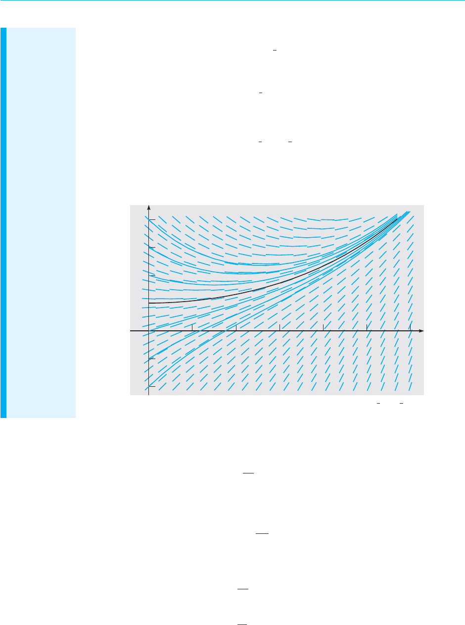
August 7, 2012 21:03 c02 Sheet number 4 Page number 34 cyan black
34 Chapter 2. First Order Differential Equations
By integrating both sides of Eq. (16), we obtain
e
t/2
y =
3
5
e
5t/6
+ c, (17)
where c is an arbitrary constant. Finally, on solving Eq. (17) for y,we have the general solution
of Eq. (9), namely,
y =
3
5
e
t/3
+ ce
−t/2
. (18)
To find the solution passing through the point (0,1), we set t = 0 and y = 1 in Eq. (18),
obtaining 1 = (3/5) + c. Thus c = 2 /5, and the desired solution is
y =
3
5
e
t/3
+
2
5
e
−t/2
. (19)
Figure 2.1.1 includes the graphs of Eq. (18) for several values of c with a direction field in
the background. The solution satisfying y(0) = 1 is shown by the black curve.
–2
–1
1
2
3
4
y
123456
t
FIGURE 2.1.1 Direction field and integral curves of y
′
+
1
2
y =
1
2
e
t/3
;
the black curve passes through the point (0, 1).
Let us now extend the method of integrating factors to equations of the form
dy
dt
+ ay = g(t), (20)
where a is a given constant and g(t) is a given function. Proceeding as in Example 2,
we find that the integrating factor µ(t) must satisfy
d µ
dt
= aµ, (21)
rather than Eq. (12). Thus the integrating factor is µ(t) = e
at
. Multiplying Eq. (20)
by µ(t), we obtain
e
at
dy
dt
+ ae
at
y = e
at
g(t),
or
d
dt
(e
at
y) = e
at
g(t). (22)

August 7, 2012 21:03 c02 Sheet number 5 Page number 35 cyan black
2.1 Linear Equations; Method of Integrating Factors 35
By integrating both sides of Eq. (22), we find that
e
at
y =
"
e
at
g(t) dt + c, (23)
where c is an arbitrary constant. For many simple functions g(t), we can evaluate the
integral in Eq. (23) and express the solution y in terms of elementary functions, as
in Example 2. However, for more complicated functions g(t), it is necessary to leave
the solution in integral form. In this case
y = e
−at
"
t
t
0
e
as
g(s) ds + ce
−at
. (24)
Note that in Eq. (24) we have used s to denote the integration variable to distinguish
it from the independent variable t, and we have chosen some convenient value t
0
as
the lower limit of integration.
EXAMPLE
3
Find the general solution of the differential equation
dy
dt
− 2y = 4 − t (25)
and plot the graphs of several solutions. Discuss the behavior of solutions as t →∞.
Equation (25) is of the form (20) with a =−2; therefore, the integrating factor is
µ(t) = e
−2t
. Multiplying the differential equation (25) by µ(t), we obtain
e
−2t
dy
dt
− 2e
−2t
y = 4e
−2t
− te
−2t
,
or
d
dt
(e
−2t
y) = 4e
−2t
− te
−2t
. (26)
Then, by integrating both sides of this equation, we have
e
−2t
y =−2e
−2t
+
1
2
te
−2t
+
1
4
e
−2t
+ c,
where we have used integration by parts on the last term in Eq. (26). Thus the general solution
of Eq. (25) is
y =−
7
4
+
1
2
t + ce
2t
. (27)
A direction field and graphs of the solution (27) for several values of c are shown in Figure
2.1.2. The behavior of the solution for large values of t is determined by the term ce
2t
. If c ̸= 0,
then the solution grows exponentially large in magnitude, with the same sign as c itself. Thus
the solutions diverge as t becomes large. The boundary between solutions that ultimately grow
positively and those that ultimately grow negatively occurs when c = 0. If we substitute c = 0
into Eq. (27) and then set t = 0, we find that y =−7/4 is the separation point on the y-axis.
Note that for this initial value, the solution is y =−
7
4
+
1
2
t; it grows positively, but linearly
rather than exponentially.

August 7, 2012 21:03 c02 Sheet number 6 Page number 36 cyan black
36 Chapter 2. First Order Differential Equations
y
0.5 1 1.5 2
t
–4
–3
–2
–1
FIGURE 2.1.2 Direction field and integral curves of y
′
− 2y = 4 − t.
Now we return to the general first order linear equation (3)
dy
dt
+ p(t)y = g(t),
where p and g are given functions. To determine an appropriate integrating factor,
we multiply Eq. (3) by an as yet undetermined function µ(t), obtaining
µ(t)
dy
dt
+ p(t)µ(t)y = µ(t)g(t). (28)
Following the same line of development as in Example 2, we see that the left side
of Eq. (28) is the derivative of the product µ(t)y, provided that µ(t) satisfies the
equation
d µ(t)
dt
= p(t)µ(t). (29)
If we assume temporarily that µ(t) is positive, then we have
d µ(t)/dt
µ(t)
= p(t),
and consequently
ln µ(t) =
"
p(t) dt + k.
By choosing the arbitrary constant k to be zero, we obtain the simplest possible
function for µ, namely,
µ(t) = exp
"
p(t) dt. (30)
Note that µ(t) is positive for all t, as we assumed. Returning to Eq. (28), we have
d
dt
[µ(t)y]=µ(t)g(t). (31)

August 7, 2012 21:03 c02 Sheet number 7 Page number 37 cyan black
2.1 Linear Equations; Method of Integrating Factors 37
Hence
µ(t)y =
"
µ(t)g(t) dt + c, (32)
where c is an arbitrary constant. Sometimes the integral in Eq.(32) can be evaluated
in terms of elementary functions. However, in general this is not possible, so the
general solution of Eq. (3) is
y =
1
µ(t)
%
"
t
t
0
µ(s)g (s ) ds + c
&
, (33)
where again t
0
is some convenient lower limit of integration. Observe that Eq. (33)
involves two integrations,one to obtain µ(t) from Eq. (30) and the other to determine
y from Eq. (33).
EXAMPLE
4
Solve the initial value problem
ty
′
+ 2y = 4t
2
, (34)
y(1) = 2. (35)
In order to determine p(t) and g(t) correctly, we must first rewrite Eq. (34) in the standard
form (3). Thus we have
y
′
+ (2/t)y = 4t, (36)
so p(t) = 2/t and g (t) = 4t. To solve Eq. (36), we first compute the integrating factor µ(t):
µ(t) = exp
"
2
t
dt = e
2 ln|t|
= t
2
.
On multiplying Eq. (36) by µ(t) = t
2
, we obtain
t
2
y
′
+ 2ty = (t
2
y)
′
= 4t
3
,
and therefore
t
2
y = t
4
+ c,
where c is an arbitrary constant. It follows that
y = t
2
+
c
t
2
(37)
is the general solution of Eq. (34). Integral curves of Eq. (34) for several values of c are shown
in Figure 2.1.3. To satisfy the initial condition (35), it is necessary to choose c = 1; thus
y = t
2
+
1
t
2
, t > 0 (38)
is the solution of the initial value problem (34), (35).This solution is shown by the black curve
in Figure 2.1.3. Note that it becomes unbounded and is asymptotic to the positive y-axis as
t → 0 from the right. This is the effect of the infinite discontinuity in the coefficient p(t) at
the origin. The function y = t
2
+ (1/t
2
) for t < 0 is not part of the solution of this initial value
problem.
This is the first example in which the solution fails to exist for some values of t. Again, this
is due to the infinite discontinuity in p(t) at t = 0, which restricts the solution to the interval
0 < t < ∞.
Looking again at Figure 2.1.3,we see that some solutions (those for which c > 0) are asymp-
totic to the positive y-axis as t → 0 from the right, while other solutions (for which c < 0)

August 7, 2012 21:03 c02 Sheet number 8 Page number 38 cyan black
38 Chapter 2. First Order Differential Equations
are asymptotic to the negative y-axis. The solution for which c = 0, namely, y = t
2
, remains
bounded and differentiable even at t = 0. If we generalize the initial condition (35) to
y(1) = y
0
, (39)
then c = y
0
− 1 and the solution (38) becomes
y = t
2
+
y
0
− 1
t
2
, t > 0 if y
0
̸= 1. (40)
As in Example 3, this is another instance where there is a critical initial value, namely, y
0
= 1,
that separates solutions that behave in one way from others that behave quite differently.
y
t
3
2
1
–1
11–
(1,
2)
FIGURE 2.1.3 Integral curves of the differential equation ty
′
+ 2y = 4t
2
;
the black curve passes through the point (1, 2).
EXAMPLE
5
Solve the initial value problem
2y
′
+ ty = 2, (41)
y(0) = 1. (42)
To convert the differential equation (41) to the standard form (3), we must divide by 2,
obtaining
y
′
+ (t/2)y = 1. (43)
Thus p(t) = t/2, and the integrating factor is µ(t) = exp(t
2
/4). Then multiply Eq. (43) by µ(t),
so that
e
t
2
/4
y
′
+
t
2
e
t
2
/4
y = e
t
2
/4
. (44)
The left side of Eq. (44) is the derivative of e
t
2
/4
y, so by integrating both sides of Eq. (44), we
obtain
e
t
2
/4
y =
"
e
t
2
/4
dt + c. (45)

August 7, 2012 21:03 c02 Sheet number 9 Page number 39 cyan black
2.1 Linear Equations; Method of Integrating Factors 39
The integral on the right side of Eq. (45) cannot be evaluated in terms of the usual elementary
functions, so we leave the integral unevaluated. However, by choosing the lower limit of
integration as the initial point t = 0, we can replace Eq. (45) by
e
t
2
/4
y =
"
t
0
e
s
2
/4
ds + c, (46)
where c is an arbitrary constant. It then follows that the general solution y of Eq. (41) is
given by
y = e
−t
2
/4
"
t
0
e
s
2
/4
ds + ce
−t
2
/4
. (47)
The initial condition (42) requires that c = 1.
The main purpose of this example is to illustrate that sometimes the solution must be left in
terms of an integral.This is usually at most a slight inconvenience,rather than a serious obstacle.
For a given value of t, the integral in Eq. (47) is a definite integral and can be approximated to
any desired degree of accuracy by using readily available numerical integrators. By repeating
this process for many values of t and plotting the results, you can obtain a graph of a solution.
Alternatively, you can use a numerical approximation method, such as those discussed in
Chapter 8, that proceed directly from the differential equation and need no expression for the
solution. Software packages such as Maple and Mathematica readily execute such procedures
and produce graphs of solutions of differential equations.
Figure 2.1.4 displays graphs of the solution (47) for several values of c. From the figure it
may be plausible to conjecture that all solutions approach a limit as t →∞. The limit can be
found analytically (see Problem 32).
–3
–2
–1
1
2
3
y
1234
5
6
t
FIGURE 2.1.4 Integral curves of 2y
′
+ ty = 2.
PROBLEMS In each of Problems 1 through 12:
(a) Draw a direction field for the given differential equation.
(b) Based on an inspection of the direction field, describe how solutions behave for large t.
(c) Find the general solution of the given differential equation, and use it to determine how
solutions behave as t →∞.

August 7, 2012 21:03 c02 Sheet number 10 Page number 40 cyan black
40 Chapter 2. First Order Differential Equations
1. y
′
+ 3y = t + e
−2t
2. y
′
− 2y = t
2
e
2t
3. y
′
+ y = te
−t
+ 14.y
′
+ (1/t)y = 3 cos 2 t, t > 0
5.
y
′
− 2y = 3e
t
6. ty
′
+ 2y = sin t, t > 0
7.
y
′
+ 2ty = 2te
−t
2
8. (1 + t
2
)y
′
+ 4ty = (1 + t
2
)
−2
9. 2y
′
+ y = 3t 10. ty
′
− y = t
2
e
−t
, t > 0
11.
y
′
+ y = 5 sin 2t 12. 2y
′
+ y = 3t
2
In each of Problems 13 through 20, find the solution of the given initial value problem.
13. y
′
− y = 2te
2t
, y(0) = 1
14. y
′
+ 2y = te
−2t
, y(1) = 0
15. ty
′
+ 2y = t
2
− t + 1, y(1) =
1
2
, t > 0
16. y
′
+ (2/t)y = (cos t)/t
2
, y(π) = 0, t > 0
17. y
′
− 2y = e
2t
, y(0) = 2
18. ty
′
+ 2y = sin t, y(π/2) = 1, t > 0
19. t
3
y
′
+ 4t
2
y = e
−t
, y(−1) = 0, t < 0
20. ty
′
+ (t + 1)y = t, y(ln 2) = 1, t > 0
In each of Problems 21 through 23:
(a) Draw a direction field for the given differential equation. How do solutions appear to
behave as t becomes large? Does the behavior depend on the choice of the initial value a?
Let a
0
be the value of a for which the transition from one type of behavior to another occurs.
Estimate the value of a
0
.
(b) Solve the initial value problem and find the critical value a
0
exactly.
(c) Describe the behavior of the solution corresponding to the initial value a
0
.
21.
y
′
−
1
2
y = 2 cos t, y(0) = a
22.
2y
′
− y = e
t/3
, y(0) = a
23.
3y
′
− 2y = e
−πt/2
, y(0) = a
In each of Problems 24 through 26:
(a) Draw a direction field for the given differential equation. How do solutions appear to
behave as t → 0? Does the behavior depend on the choice of the initial value a? Let a
0
be the
value of a for which the transition from one type of behavior to another occurs. Estimate the
value of a
0
.
(b) Solve the initial value problem and find the critical value a
0
exactly.
(c) Describe the behavior of the solution corresponding to the initial value a
0
.
24.
ty
′
+ (t + 1)y = 2te
−t
, y(1) = a, t > 0
25.
ty
′
+ 2y = (sin t)/t, y(−π/2) = a, t < 0
26.
(sin t)y
′
+ (cos t)y = e
t
, y(1) = a,0< t <π
27.
Consider the initial value problem
y
′
+
1
2
y = 2 cos t, y(0) =−1.
Find the coordinates of the first local maximum point of the solution for t > 0.
28.
Consider the initial value problem
y
′
+
2
3
y = 1 −
1
2
t, y(0) = y
0
.
Find the value of y
0
for which the solution touches, but does not cross, the t-axis.

August 7, 2012 21:03 c02 Sheet number 11 Page number 41 cyan black
2.1 Linear Equations; Method of Integrating Factors 41
29. Consider the initial value problem
y
′
+
1
4
y = 3 + 2 cos 2t, y(0) = 0.
(a) Find the solution of this initial value problem and describe its behavior for large t.
(b) Determine the value of t for which the solution first intersects the line y = 12.
30. Find the value of y
0
for which the solution of the initial value problem
y
′
− y = 1 + 3 sin t, y(0) = y
0
remains finite as t →∞.
31. Consider the initial value problem
y
′
−
3
2
y = 3t + 2e
t
, y(0) = y
0
.
Find the value of y
0
that separates solutions that grow positively as t →∞from those
that grow negatively. How does the solution that corresponds to this critical value of y
0
behave as t →∞?
32. Show that all solutions of 2y
′
+ ty = 2 [Eq. (41) of the text] approach a limit as t →∞,
and find the limiting value.
Hint: Consider the general solution, Eq. (47), and use L’Hôpital’s rule on the first term.
33. Show that if a and λ are positive constants, and b is any real number, then every solution
of the equation
y
′
+ ay = be
−λt
has the property that y → 0 as t →∞.
Hint: Consider the cases a = λ and a ̸= λ separately.
In each of Problems 34 through 37, construct a first order linear differential equation whose
solutions have the required behavior as t →∞. Then solve your equation and confirm that
the solutions do indeed have the specified property.
34. All solutions have the limit 3 as t →∞.
35. All solutions are asymptotic to the line y = 3 − t as t →∞.
36. All solutions are asymptotic to the line y = 2t − 5 as t →∞.
37. All solutions approach the curve y = 4 − t
2
as t →∞.
38. Variation of Parameters. Consider the following method of solving the general linear
equation of first order:
y
′
+ p(t)y = g(t). (i)
(a) If g(t) = 0 for all t, show that the solution is
y = A exp
%
−
"
p(t) dt
&
, (ii)
where A is a constant.
(b) If g(t) is not everywhere zero, assume that the solution of Eq. (i) is of the form
y = A(t) exp
%
−
"
p(t) dt
&
, (iii)

August 7, 2012 21:03 c02 Sheet number 12 Page number 42 cyan black
42 Chapter 2. First Order Differential Equations
where A is now a function of t. By substituting for y in the given differential equation,
show that A(t) must satisfy the condition
A
′
(t) = g(t) exp
%
"
p(t) dt
&
. (iv)
(c) Find A(t) from Eq. (iv). Then substitute for A(t) in Eq. (iii) and determine y. Verify
that the solution obtained in this manner agrees with that of Eq. (33) in the text. This
technique is known as the method of variation of parameters; it is discussed in detail in
Section 3.6 in connection with second order linear equations.
In each of Problems 39 through 42,use the method of Problem 38 to solve the given differential
equation.
39. y
′
− 2y = t
2
e
2t
40. y
′
+ (1/t)y = 3 cos 2 t, t > 0
41. ty
′
+ 2y = sin t, t > 0 42. 2y
′
+ y = 3t
2
2.2 Separable Equations
In Section 1.2 we used a process of direct integration to solve first order linear
equations of the form
dy
dt
= ay + b, (1)
where a and b are constants. We will now show that this process is actually applicable
to a much larger class of equations.
We will use x, rather than t, to denote the independent variable in this section for
two reasons. In the first place,different letters are frequently used for the variables in
a differential equation, and you should not become too accustomed to using a single
pair. In particular, x often occurs as the independent variable. Further, we want to
reserve t for another purpose later in the section.
The general first order equation is
dy
dx
= f (x, y). (2)
Linear equations were considered in the preceding section,but if Eq. (2) is nonlinear,
then there is no universally applicable method for solving the equation. Here, we
consider a subclass of first order equations that can be solved by direct integration.
To identify this class of equations, we first rewrite Eq. (2) in the form
M(x, y) + N(x, y)
dy
dx
= 0. (3)
It is always possible to do this by setting M(x, y) =−f (x, y) and N(x, y) = 1, but there
may be other ways as well. If it happens that M is a function of x only and N is a
function of y only, then Eq. (3) becomes
M(x) + N(y)
dy
dx
= 0. (4)

August 7, 2012 21:03 c02 Sheet number 13 Page number 43 cyan black
2.2 Separable Equations 43
Such an equation is said to be separable, because if it is written in the differential
form
M(x) dx + N(y) dy = 0, (5)
then, if you wish, terms involving each variable may be placed on opposite sides
of the equation. The differential form (5) is also more symmetric and tends to
suppress the distinction between independent and dependent variables.
A separable equation can be solved by integrating the functions M and N.
We illustrate the process by an example and then discuss it in general for Eq. (4).
EXAMPLE
1
Show that the equation
dy
dx
=
x
2
1 − y
2
(6)
is separable, and then find an equation for its integral curves.
If we write Eq. (6) as
−x
2
+ (1 − y
2
)
dy
dx
= 0, (7)
then it has the form (4) and is therefore separable. Recall from calculus that if y is a function
of x, then by the chain rule,
d
dx
f (y) =
d
dy
f (y)
dy
dx
= f
′
(y)
dy
dx
.
For example, if f (y) = y − y
3
/3, then
d
dx
(y − y
3
/3) = (1 − y
2
)
dy
dx
.
Thus the second term in Eq. (7) is the derivative with respect to x of y − y
3
/3, and the first
term is the derivative of −x
3
/3. Thus Eq. (7) can be written as
d
dx
'
−
x
3
3
(
+
d
dx
'
y −
y
3
3
(
= 0,
or
d
dx
'
−
x
3
3
+ y −
y
3
3
(
= 0.
Therefore, by integrating, we obtain
−x
3
+ 3y − y
3
= c, (8)
where c is an arbitrary constant. Equation (8) is an equation for the integral curves of Eq. (6).
A direction field and several integral curves are shown in Figure 2.2.1. Any differentiable
function y = φ(x) that satisfies Eq. (8) is a solution of Eq. (6). An equation of the integral
curve passing through a particular point (x
0
, y
0
) can be found by substituting x
0
and y
0
for x
and y, respectively, in Eq. (8) and determining the corresponding value of c.

August 7, 2012 21:03 c02 Sheet number 14 Page number 44 cyan black
44 Chapter 2. First Order Differential Equations
4
2
422–4–
–2
–4
y
x
FIGURE 2.2.1 Direction field and integral curves of y
′
= x
2
/(1 − y
2
).
Essentially the same procedure can be followed for any separable equation.
Returning to Eq. (4), let H
1
and H
2
be any antiderivatives of M and N, respectively.
Thus
H
′
1
(x) = M(x), H
′
2
(y) = N(y), (9)
and Eq. (4) becomes
H
′
1
(x) + H
′
2
(y)
dy
dx
= 0. (10)
If y is regarded as a function of x, then according to the chain rule,
H
′
2
(y)
dy
dx
=
d
dy
H
2
(y)
dy
dx
=
d
dx
H
2
(y). (11)
Consequently, we can write Eq. (10) as
d
dx
[H
1
(x) + H
2
(y)]=0. (12)
By integrating Eq. (12), we obtain
H
1
(x) + H
2
(y) = c, (13)
where c is an arbitrary constant. Any differentiable function y = φ(x) that satisfies
Eq. (13) is a solution of Eq. (4); in other words, Eq. (13) defines the solution implic-
itly rather than explicitly. In practice, Eq. (13) is usually obtained from Eq. (5) by
integrating the first term with respect to x and the second term with respect to y.The
justification for this is the argument that we have just given.
The differential equation (4), together with an initial condition
y(x
0
) = y
0
, (14)

August 7, 2012 21:03 c02 Sheet number 15 Page number 45 cyan black
2.2 Separable Equations 45
forms an initial value problem.To solve this initial value problem,we must determine
the appropriate value for the constant c in Eq. (13). We do this by setting x = x
0
and
y = y
0
in Eq. (13) with the result that
c = H
1
(x
0
) + H
2
(y
0
). (15)
Substituting this value of c in Eq. (13) and noting that
H
1
(x) − H
1
(x
0
) =
"
x
x
0
M(s) ds, H
2
(y) − H
2
(y
0
) =
"
y
y
0
N(s) ds,
we obtain
"
x
x
0
M(s) ds +
"
y
y
0
N(s) ds = 0. (16)
Equation (16) is an implicit representation of the solution of the differential equation
(4) that also satisfies the initial condition (14). Bear in mind that to determine an
explicit formula for the solution, you need to solve Eq. (16) for y as a function of x.
Unfortunately, it is often impossible to do this analytically; in such cases you can
resort to numerical methods to find approximate values of y for given values of x.
EXAMPLE
2
Solve the initial value problem
dy
dx
=
3x
2
+ 4x + 2
2(y − 1)
, y(0) =−1, (17)
and determine the interval in which the solution exists.
The differential equation can be written as
2(y − 1) dy = (3x
2
+ 4x + 2) dx.
Integrating the left side with respect to y and the right side with respect to x gives
y
2
− 2y = x
3
+ 2x
2
+ 2x + c, (18)
where c is an arbitrary constant. To determine the solution satisfying the prescribed initial
condition, we substitute x = 0 and y =−1 in Eq. (18), obtaining c = 3. Hence the solution of
the initial value problem is given implicitly by
y
2
− 2y = x
3
+ 2x
2
+ 2x + 3. (19)
To obtain the solution explicitly, we must solve Eq. (19) for y in terms of x. That is a simple
matter in this case, since Eq. (19) is quadratic in y, and we obtain
y = 1 ±
!
x
3
+ 2x
2
+ 2x + 4. (20)
Equation (20) gives two solutions of the differential equation, only one of which, however,
satisfies the given initial condition. This is the solution corresponding to the minus sign in
Eq. (20), so we finally obtain
y = φ(x) = 1 −
!
x
3
+ 2x
2
+ 2x + 4 (21)
as the solution of the initial value problem (17). Note that if we choose the plus sign by mistake
in Eq. (20),then we obtain the solution of the same differential equation that satisfies the initial
condition y(0) = 3. Finally,to determine the interval in which the solution (21) is valid,we must
find the interval in which the quantity under the radical is positive. The only real zero of this
expression is x =−2, so the desired interval is x > −2. Some integral curves of the differential

August 7, 2012 21:03 c02 Sheet number 16 Page number 46 cyan black
46 Chapter 2. First Order Differential Equations
equation are shown in Figure 2.2.2. The black curve passes through the point (0, −1) and thus
is the solution of the initial value problem (17). Observe that the boundary of the interval
of validity of the solution (21) is determined by the point (−2, 1) at which the tangent line is
vertical.
y
x
11––2
(–2, 1)
2
–2
–1
1
2
3
(0, –1)
FIGURE 2.2.2 Integral curves of y
′
= (3x
2
+ 4x + 2)/2(y − 1); the
solution satisfying y(0) =−1 is shown in black and is valid for x > −2.
EXAMPLE
3
Solve the equation
dy
dx
=
4x − x
3
4 + y
3
(22)
and draw graphs of several integral curves. Also find the solution passing through the point
(0, 1) and determine its interval of validity.
Rewriting Eq. (22) as
(4 + y
3
) dy = (4x − x
3
) dx,
integrating each side, multiplying by 4, and rearranging the terms, we obtain
y
4
+ 16y + x
4
− 8x
2
= c, (23)
where c is an arbitrary constant. Any differentiable function y = φ(x) that satisfies Eq. (23)
is a solution of the differential equation (22). Graphs of Eq. (23) for several values of c are
shown in Figure 2.2.3.
To find the particular solution passing through (0, 1),we set x = 0 and y = 1 in Eq. (23) with
the result that c = 17. Thus the solution in question is given implicitly by
y
4
+ 16y + x
4
− 8x
2
= 17. (24)
It is shown by the black curve in Figure 2.2.3. The interval of validity of this solution extends
on either side of the initial point as long as the function remains differentiable. From the
figure we see that the interval ends when we reach points where the tangent line is verti-
cal. It follows from the differential equation (22) that these are points where 4 + y
3
= 0, or

August 7, 2012 21:03 c02 Sheet number 17 Page number 47 cyan black
2.2 Separable Equations 47
–3
–2
–1
1
2
y
–3 –2 –1 123
x
)4785.1– ,8843.3()4785.1– ,8843.3–(
FIGURE 2.2.3 Integral curves of y
′
= (4x − x
3
)/(4 + y
3
).
The solution passing through (0, 1) is shown by the black curve.
y = (−4)
1/3
∼
=
−1.5874. From Eq. (24) the corresponding values of x are x
∼
=
±3.3488. These
points are marked on the graph in Figure 2.2.3.
Note 1: Sometimes an equation of the form (2)
dy
dx
= f (x, y)
has a constant solution y = y
0
. Such a solution is usually easy to find because if
f (x, y
0
) = 0 for some value y
0
and for all x, then the constant function y = y
0
is a
solution of the differential equation (2). For example, the equation
dy
dx
=
(y − 3) cos x
1 + 2y
2
(25)
has the constant solution y = 3. Other solutions of this equation can be found by
separating the variables and integrating.
Note 2: The investigation of a first order nonlinear equation can sometimes be
facilitated by regarding both x and y as functions of a third variable t. Then
dy
dx
=
dy/dt
dx/dt
. (26)
If the differential equation is
dy
dx
=
F(x, y)
G(x, y)
, (27)

August 7, 2012 21:03 c02 Sheet number 18 Page number 48 cyan black
48 Chapter 2. First Order Differential Equations
then, by comparing numerators and denominators in Eqs. (26) and (27), we obtain
the system
dx/dt = G(x, y), dy/dt = F(x, y). (28)
At first sight it may seem unlikely that a problem will be simplified by replacing a
single equation by a pair of equations, but in fact, the system (28) may well be more
amenable to investigation than the single equation (27). Chapter 9 is devoted to
nonlinear systems of the form (28).
Note 3: In Example 2 it was not difficult to solve explicitly for y as a function
of x. However, this situation is exceptional, and often it will be better to leave the
solution in implicit form, as in Examples 1 and 3. Thus, in the problems below and
in other sections where nonlinear equations appear, the words “solve the following
differential equation” mean to find the solution explicitly if it is convenient to do so,
but otherwise to find an equation defining the solution implicitly.
PROBLEMS In each of Problems 1 through 8, solve the given differential equation.
1. y
′
= x
2
/y 2. y
′
= x
2
/y(1 + x
3
)
3. y
′
+ y
2
sin x = 04.y
′
= (3x
2
− 1)/(3 + 2y)
5. y
′
= (cos
2
x)(cos
2
2y) 6. xy
′
= (1 − y
2
)
1/2
7.
dy
dx
=
x − e
−x
y + e
y
8.
dy
dx
=
x
2
1 + y
2
In each of Problems 9 through 20:
(a) Find the solution of the given initial value problem in explicit form.
(b) Plot the graph of the solution.
(c) Determine (at least approximately) the interval in which the solution is defined.
9.
y
′
= (1 − 2x)y
2
, y(0) =−1/6 10. y
′
= (1 − 2x)/y, y(1) =−2
11.
xdx+ ye
−x
dy = 0, y(0) = 1 12. dr/dθ = r
2
/θ, r(1) = 2
13.
y
′
= 2x/(y + x
2
y), y(0) =−2 14. y
′
= xy
3
(1 + x
2
)
−1/2
, y(0) = 1
15.
y
′
= 2x/(1 + 2y), y(2) = 0 16. y
′
= x(x
2
+ 1)/4y
3
, y(0) =−1/
√
2
17.
y
′
= (3x
2
− e
x
)/(2y − 5), y(0) = 1
18.
y
′
= (e
−x
− e
x
)/(3 + 4y), y(0) = 1
19.
sin 2xdx+cos 3ydy = 0, y(π/2) = π/3
20.
y
2
(1 − x
2
)
1/2
dy = arcsin xdx, y(0) = 1
Some of the results requested in Problems 21 through 28 can be obtained either by solving
the given equations analytically or by plotting numerically generated approximations to the
solutions. Try to form an opinion about the advantages and disadvantages of each approach.
21.
Solve the initial value problem
y
′
= (1 + 3x
2
)/(3y
2
− 6y), y(0) = 1
and determine the interval in which the solution is valid.
Hint: To find the interval of definition, look for points where the integral curve has a
vertical tangent.

August 7, 2012 21:03 c02 Sheet number 19 Page number 49 cyan black
2.2 Separable Equations 49
22. Solve the initial value problem
y
′
= 3x
2
/(3y
2
− 4), y(1) = 0
and determine the interval in which the solution is valid.
Hint: To find the interval of definition, look for points where the integral curve has a
vertical tangent.
23.
Solve the initial value problem
y
′
= 2y
2
+ xy
2
, y(0) = 1
and determine where the solution attains its minimum value.
24.
Solve the initial value problem
y
′
= (2 − e
x
)/(3 + 2y), y(0) = 0
and determine where the solution attains its maximum value.
25.
Solve the initial value problem
y
′
= 2 cos 2x/(3 + 2y), y(0) =−1
and determine where the solution attains its maximum value.
26.
Solve the initial value problem
y
′
= 2(1 + x)(1 + y
2
), y(0) = 0
and determine where the solution attains its minimum value.
27.
Consider the initial value problem
y
′
= ty(4 − y)/3, y(0) = y
0
.
(a) Determine how the behavior of the solution as t increases depends on the initial
value y
0
.
(b) Suppose that y
0
= 0.5. Findthe time T at which the solution first reaches the value 3.98.
28.
Consider the initial value problem
y
′
= ty(4 − y)/(1 + t), y(0) = y
0
> 0.
(a) Determine how the solution behaves as t →∞.
(b) If y
0
= 2, find the time T at which the solution first reaches the value 3.99.
(c) Findthe range of initial values for which the solution lies in the interval 3.99 < y < 4.01
by the time t = 2.
29. Solve the equation
dy
dx
=
ay + b
cy + d
,
where a, b, c, and d are constants.
Homogeneous Equations. If the right side of the equation dy/dx = f (x, y) can
be expressed as a function of the ratio y/x only, then the equation is said to be

August 7, 2012 21:03 c02 Sheet number 20 Page number 50 cyan black
50 Chapter 2. First Order Differential Equations
homogeneous.
1
Such equations can always be transformed into separable equations
by a change of the dependent variable. Problem 30 illustrates how to solve first order
homogeneous equations.
30.
Consider the equation
dy
dx
=
y − 4x
x − y
. (i)
(a) Show that Eq. (i) can be rewritten as
dy
dx
=
(y/x) − 4
1 − (y/x)
; (ii)
thus Eq. (i) is homogeneous.
(b) Introduce a new dependent variable v so that v = y/x, or y = xv(x). Express dy/dx in
terms of x, v, and dv/dx.
(c) Replace y and dy/dx in Eq. (ii) by the expressions from part (b) that involve v and
dv/dx. Show that the resulting differential equation is
v + x
dv
dx
=
v − 4
1 − v
,
or
x
dv
dx
=
v
2
− 4
1 − v
. (iii)
Observe that Eq. (iii) is separable.
(d) Solve Eq. (iii), obtaining v implicitly in terms of x.
(e) Find the solution of Eq. (i) by replacing v by y/x in the solution in part (d).
(f) Draw a direction field and some integral curves for Eq. (i). Recall that the right side
of Eq. (i) actually depends only on the ratio y/x. This means that integral curves have
the same slope at all points on any given straight line through the origin, although the
slope changes from one line to another. Therefore, the direction field and the integral
curves are symmetric with respect to the origin. Is this symmetry property evident from
your plot?
The method outlined in Problem 30 can be used for any homogeneous equation. That
is, the substitution y = xv(x) transforms a homogeneous equation into a separable
equation. The latter equation can be solved by direct integration, and then replacing v
by y/x gives the solution to the original equation. In each of Problems 31 through 38:
(a) Show that the given equation is homogeneous.
(b) Solve the differential equation.
(c) Draw a direction field and some integral curves. Are they symmetric with respect to
the origin?
31.
dy
dx
=
x
2
+ xy + y
2
x
2
32.
dy
dx
=
x
2
+ 3y
2
2xy
33.
dy
dx
=
4y − 3x
2x − y
34.
dy
dx
=−
4x + 3y
2x + y
1
The word “homogeneous” has different meanings in different mathematical contexts. The homogeneous
equations considered here have nothing to do with the homogeneous equations that will occur in Chapter 3
and elsewhere.

August 7, 2012 21:03 c02 Sheet number 21 Page number 51 cyan black
2.3 Modeling with First Order Equations 51
35.
dy
dx
=
x + 3y
x − y
36.
(x
2
+ 3xy + y
2
) dx − x
2
dy = 0
37.
dy
dx
=
x
2
− 3y
2
2xy
38.
dy
dx
=
3y
2
− x
2
2xy
2.3 Modeling with First Order Equations
Differential equations are of interest to nonmathematicians primarily because of the
possibility of using them to investigate a wide variety of problems in the physical,
biological, and social sciences. One reason for this is that mathematical models and
their solutions lead to equations relating the variables and parameters in the prob-
lem. These equations often enable you to make predictions about how the natural
process will behave in various circumstances. It is often easy to vary parameters in
the mathematical model over wide ranges, whereas this may be very time-consuming
or expensive, if not impossible, in an experimental setting. Nevertheless, mathemat-
ical modeling and experiment or observation are both critically important and have
somewhat complementary roles in scientific investigations. Mathematical models are
validated by comparison of their predictions with experimental results. On the other
hand, mathematical analyses may suggest the most promising directions to explore
experimentally, and they may indicate fairly precisely what experimental data will
be most helpful.
In Sections 1.1 and 1.2 we formulated and investigated a few simple mathemat-
ical models. We begin by recapitulating and expanding on some of the conclusions
reached in those sections. Regardless of the specific field of application, there are
three identifiable steps that are always present in the process of mathematical
modeling.
Construction of the Model. In this step you translate the physical situation into math-
ematical terms, often using the steps listed at the end of Section 1.1. Perhaps most
critical at this stage is to state clearly the physical principle(s) that are believed to
govern the process. For example, it has been observed that in some circumstances
heat passes from a warmer to a cooler body at a rate proportional to the temperature
difference,that objects move about in accordance with Newton’s laws of motion, and
that isolated insect populations grow at a rate proportional to the current population.
Each of these statements involves a rate of change (derivative) and consequently,
when expressed mathematically, leads to a differential equation. The differential
equation is a mathematical model of the process.
It is important to realize that the mathematical equations are almost always only
an approximate description of the actual process. For example, bodies moving at
speeds comparable to the speed of light are not governed by Newton’s laws, insect
populations do not grow indefinitely as stated because of eventual lack of food or
space, and heat transfer is affected by factors other than the temperature difference.
Thus you should always be aware of the limitations of the model so that you will use
it only when it is reasonable to believe that it is accurate.Alternatively, you can adopt
the point of view that the mathematical equations exactly describe the operation of

August 7, 2012 21:03 c02 Sheet number 22 Page number 52 cyan black
52 Chapter 2. First Order Differential Equations
a simplified physical model, which has been constructed (or conceived of) so as to
embody the most important features of the actual process. Sometimes, the process
of mathematical modeling involves the conceptual replacement of a discrete process
by a continuous one. For instance, the number of members in an insect population
changes by discrete amounts; however, if the population is large, it seems reasonable
to consider it as a continuous variable and even to speak of its derivative.
Analysis of the Model. Once the problem has been formulated mathematically, you are
often faced with the problem of solving one or more differential equations or, failing
that, of finding out as much as possible about the properties of the solution. It may
happen that this mathematical problem is quite difficult,and if so,further approxima-
tions may be indicated at this stage to make the problem mathematically tractable.
For example, a nonlinear equation may be approximated by a linear one, or a slowly
varying coefficient may be replaced by a constant. Naturally, any such approxima-
tions must also be examined from the physical point of view to make sure that the
simplified mathematical problem still reflects the essential features of the physical
process under investigation. At the same time, an intimate knowledge of the physics
of the problem may suggest reasonable mathematical approximations that will make
the mathematical problem more amenable to analysis. This interplay of understand-
ing of physical phenomena and knowledge of mathematical techniques and their
limitations is characteristic of applied mathematics at its best, and it is indispens-
able in successfully constructing useful mathematical models of intricate physical
processes.
Comparison with Experiment or Obser vation. Finally, having obtained the solution (or at
least some information about it), you must interpret this information in the con-
text in which the problem arose. In particular, you should always check that the
mathematical solution appears physically reasonable. If possible,calculate the values
of the solution at selected points and compare them with experimentally observed
values. Or ask whether the behavior of the solution after a long time is consistent
withobservations. Or examine thesolutions corresponding tocertain special values of
parameters in the problem. Of course,the fact that the mathematical solution appears
to be reasonable does not guarantee that it is correct. However, if the predictions of
the mathematical model are seriously inconsistent with observations of the physical
system it purports to describe, this suggests that errors have been made in solving
the mathematical problem, that the mathematical model itself needs refinement, or
that observations must be made with greater care.
The examples in this section are typical of applications in which first order differ-
ential equations arise.
EXAMPLE
1
Mixing
At time t = 0 a tank contains Q
0
lb of salt dissolved in 100 gal of water;see Figure 2.3.1.Assume
that water containing
1
4
lb of salt/gal is entering the tank at a rate of r gal/min and that the
well-stirred mixture is draining from the tank at the same rate. Set up the initial value problem
that describes this flow process. Find the amount of salt Q(t) in the tank at any time, and also
find the limiting amount Q
L
that is present after a very long time. If r = 3 and Q
0
= 2Q
L
, find
the time T after which the salt level is within 2% of Q
L
. Also find the flow rate that is required
if the value of T is not to exceed 45 min.
We assume that salt is neither created nor destroyed in the tank. Therefore, variations in
the amount of salt are due solely to the flows in and out of the tank. More precisely, the rate

August 7, 2012 21:03 c02 Sheet number 23 Page number 53 cyan black
2.3 Modeling with First Order Equations 53
of change of salt in the tank, dQ/dt, is equal to the rate at which salt is flowing in minus the
rate at which it is flowing out. In symbols,
dQ
dt
= rate in − rate out. (1)
The rate at which salt enters the tank is the concentration
1
4
lb/gal times the flow rate r gal/min,
or (r/4) lb/min. To find the rate at which salt leaves the tank, we need to multiply the concen-
tration of salt in the tank by the rate of outflow, r gal/min. Since the rates of flow in and out
are equal, the volume of water in the tank remains constant at 100 gal, and since the mixture
is “well-stirred,” the concentration throughout the tank is the same, namely, [Q(t)/100] lb/gal.
Therefore, the rate at which salt leaves the tank is [rQ(t)/100] lb/min. Thus the differential
equation governing this process is
dQ
dt
=
r
4
−
rQ
100
. (2)
The initial condition is
Q(0) = Q
0
. (3)
r gal/min, lb/gal
1
4
r gal/min
FIGURE 2.3.1 The water tank in Example 1.
Upon thinking about the problem physically,wemight anticipate that eventually the mixture
originally in the tank will be essentially replaced by the mixture flowing in,whoseconcentration
is
1
4
lb/gal. Consequently, we might expect that ultimately the amount of salt in the tank would
be very close to 25 lb. We can also find the limiting amount Q
L
= 25 by setting dQ/dt equal
to zero in Eq. (2) and solving the resulting algebraic equation for Q.
To solve the initial value problem (2), (3) analytically, note that Eq. (2) is both linear and
separable. Rewriting it in the standard form for a linear equation, we have
dQ
dt
+
rQ
100
=
r
4
. (4)
Thus the integrating factor is e
rt/100
and the general solution is
Q(t) = 25 + ce
−rt/100
, (5)
where c is an arbitrary constant.To satisfy the initial condition (3),wemust choose c = Q
0
− 25.
Therefore, the solution of the initial value problem (2), (3) is
Q(t) = 25 + (Q
0
− 25)e
−rt/100
, (6)
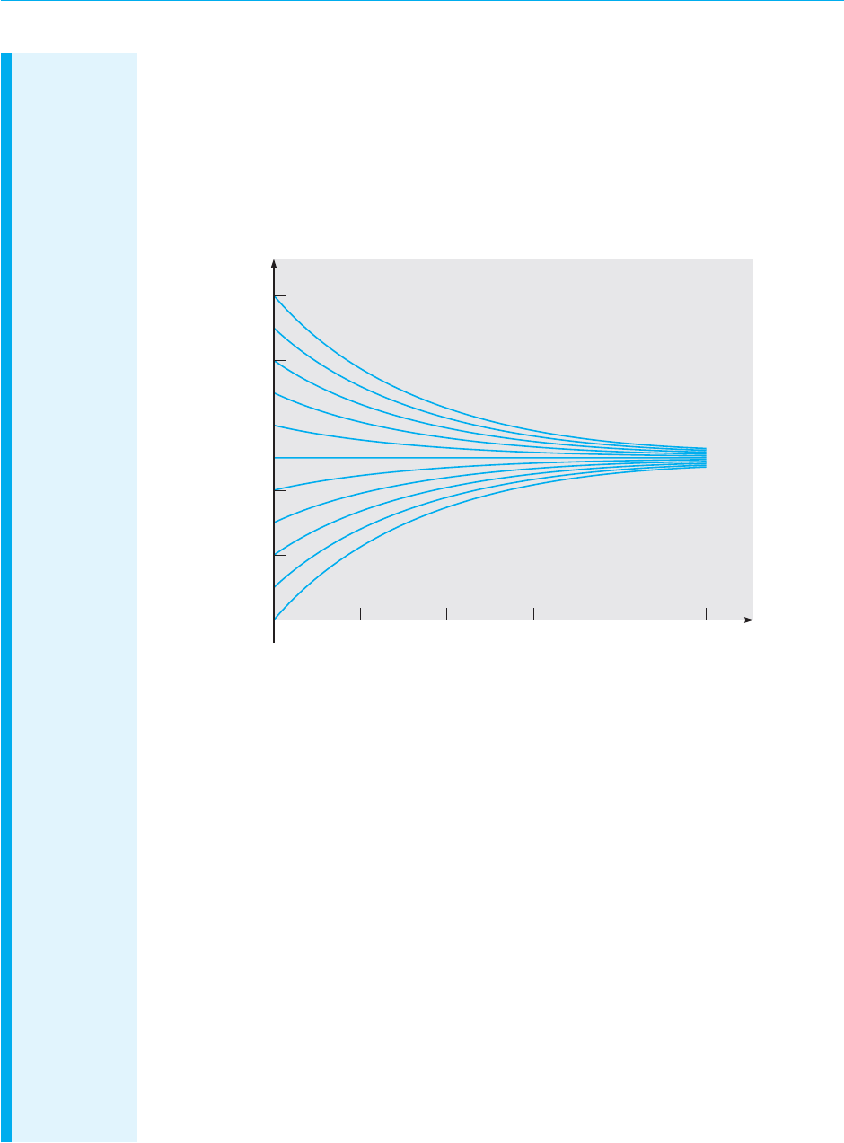
August 7, 2012 21:03 c02 Sheet number 24 Page number 54 cyan black
54 Chapter 2. First Order Differential Equations
or
Q(t) = 25(1 − e
−rt/100
) + Q
0
e
−rt/100
. (7)
From Eq. (6) or (7), you can see that Q(t) → 25 (lb) as t →∞, so the limiting value Q
L
is
25, confirming our physical intuition. Further, Q(t) approaches the limit more rapidly as r
increases. In interpreting the solution (7), note that the second term on the right side is the
portion of the original salt that remains at time t,while the first term gives the amount of salt in
the tank as a consequence of the flow processes. Plots of the solution for r = 3 and for several
values of Q
0
are shown in Figure 2.3.2.
50
40
30
20
10
20 40 60 80 100
Q
t
FIGURE 2.3.2 Solutions of the initial value problem (2), (3):
dQ/dt = (r/4 ) − rQ/100, Q(0) = Q
0
for r = 3 and several values of Q
0
.
Now suppose that r = 3 and Q
0
= 2Q
L
= 50; then Eq. (6) becomes
Q(t) = 25 + 25e
−0.03t
. (8)
Since 2% of 25 is 0.5, we wish to find the time T at which Q(t) has the value 25.5. Substituting
t = T and Q = 25.5 in Eq. (8) and solving for T, we obtain
T = (ln 50)/0.03
∼
=
130.4 (min). (9)
To determine r so that T = 45, return to Eq. (6), set t = 45, Q
0
= 50, Q(t) = 25.5, and solve
for r. The result is
r = (100/45) ln 50
∼
=
8.69 gal/min. (10)
Since this example is hypothetical, the validity of the model is not in question. If the flow
rates are as stated, and if the concentration of salt in the tank is uniform, then the differential
equation (1) is an accurate description of the flow process. Although this particular example
has no special significance,models of this kind are often used in problems involving a pollutant
in a lake, or a drug in an organ of the body, for example, rather than a tank of salt water. In
such cases the flow rates may not be easy to determine or may vary with time. Similarly, the
concentration may be far from uniform in some cases. Finally, the rates of inflow and outflow
may be different, which means that the variation of the amount of liquid in the problem must
also be taken into account.

August 7, 2012 21:03 c02 Sheet number 25 Page number 55 cyan black
2.3 Modeling with First Order Equations 55
EXAMPLE
2
Compound
Interest
Suppose that a sum of money is deposited in a bank or money fund that pays interest at an
annual rate r. The value S(t) of the investment at any time t depends on the frequency with
which interest is compounded as well as on the interest rate. Financial institutions have various
policies concerning compounding: some compound monthly, some weekly, some even daily.
If we assume that compounding takes place continuously, then we can set up an initial value
problem that describes the growth of the investment.
The rate of change of the value of the investment is dS/dt, and this quantity is equal to
the rate at which interest accrues, which is the interest rate r times the current value of the
investment S(t). Thus
dS/dt = rS (11)
is the differential equation that governs the process. Suppose that we also know the value of
the investment at some particular time, say,
S(0 ) = S
0
. (12)
Then the solution of the initial value problem (11), (12) gives the balance S(t) in the account
at any time t. This initial value problem is readily solved, since the differential equation (11)
is both linear and separable. Consequently, by solving Eqs. (11) and (12), we find that
S(t) = S
0
e
rt
. (13)
Thus a bank account with continuously compounding interest grows exponentially.
Let us now compare the results from this continuous model with the situation in which
compounding occurs at finite time intervals. If interest is compounded once a year, then after
t years
S(t) = S
0
(1 + r)
t
.
If interest is compounded twice a year, then at the end of 6 months the value of the investment
is S
0
[1 + (r/2)], and at the end of 1 year it is S
0
[1 + (r/2)]
2
. Thus, after t years we have
S(t) = S
0
)
1 +
r
2
*
2t
.
In general, if interest is compounded m times per year, then
S(t) = S
0
)
1 +
r
m
*
mt
. (14)
The relation between formulas (13) and (14) is clarified if we recall from calculus that
lim
m→∞
S
0
)
1 +
r
m
*
mt
= S
0
e
rt
.
The same model applies equally well to more general investments in which dividends and
perhaps capital gains can also accumulate, as well as interest. In recognition of this fact, we
will from now on refer to r as the rate of return.
Table 2.3.1 shows the effect of changing the frequency of compounding for a return rate
r of 8%. The second and third columns are calculated from Eq. (14) for quarterly and daily
compounding, respectively, and the fourth column is calculated from Eq. (13) for continuous
compounding. The results show that the frequency of compounding is not particularly impor-
tant in most cases. For example, during a 10-year period the difference between quarterly
and continuous compounding is $17.50 per $1000 invested, or less than $2/year. The differ-
ence would be somewhat greater for higher rates of return and less for lower rates. From the
first row in the table, we see that for the return rate r = 8%, the annual yield for quarterly
compounding is 8.24% and for daily or continuous compounding it is 8.33%.
Returning now to the case of continuous compounding, let us suppose that there may be
deposits or withdrawals in addition to the accrual of interest, dividends, or capital gains. If

August 7, 2012 21:03 c02 Sheet number 26 Page number 56 cyan black
56 Chapter 2. First Order Differential Equations
TABLE 2.3.1 Growth of Capital at a Return Rate r = 8%
for Several Modes of Compounding
S(t)/S(t
0
) from Eq.(14)
S(t)/S(t
0
)
Years m = 4 m = 365 from Eq. (13)
1 1.0824 1.0833 1.0833
2 1.1717 1.1735 1.1735
5 1.4859 1.4918 1.4918
10 2.2080 2.2253 2.2255
20 4.8754 4.9522 4.9530
30 10.7652 11.0203 11.0232
40 23.7699 24.5239 24.5325
we assume that the deposits or withdrawals take place at a constant rate k, then Eq. (11) is
replaced by
dS/dt = rS + k,
or, in standard form,
dS/dt − rS = k, (15)
where k is positive for deposits and negative for withdrawals.
Equation (15) is linear with the integrating factor e
−rt
, so its general solution is
S(t) = ce
rt
− (k/r),
where c is an arbitrary constant. To satisfy the initial condition (12), we must choose
c = S
0
+ (k/r). Thus the solution of the initial value problem (15), (12) is
S(t) = S
0
e
rt
+ (k/r)(e
rt
− 1). (16)
The first term in expression (16) is the part of S(t) that is due to the return accumulated on
the initial amount S
0
, and the second term is the part that is due to the deposit or withdrawal
rate k.
The advantage of stating the problem in this general way without specific values for S
0
, r,or
k lies in the generality of the resulting formula (16) for S(t). With this formula we can readily
compare the results of different investment programs or different rates of return.
For instance, suppose that one opens an individual retirement account (IRA) at age 25 and
makes annual investments of $2000 thereafter in a continuous manner. Assuming a rate of
return of 8%, what will be the balance in the IRA at age 65? We have S
0
= 0, r = 0.08, and
k = $2000, and we wish to determine S(40). From Eq. (16) we have
S(40 ) = (25,000)(e
3.2
− 1) = $588,313. (17)
It is interesting to note that the total amount invested is $80,000, so the remaining amount of
$508,313 results from the accumulated return on the investment. The balance after 40 years
is also fairly sensitive to the assumed rate. For instance, S(40) = $508,948 if r = 0.075 and
S(40 ) = $681,508 if r = 0.085.
Let us now examine the assumptions that have gone into the model. First,we have assumed
that the return is compounded continuously and that additional capital is invested continu-
ously. Neither of these is true in an actual financial situation. We have also assumed that the
return rate r is constant for the entire period involved, whereas in fact it is likely to fluctuate
considerably. Although we cannot reliably predict future rates, we can use expression (16) to

August 7, 2012 21:03 c02 Sheet number 27 Page number 57 cyan black
2.3 Modeling with First Order Equations 57
determine the approximate effect of different rate projections. It is also possible to consider
r and k in Eq. (15) to be functions of t rather than constants;in that case,of course,the solution
may be much more complicated than Eq. (16).
The initial value problem (15), (12) and the solution (16) can also be used to analyze a
number of other financial situations, including annuities, mortgages, and automobile loans.
EXAMPLE
3
Chemicals in
aPond
Consider a pond that initially contains 10 million gal of fresh water. Water containing an
undesirable chemical flows into the pond at the rate of 5 million gal/yr, and the mixture in
the pond flows out at the same rate. The concentration γ(t) of chemical in the incoming water
varies periodically with time according to the expression γ(t) = 2 + sin 2t g/gal. Construct a
mathematical model of this flow process and determine the amount of chemical in the pond
at any time. Plot the solution and describe in words the effect of the variation in the incoming
concentration.
Since the incoming and outgoing flows of water are the same, the amount of water in the
pond remains constant at 10
7
gal. Let us denote time by t, measured in years, and the chemical
by Q(t), measured in grams. This example is similar to Example 1, and the same inflow/outflow
principle applies. Thus
dQ
dt
= rate in − rate out,
where “rate in” and “rate out” refer to the rates at which the chemical flows into and out of
the pond, respectively. The rate at which the chemical flows in is given by
rate in = (5 × 10
6
) gal/yr (2 + sin 2t) g/gal. (18)
The concentration of chemical in the pond is Q(t)/10
7
g/gal, so the rate of flow out is
rate out = (5 × 10
6
) gal/yr [Q(t)/10
7
] g/gal = Q(t)/2 g/yr. (19)
Thus we obtain the differential equation
dQ
dt
= (5 × 10
6
)(2 + sin 2t) −
Q(t)
2
, (20)
where each term has the units of g/yr.
To make the coefficients more manageable, it is convenient to introduce a new dependent
variable defined by q(t) = Q(t)/10
6
,orQ(t) = 10
6
q(t). This means that q(t) is measured in
millions of grams, or megagrams (metric tons). If we make this substitution in Eq. (20), then
each term contains the factor 10
6
,which can be canceled. If we also transpose the term involving
q(t) to the left side of the equation, we finally have
dq
dt
+
1
2
q = 10 + 5 sin 2t. (21)
Originally, there is no chemical in the pond, so the initial condition is
q(0) = 0. (22)
Equation (21) is linear, and although the right side is a function of time, the coefficient
of q is a constant. Thus the integrating factor is e
t/2
. Multiplying Eq. (21) by this factor and
integrating the resulting equation, we obtain the general solution
q(t) = 20 −
40
17
cos 2t +
10
17
sin 2t + ce
−t/2
. (23)
The initial condition (22) requires that c =−300/17,so the solutionof the initial value problem
(21), (22) is
q(t) = 20 −
40
17
cos 2t +
10
17
sin 2t −
300
17
e
−t/2
. (24)
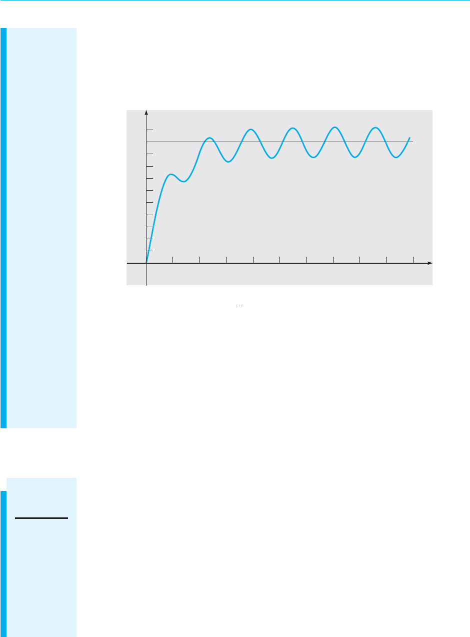
August 7, 2012 21:03 c02 Sheet number 28 Page number 58 cyan black
58 Chapter 2. First Order Differential Equations
A plot of the solution (24) is shown in Figure 2.3.3,along with the line q = 20. The exponential
term in the solution is important for small t, but it diminishes rapidly as t increases. Later, the
solution consists of an oscillation, due to the sin 2t and cos 2t terms, about the constant level
q = 20. Note that if the sin 2t term were not present in Eq. (21), then q = 20 would be the
equilibrium solution of that equation.
2
22
20
18
16
14
12
10
8
4
6
2
8 1046
t
12 14 16 18 20
q
FIGURE 2.3.3 Solution of the initial value problem (21), (22):
dq/dt +
1
2
q = 10 + 5 sin 2t, q(0) = 0.
Let us now consider the adequacy of the mathematical model itself for this problem.
The model rests on several assumptions that have not yet been stated explicitly. In the first
place, the amount of water in the pond is controlled entirely by the rates of flow in and out—
none is lost by evaporation or by seepage into the ground, and none is gained by rainfall.
The same is true of the chemical; it flows into and out of the pond, but none is absorbed by
fish or other organisms living in the pond. In addition, we assume that the concentration of
chemical in the pond is uniform throughout the pond. Whether the results obtained from the
model are accurate depends strongly on the validity of these simplifying assumptions.
EXAMPLE
4
Escape
Velocity
A body of constant mass m is projected away from the earth in a direction perpendicular to the
earth’s surface with an initial velocity v
0
. Assuming that there is no air resistance, but taking
into account the variation of the earth’s gravitational field with distance, find an expression
for the velocity during the ensuing motion. Also find the initial velocity that is required to
lift the body to a given maximum altitude ξ above the surface of the earth, and find the
least initial velocity for which the body will not return to the earth; the latter is the escape
velocity.
Let the positive x-axis point away from the center of the earth along the line of motion with
x = 0 lying on the earth’s surface; see Figure 2.3.4. The figure is drawn horizontally to remind
you that gravity is directed toward the center of the earth, which is not necessarily downward
from a perspective away from the earth’s surface. The gravitational force acting on the body
(that is, its weight) is inversely proportional to the square of the distance from the center of
the earth and is given by w(x) =−k/(x + R)
2
, where k is a constant, R is the radius of the
earth, and the minus sign signifies that w(x) is directed in the negative x direction. We know

August 7, 2012 21:03 c02 Sheet number 29 Page number 59 cyan black
2.3 Modeling with First Order Equations 59
x
m
mgR
2
(R + x)
2
R
FIGURE 2.3.4 A body in the earth’s gravitational field.
that on the earth’s surface w(0) is given by −mg, where g is the acceleration due to gravity at
sea level. Therefore, k = mgR
2
and
w(x) =−
mgR
2
(R + x)
2
. (25)
Since there are no other forces acting on the body, the equation of motion is
m
dv
dt
=−
mgR
2
(R + x)
2
, (26)
and the initial condition is
v(0) = v
0
. (27)
Unfortunately, Eq. (26) involves too many variables since it depends on t, x, and v.To
remedy this situation, we can eliminate t from Eq. (26) by thinking of x, rather than t, as the
independent variable. Then we can express dv/dt in terms of dv/dx by using the chain rule;
hence
dv
dt
=
dv
dx
dx
dt
= v
dv
dx
,
and Eq. (26) is replaced by
v
dv
dx
=−
gR
2
(R + x)
2
. (28)
Equation (28) is separable but not linear, so by separating the variables and integrating, we
obtain
v
2
2
=
gR
2
R + x
+ c. (29)
Since x = 0 when t = 0,the initial condition (27) at t = 0 can be replaced by the condition that
v = v
0
when x = 0. Hence c = (v
2
0
/2) − gR and
v =±
+
v
2
0
− 2gR +
2gR
2
R + x
. (30)
Note that Eq. (30) gives the velocity as a function of altitude rather than as a function of time.
The plus sign must be chosen if the body is rising, and the minus sign must be chosen if it is
falling back to earth.
To determine the maximum altitude ξ that the body reaches, we set v = 0 and x = ξ in
Eq. (30) and then solve for ξ, obtaining
ξ =
v
2
0
R
2gR − v
2
0
. (31)

August 7, 2012 21:03 c02 Sheet number 30 Page number 60 cyan black
60 Chapter 2. First Order Differential Equations
Solving Eq. (31) for v
0
, we find the initial velocity required to lift the body to the altitude ξ,
namely,
v
0
=
+
2gR
ξ
R + ξ
. (32)
The escape velocity v
e
is then found by letting ξ →∞. Consequently,
v
e
=
!
2gR. (33)
The numerical value of v
e
is approximately 6.9 mi/s, or 11.1 km/s.
The preceding calculation of the escape velocity neglects the effect of air resistance, so the
actual escape velocity (including the effect of air resistance) is somewhat higher. On the other
hand, the effective escape velocity can be significantly reduced if the body is transported a
considerable distance above sea level before being launched. Both gravitational and frictional
forces are thereby reduced;air resistance,in particular,diminishes quite rapidly withincreasing
altitude. You should keep in mind also that it may well be impractical to impart too large an
initial velocity instantaneously; space vehicles, for instance, receive their initial acceleration
during a period of a few minutes.
PROBLEMS 1. Consider a tank used in certain hydrodynamic experiments. After one experiment the
tank contains 200 L of a dye solution with a concentration of 1 g/L. To prepare for
the next experiment, the tank is to be rinsed with fresh water flowing in at a rate of
2 L/min, the well-stirred solution flowing out at the same rate. Find the time that will
elapse before the concentration of dye in the tank reaches 1% of its original value.
2. A tank initially contains 120 L of pure water. A mixture containing a concentration of
γ g/L of salt enters the tank at a rate of 2 L/min, and the well-stirred mixture leaves the
tank at the same rate. Find an expression in terms of γ for the amount of salt in the tank
at any time t. Also find the limiting amount of salt in the tank as t →∞.
3. A tank originally contains 100 gal of fresh water. Then water containing
1
2
lb of salt per
gallon is poured into the tank at a rate of 2 gal/min, and the mixture is allowed to leave at
the same rate.After 10 min the process is stopped, and fresh water is poured into the tank
at a rate of 2 gal/min, with the mixture again leaving at the same rate. Find the amount of
salt in the tank at the end of an additional 10 min.
4. A tank with a capacity of 500 gal originally contains 200 gal of water with 100 lb of salt
in solution. Water containing 1 lb of salt per gallon is entering at a rate of 3 gal/min, and
the mixture is allowed to flow out of the tank at a rate of 2 gal/min. Find the amount
of salt in the tank at any time prior to the instant when the solution begins to overflow.
Find the concentration (in pounds per gallon) of salt in the tank when it is on the point
of overflowing. Compare this concentration with the theoretical limiting concentration if
the tank had infinite capacity.
5.
A tank contains 100 gal of water and 50 oz of salt.Water containing a salt concentration of
1
4
(1 +
1
2
sin t) oz/gal flows into the tank at a rate of 2 gal/min, and the mixture in the tank
flows out at the same rate.
(a) Find the amount of salt in the tank at any time.
(b) Plot the solution for a time period long enough so that you see the ultimate behavior
of the graph.
(c) The long-time behavior of the solution is an oscillation about a certain constant level.
What is this level? What is the amplitude of the oscillation?

August 7, 2012 21:03 c02 Sheet number 31 Page number 61 cyan black
2.3 Modeling with First Order Equations 61
6. Suppose that a tank containing a certain liquid has an outlet near the bottom. Let h(t)
be the height of the liquid surface above the outlet at time t. Torricelli’s
2
principle states
that the outflow velocity v at the outlet is equal to the velocity of a particle falling freely
(with no drag) from the height h.
(a) Show that v =
!
2gh, where g is the acceleration due to gravity.
(b) By equating the rate of outflow to the rate of change of liquid in the tank, show that
h(t) satisfies the equation
A(h)
dh
dt
=−αa
!
2gh, (i)
where A(h) is the area of the cross section of the tank at height h and a is the area of the
outlet. The constant α is a contraction coefficient that accounts for the observed fact that
the cross section of the (smooth) outflow stream is smaller than a. The value of α for water
is about 0.6.
(c) Consider a water tank in the form of a right circular cylinder that is 3 m high above
the outlet. The radius of the tank is 1 m, and the radius of the circular outlet is 0.1 m.
If the tank is initially full of water, determine how long it takes to drain the tank down to
the level of the outlet.
7. Suppose that a sum S
0
is invested at an annual rate of return r compounded continuously.
(a) Find the time T required for the original sum to double in value as a function of r.
(b) Determine T if r = 7%.
(c) Find the return rate that must be achieved if the initial investment is to double in
8 years.
8. A young person with no initial capital invests k dollars per year at an annual rate of
return r. Assume that investments are made continuously and that the return is
compounded continuously.
(a) Determine the sum S(t) accumulated at any time t.
(b) If r = 7.5%,determine k so that $1 million will be available for retirement in 40 years.
(c) If k = $2000/year,determine the return rate r that must be obtained to have $1 million
available in 40 years.
9. A certain college graduate borrows $8000 to buy a car. The lender charges interest at
an annual rate of 10%. Assuming that interest is compounded continuously and that
the borrower makes payments continuously at a constant annual rate k, determine the
payment rate k that is required to pay off the loan in 3 years. Also determine how much
interest is paid during the 3-year period.
10. A home buyer can afford to spend no more than $1500/month on mortgage payments.
Suppose that the interest rate is 6%, that interest is compounded continuously, and that
payments are also made continuously.
(a) Determine the maximum amount that this buyer can afford to borrow on a 20-year
mortgage; on a 30-year mortgage.
(b) Determine the total interest paid during the term of the mortgage in each of the cases
in part (a).
2
Evangelista Torricelli (1608–1647), successor to Galileo as court mathematician in Florence, published
this result in 1644. He is also known for constructing the first mercury barometer and for making important
contributions to geometry.

August 7, 2012 21:03 c02 Sheet number 32 Page number 62 cyan black
62 Chapter 2. First Order Differential Equations
11. A home buyer wishes to borrow $250,000 at an interest rate of 6% to finance the pur-
chase.Assume that interest is compounded continuously and that payments are also made
continuously.
(a) Determine the monthly payment that is required to pay off the loan in 20 years;
in 30 years.
(b) Determine the total interest paid during the term of the loan in each of the cases in
part (a).
12.
A recent college graduate borrows $150,000 at an interest rate of 6% to purchase a con-
dominium. Anticipating steady salary increases, the buyer expects to make payments at a
monthly rate of 800 + 10t, where t is the number of months since the loan was made.
(a) Assuming that this payment schedule can be maintained, when will the loan be fully
paid?
(b) Assuming the same payment schedule, how large a loan could be paid off in exactly
20 years?
13. An important tool in archeological research is radiocarbon dating, developed by the
American chemistWillard F. Libby.
3
This is a means ofdetermining theage of certain wood
and plant remains, and hence of animal or human bones or artifacts found buried at the
same levels. Radiocarbon dating is based on the fact that some wood or plant remains con-
tain residual amounts of carbon-14,aradioactive isotope of carbon.This isotope is accumu-
lated during the lifetime of the plant and begins to decay at its death. Since the half-life of
carbon-14 is long (approximately 5730 years
4
), measurable amounts of carbon-14 remain
after many thousands of years. If even a tiny fraction of the original amount of carbon-14
is still present, then by appropriate laboratory measurements the proportion of the orig-
inal amount of carbon-14 that remains can be accurately determined. In other words, if
Q(t) is the amount of carbon-14 at time t and Q
0
is the original amount, then the ratio
Q(t)/Q
0
can be determined,as long as this quantity is not too small. Present measurement
techniques permit the use of this method for time periods of 50,000 years or more.
(a) Assuming that Q satisfies the differential equation Q
′
=−rQ, determine the decay
constant r for carbon-14.
(b) Find an expression for Q(t) at any time t, if Q(0) = Q
0
.
(c) Suppose that certain remains are discovered in which the current residual amount of
carbon-14 is 20% of the original amount. Determine the age of these remains.
14.
Suppose that a certain population has a growth rate that varies with time and that this
population satisfies the differential equation
dy/dt = (0.5 + sin t)y/5.
(a) If y(0) = 1, find (or estimate) the time τ at which the population has doubled. Choose
other initial conditions and determine whether the doubling time τ depends on the initial
population.
(b) Suppose that the growth rate is replaced by its average value 1/10. Determine the
doubling time τ in this case.
3
Willard F. Libby (1908–1980) was born in rural Colorado and received his education at the University of
California at Berkeley. He developed the method of radiocarbon dating beginning in 1947 while he was
at the University of Chicago. For this work he was awarded the Nobel Prize in chemistry in 1960.
4
McGraw-Hill Encyclopedia of Science and Technology (8th ed.) (New York: McGraw-Hill, 1997), Vol. 5,
p. 48.

August 7, 2012 21:03 c02 Sheet number 33 Page number 63 cyan black
2.3 Modeling with First Order Equations 63
(c) Suppose that the term sin t in the differential equation is replaced by sin 2πt; that is,
the variation in the growth rate has a substantially higher frequency. What effect does this
have on the doubling time τ?
(d) Plot the solutions obtained in parts (a), (b), and (c) on a single set of axes.
15.
Suppose that a certain population satisfies the initial value problem
dy/dt = r(t)y − k, y(0) = y
0
,
where the growth rate r(t) is given by r(t) = (1 + sin t)/5, and k represents the rate of
predation.
(a) Suppose that k = 1/5. Plot y versus t for several values of y
0
between 1/2 and 1.
(b) Estimate the critical initial population y
c
below which the population will become
extinct.
(c) Choose other values of k and find the corresponding y
c
for each one.
(d) Use the data you have found in parts (b) and (c) to plot y
c
versus k.
16. Newton’s law of cooling states that the temperature of an object changes at a rate pro-
portional to the difference between its temperature and that of its surroundings. Suppose
that the temperature of a cup of coffee obeys Newton’s law of cooling. If the coffee has a
temperature of 200
◦
F when freshly poured, and 1 min later has cooled to 190
◦
F in a room
at 70
◦
F, determine when the coffee reaches a temperature of 150
◦
F.
17.
Heat transfer from a body to its surroundings by radiation, based on the Stefan–
Boltzmann
5
law, is described by the differential equation
du
dt
=−α(u
4
− T
4
), (i)
where u(t) is the absolute temperature of the body at time t, T is the absolute temperature
of the surroundings, and α is a constant depending on the physical parameters of the body.
However, if u is much larger than T, then solutions of Eq. (i) are well approximated by
solutions of the simpler equation
du
dt
=−αu
4
. (ii)
Suppose that a body with initial temperature 2000 K is surrounded by a medium with
temperature 300 K and that α = 2.0 × 10
−12
K
−3
/s.
(a) Determine the temperature of the body at any time by solving Eq. (ii).
(b) Plot the graph of u versus t.
(c) Find the time τ at which u(τ) = 600—that is,twice the ambient temperature. Up to this
time the error in using Eq. (ii) to approximate the solutions of Eq. (i) is no more than 1%.
18.
Consider an insulated box (a building,perhaps) with internal temperature u(t). According
to Newton’s law of cooling, u satisfies the differential equation
du
dt
=−k[u − T(t)], (i)
where T(t) is the ambient (external) temperature. Suppose that T(t) varies sinusoidally;
for example, assume that T(t) = T
0
+ T
1
cos ωt.
5
Jozef Stefan (1835–1893), professor of physics at Vienna, stated the radiation law on empirical grounds
in 1879. His student Ludwig Boltzmann (1844–1906) derived it theoretically from the principles of
thermodynamics in 1884. Boltzmann is best known for his pioneering work in statistical mechanics.

August 7, 2012 21:03 c02 Sheet number 34 Page number 64 cyan black
64 Chapter 2. First Order Differential Equations
(a) Solve Eq. (i) and express u(t) in terms of t, k, T
0
, T
1
, and ω. Observe that part of
your solution approaches zero as t becomes large; this is called the transient part. The
remainder of the solution is called the steady state; denote it by S(t).
(b) Suppose that t is measured in hours and that ω = π/12, corresponding to a period of
24 h for T(t). Further, let T
0
= 60
◦
F, T
1
= 15
◦
F, and k = 0.2/h. Draw graphs of S(t) and
T(t) versus t on the same axes. From your graph estimate the amplitude R of the oscillatory
part of S(t). Also estimate the time lag τ between corresponding maxima of T(t) and S(t).
(c) Let k, T
0
, T
1
, and ω now be unspecified. Write the oscillatory part of S(t) in the form
R cos[ω(t − τ)]. Use trigonometric identities to find expressions for R and τ. Let T
1
and ω
have the values given in part (b), and plot graphs of R and τ versus k.
19. Consider a lake of constant volume V containing at time t an amount Q(t) of pollutant,
evenly distributed throughout the lake with a concentration c(t), where c(t) = Q(t)/V.
Assume that water containing a concentration k of pollutant enters the lake at a rate r,
and that water leaves the lake at the same rate. Suppose that pollutants are also added
directly to the lake at a constant rate P. Note that the given assumptions neglect a number
of factors that may, in some cases, be important—for example, the water added or lost
by precipitation, absorption, and evaporation; the stratifying effect of temperature differ-
ences in a deep lake; the tendency of irregularities in the coastline to produce sheltered
bays;and the fact that pollutants are deposited unevenly throughout the lake but (usually)
at isolated points around its periphery. The results below must be interpreted in the light
of the neglect of such factors as these.
(a) If at time t = 0 the concentration of pollutant is c
0
, find an expression for the
concentration c(t) at any time. What is the limiting concentration as t →∞?
(b) If the addition of pollutants to the lake is terminated (k = 0 and P = 0 for t > 0),
determine the time interval T that must elapse before the concentration of pollutants is
reduced to 50% of its original value; to 10% of its original value.
(c) Table 2.3.2 contains data
6
for several of the Great Lakes. Using these data, determine
from part (b) the time T that is needed to reduce the contamination of each of these lakes
to 10% of the original value.
TABLE 2.3.2 Volume and Flow Data for the Great
Lakes
Lake V (km
3
× 10
3
) r (km
3
/year)
Superior 12.2 65.2
Michigan 4.9 158
Erie 0.46 175
Ontario 1.6 209
20. A ball with mass 0.15 kg is thrown upward with initial velocity 20 m/s from the roof of a
building 30 m high. Neglect air resistance.
(a) Find the maximum height above the ground that the ball reaches.
(b) Assuming that the ball misses the building on the way down, find the time that it hits
the ground.
(c) Plot the graphs of velocity and position versus time.
6
This problem is based on R. H. Rainey, “Natural Displacement of Pollution from the Great Lakes,”
Science 155 (1967), pp. 1242–1243; the information in the table was taken from that source.

August 7, 2012 21:03 c02 Sheet number 35 Page number 65 cyan black
2.3 Modeling with First Order Equations 65
21. Assume that the conditions are as in Problem 20 except that there is a force due to air
resistance of magnitude |v|/30 directed opposite to the velocity, where the velocity v is
measured in m/s.
(a) Find the maximum height above the ground that the ball reaches.
(b) Find the time that the ball hits the ground.
(c) Plot the graphs of velocity and position versus time. Compare these graphs with the
corresponding ones in Problem 20.
22.
Assume that the conditions are as in Problem 20 except that there is a force due to air
resistance of magnitude v
2
/1325 directed opposite to the velocity, where the velocity v is
measured in m/s.
(a) Find the maximum height above the ground that the ball reaches.
(b) Find the time that the ball hits the ground.
(c) Plot the graphs of velocity and position versus time. Compare these graphs with the
corresponding ones in Problems 20 and 21.
23.
A skydiver weighing 180 lb (including equipment) falls vertically downward from an alti-
tude of 5000 ft and opens the parachute after 10 s of free fall. Assume that the force
of air resistance, which is directed opposite to the velocity, is of magnitude 0.75|v| when
the parachute is closed and is of magnitude 12|v| when the parachute is open, where the
velocity v is measured in ft/s.
(a) Find the speed of the skydiver when the parachute opens.
(b) Find the distance fallen before the parachute opens.
(c) What is the limiting velocity v
L
after the parachute opens?
(d) Determine how long the sky diver is in the air after the parachute opens.
(e) Plot the graph of velocity versus time from the beginning of the fall until the skydiver
reaches the ground.
24. A rocket sled having an initial speed of 150 mi/h is slowed by a channel of water. Assume
that during the braking process, the acceleration a is given by a(v) =−µv
2
, where v is the
velocity and µ is a constant.
(a) As in Example 4 in the text, use the relation dv/dt = v(dv/dx) to write the equation
of motion in terms of v and x.
(b) If it requires a distance of 2000 ft to slow the sled to 15 mi/h, determine the value of µ.
(c) Find the time τ required to slow the sled to 15 mi/h.
25. A body of constant mass m is projected vertically upward with an initial velocity v
0
in a medium offering a resistance k|v|, where k is a constant. Neglect changes in the
gravitational force.
(a) Find the maximum height x
m
attained by the body and the time t
m
at which this
maximum height is reached.
(b) Show that if kv
0
/mg < 1, then t
m
and x
m
can be expressed as
t
m
=
v
0
g
,
1 −
1
2
kv
0
mg
+
1
3
'
kv
0
mg
(
2
−···
-
,
x
m
=
v
2
0
2g
,
1 −
2
3
kv
0
mg
+
1
2
'
kv
0
mg
(
2
−···
-
.
(c) Show that the quantity kv
0
/mg is dimensionless.
26. A body of mass m is projected vertically upward with an initial velocity v
0
in a medium
offering a resistance k|v|, where k is a constant. Assume that the gravitational attraction
of the earth is constant.
(a) Find the velocity v(t) of the body at any time.

August 7, 2012 21:03 c02 Sheet number 36 Page number 66 cyan black
66 Chapter 2. First Order Differential Equations
(b) Use the result of part (a) to calculate the limit of v(t) as k → 0—that is, as the resis-
tance approaches zero. Does this result agree with the velocity of a mass m projected
upward with an initial velocity v
0
in a vacuum?
(c) Use the result of part (a) to calculate the limit of v(t) as m → 0—that is, as the mass
approaches zero.
27. A body falling in a relatively dense fluid, oil for example, is acted on by three forces
(see Figure 2.3.5): a resistive force R, a buoyant force B, and its weight w due to gravity.
The buoyant force is equal to the weight of the fluid displaced by the object. For a slowly
moving spherical body of radius a,the resistive force is given by Stokes’s law,R = 6πµa|v|,
where v is the velocity of the body, and µ is the coefficient of viscosity of the surrounding
fluid.
7
(a) Find the limiting velocity of a solid sphere of radius a and density ρ falling freely in a
medium of density ρ
′
and coefficient of viscosity µ.
(b) In 1910 R. A. Millikan
8
studied the motion of tiny droplets of oil falling in an electric
field. A field of strength E exerts a force Ee on a droplet with charge e. Assume that E
has been adjusted so the droplet is held stationary (v = 0) and that w and B are as given
above. Find an expression for e. Millikan repeated this experiment many times, and from
the data that he gathered he was able to deduce the charge on an electron.
R
w
a
B
FIGURE 2.3.5 A body falling in a dense fluid.
28.
A mass of 0.25 kg is dropped from rest in a medium offering a resistance of 0.2|v|, where
v is measured in m/s.
(a) If the mass is dropped from a height of 30 m, find its velocity when it hits the ground.
(b) If the mass is to attain a velocity of no more than 10 m/s, find the maximum height
from which it can be dropped.
7
Sir George Gabriel Stokes (1819–1903) was born in Ireland but for most of his life was at Cambridge
University, first as a student and later as a professor. Stokes was one of the foremost applied mathemati-
cians of the nineteenth century, best known for his work in fluid dynamics and the wave theory of light.
The basic equations of fluid mechanics (the Navier–Stokes equations) are named partly in his honor, and
one of the fundamental theorems of vector calculus bears his name. He was also one of the pioneers in
the use of divergent (asymptotic) series.
8
Robert A. Millikan (1868–1953) was educated at Oberlin College and Columbia University. Later he
was a professor at the University of Chicago and California Institute of Technology. His determination of
the charge on an electron was published in 1910. For this work, and for other studies of the photoelectric
effect, he was awarded the Nobel Prize for Physics in 1923.

August 7, 2012 21:03 c02 Sheet number 37 Page number 67 cyan black
2.3 Modeling with First Order Equations 67
(c) Suppose that the resistive force is k|v|, where v is measured in m/s and k is a constant.
If the mass is dropped from a height of 30 m and must hit the ground with a velocity of
no more than 10 m/s, determine the coefficient of resistance k that is required.
29. Suppose that a rocket is launched straight up from the surface of the earth with initial
velocity v
0
=
!
2gR, where R is the radius of the earth. Neglect air resistance.
(a) Find an expression for the velocity v in terms of the distance x from the surface of the
earth.
(b) Find the time required for the rocket to go 240,000 mi (the approximate distance from
the earth to the moon). Assume that R = 4000 mi.
30.
Let v(t) and w(t) be the horizontal and vertical components,respectively, of the velocity of
a batted (or thrown) baseball. In the absence of air resistance,v and w satisfy the equations
dv/dt = 0, dw/dt =−g.
(a) Show that
v = u cos A, w =−gt + u sin A,
where u is the initial speed of the ball and A is its initial angle of elevation.
(b) Let x(t) and y(t) be the horizontal and vertical coordinates, respectively, of the ball at
time t. If x(0) = 0 and y(0) = h, find x(t) and y(t) at any time t.
(c) Let g = 32 ft/s
2
, u = 125 ft/s, and h = 3 ft. Plot the trajectory of the ball for several
values of the angle A; that is, plot x(t) and y(t) parametrically.
(d) Suppose the outfield wall is at a distance L and has height H. Find a relation between
u and A that must be satisfied if the ball is to clear the wall.
(e) Suppose that L = 350 ft and H = 10 ft. Using the relation in part (d),find (or estimate
from a plot) the range of values of A that correspond to an initial velocity of u = 110 ft/s.
(f) For L = 350 and H = 10, find the minimum initial velocity u and the corresponding
optimal angle A for which the ball will clear the wall.
31.
A more realistic model (than that in Problem 30) of a baseball in flight includes the effect
of air resistance. In this case the equations of motion are
dv/dt =−rv, dw/dt =−g − rw,
where r is the coefficient of resistance.
(a) Determine v(t) and w(t) in terms of initial speed u and initial angle of elevation A.
(b) Find x(t) and y(t) if x(0) = 0 and y(0) = h.
(c) Plot the trajectory of the ball for r = 1/5, u = 125, h = 3, and for several values of A.
How do the trajectories differ from those in Problem 31 with r = 0?
(d) Assuming that r = 1/5 and h = 3, find the minimum initial velocity u and the optimal
angle A for which the ball will clear a wall that is 350 ft distant and 10 ft high. Compare
this result with that in Problem 30(f).
32. Brachistochrone Problem. One of the famous problems in the history of mathematics is
the brachistochrone
9
problem: to find the curve along which a particle will slide without
friction in the minimum time from one given point P to another Q, the second point being
lower than the first but not directly beneath it (see Figure 2.3.6). This problem was posed
by Johann Bernoulli in 1696 as a challenge problem to the mathematicians of his day.
9
The word “brachistochrone” comes from the Greek words brachistos, meaning shortest, and chronos,
meaning time.

August 7, 2012 21:03 c02 Sheet number 38 Page number 68 cyan black
68 Chapter 2. First Order Differential Equations
Correct solutions were found by Johann Bernoulli and his brother Jakob Bernoulli and
by Isaac Newton, Gottfried Leibniz, and the Marquis de L’Hôpital. The brachistochrone
problem is important in the development of mathematics as one of the forerunners of the
calculus of variations.
In solving this problem, it is convenient to take the origin as the upper point P and to
orient the axes as shown in Figure 2.3.6. The lower point Q has coordinates (x
0
, y
0
).Itis
then possible to show that the curve of minimum time is given by a function y = φ(x) that
satisfies the differential equation
(1 + y
′2
)y = k
2
, (i)
where k
2
is a certain positive constant to be determined later.
(a) Solve Eq. (i) for y
′
. Why is it necessary to choose the positive square root?
(b) Introduce the new variable t by the relation
y = k
2
sin
2
t. (ii)
Show that the equation found in part (a) then takes the form
2k
2
sin
2
tdt = dx. (iii)
(c) Letting θ = 2t,showthat the solutionof Eq.(iii) for whichx = 0 when y = 0 isgiven by
x = k
2
(θ − sin θ)/2, y = k
2
(1 − cos θ)/2. (iv)
Equations (iv) are parametric equations of the solution of Eq. (i) that passes through
(0, 0). The graph of Eqs. (iv) is called a cycloid.
(d) If we make a proper choice of the constant k, then the cycloid also passes through the
point(x
0
, y
0
) and is the solution ofthe brachistochrone problem. Findk if x
0
= 1and y
0
= 2.
x
P
y
Q(x
0
, y
0
)
FIGURE 2.3.6 The brachistochrone.
2.4 Differences Between Linear and Nonlinear Equations
Up to now, we have been primarily concerned with showing that first order differ-
ential equations can be used to investigate many different kinds of problems in the
natural sciences, and with presenting methods of solving such equations if they are
either linear or separable. Now it is time to turn our attention to some more general

August 7, 2012 21:03 c02 Sheet number 39 Page number 69 cyan black
2.4 Differences Between Linear and Nonlinear Equations 69
questions about differential equations and to explore in more detail some important
ways in which nonlinear equations differ from linear ones.
Existence and Uniqueness of Solutions. So far,we have discussed a number ofinitial value
problems, each of which had a solution and apparently only one solution. That raises
the question of whether this is true of all initial value problems for first order equa-
tions. In other words, does every initial value problem have exactly one solution?
This may be an important question even for nonmathematicians. If you encounter
an initial value problem in the course of investigating some physical problem, you
might want to know that it has a solution before spending very much time and effort
in trying to find it. Further, if you are successful in finding one solution, you might
be interested in knowing whether you should continue a search for other possible
solutions or whether you can be sure that there are no other solutions. For linear
equations, the answers to these questions are given by the following fundamental
theorem.
Theorem 2.4.1
If the functions p and g are continuous on an open interval I: α<t <βcontain-
ing the point t = t
0
, then there exists a unique function y = φ(t) that satisfies the
differential equation
y
′
+ p(t)y = g(t) (1)
for each t in I, and that also satisfies the initial condition
y(t
0
) = y
0
, (2)
where y
0
is an arbitrary prescribed initial value.
ObservethatTheorem 2.4.1 states that thegiven initial value problemhas asolution
and also that the problem has only one solution. In other words, the theorem asserts
both the existence and the uniqueness of the solution of the initial value problem (1),
(2). In addition, it states that the solution exists throughout any interval I containing
the initial point t
0
in which the coefficients p and g are continuous.That is,the solution
can be discontinuous or fail to exist only at points where at least one of p and g is
discontinuous. Such points can often be identified at a glance.
The proof ofthis theorem is partly contained in the discussion in Section 2.1leading
to the formula [Eq. (32) in Section 2.1]
µ(t)y =
"
µ(t)g(t) dt + c, (3)
where [Eq. (30) in Section 2.1]
µ(t) = exp
"
p(t) dt. (4)
The derivation in Section 2.1 shows that if Eq. (1) has a solution, then it must be
given by Eq. (3). By looking slightly more closely at that derivation, we can also
conclude that the differential equation (1) must indeed have a solution. Since p is

August 7, 2012 21:03 c02 Sheet number 40 Page number 70 cyan black
70 Chapter 2. First Order Differential Equations
continuous for α<t <β, it follows that µ is defined in this interval and is a nonzero
differentiable function. Upon multiplying Eq. (1) by µ(t), we obtain
[µ(t)y]
′
= µ(t)g(t). (5)
Since both µ and g are continuous, the function µg is integrable, and Eq. (3) follows
from Eq. (5). Further, the integral of µg is differentiable, so y as given by Eq. (3)
exists and is differentiable throughout the interval α<t <β. By substituting the
expression for y from Eq. (3) into either Eq. (1) or Eq. (5), you can verify that
this expression satisfies the differential equation throughout the interval α<t <β.
Finally, the initial condition (2) determines the constant c uniquely, so there is only
one solution of the initial value problem; this completes the proof.
Equation (4) determines the integrating factor µ(t) only up to a multiplicative
factor that depends on the lower limit of integration. If we choose this lower limit to
be t
0
, then
µ(t) = exp
"
t
t
0
p(s) ds, (6)
and it follows that µ(t
0
) = 1. Using the integrating factor given by Eq. (6), and choos-
ing the lower limit of integration in Eq. (3) also to be t
0
,we obtain the general solution
of Eq. (1) in the form
y =
1
µ(t)
%
"
t
t
0
µ(s)g (s ) ds + c
&
. (7)
To satisfy the initial condition (2), we must choose c = y
0
. Thus the solution of the
initial value problem (1), (2) is
y =
1
µ(t)
%
"
t
t
0
µ(s)g (s ) ds + y
0
&
, (8)
where µ(t) is given by Eq. (6).
Turning now to nonlinear differential equations, we must replace Theorem 2.4.1
by a more general theorem, such as the one that follows.
Theorem 2.4.2
Let the functions f and ∂f /∂y be continuous in some rectangle α<t <β,
γ<y <δcontaining the point (t
0
, y
0
). Then, in some interval t
0
− h < t < t
0
+ h
contained in α<t <β, there is a unique solution y = φ(t) of the initial value
problem
y
′
= f (t, y), y(t
0
) = y
0
. (9)
Observe that the hypotheses in Theorem 2.4.2 reduce to those in Theorem 2.4.1 if
the differential equation is linear. In this case
f (t, y) =−p(t)y + g(t) and ∂f (t, y)/∂y =−p(t),
so the continuity of f and ∂f /∂y is equivalent to the continuity of p and g.
The proof of Theorem 2.4.1 was comparatively simple because it could be based
on the expression (3) that gives the solution of an arbitrary linear equation. There
is no corresponding expression for the solution of the differential equation (9), so

August 7, 2012 21:03 c02 Sheet number 41 Page number 71 cyan black
2.4 Differences Between Linear and Nonlinear Equations 71
the proof of Theorem 2.4.2 is much more difficult. It is discussed to some extent in
Section 2.8 and in greater depth in more advanced books on differential equations.
Here we note thatthe conditionsstated inTheorem2.4.2 aresufficient toguarantee
the existence of a unique solution of the initial value problem (9) in some interval
t
0
− h < t < t
0
+ h, but they are not necessary. That is, the conclusion remains true
under slightly weaker hypotheses about the function f . In fact, the existence of a
solution (but not its uniqueness) can be established on the basis of the continuity of
f alone.
An important geometrical consequence of the uniqueness parts of Theorems 2.4.1
and 2.4.2 is that the graphs of two solutions cannot intersect each other. Otherwise,
there would be two solutions that satisfy the initial condition corresponding to the
point of intersection, in contradiction to Theorem 2.4.1 or 2.4.2.
We now consider some examples.
EXAMPLE
1
Use Theorem 2.4.1 to find an interval in which the initial value problem
ty
′
+ 2y = 4t
2
, (10)
y(1) = 2 (11)
has a unique solution.
Rewriting Eq. (10) in the standard form (1), we have
y
′
+ (2/t)y = 4t,
so p(t) = 2/t and g(t) = 4t.Thus,for this equation,g is continuous for all t,while p is continuous
only for t < 0 or for t > 0. The interval t > 0 contains the initial point; consequently,Theorem
2.4.1 guarantees that the problem (10), (11) has a unique solution on the interval 0 < t < ∞.
In Example 4 of Section 2.1 we found the solution of this initial value problem to be
y = t
2
+
1
t
2
, t > 0. (12)
Now suppose that the initial condition (11) is changed to y(−1) = 2. Then Theorem 2.4.1
asserts the existence of a unique solution for t < 0. As you can readily verify, the solution is
again given by Eq. (12), but now on the interval −∞ < t < 0.
EXAMPLE
2
Apply Theorem 2.4.2 to the initial value problem
dy
dx
=
3x
2
+ 4x + 2
2(y − 1)
, y(0) =−1. (13)
Note that Theorem 2.4.1 is not applicable to this problem since the differential equation is
nonlinear. To apply Theorem 2.4.2, observe that
f (x, y) =
3x
2
+ 4x + 2
2(y − 1)
,
∂f
∂y
(x, y) =−
3x
2
+ 4x + 2
2(y − 1)
2
.
Thuseach of these functions is continuous everywhere except on the line y = 1. Consequently,a
rectangle can be drawn about the initial point (0, −1) in which both f and ∂f /∂y are continuous.
Therefore, Theorem 2.4.2 guarantees that the initial value problem has a unique solution in
some interval about x = 0. However, even though the rectangle can be stretched infinitely
far in both the positive and the negative x directions, this does not necessarily mean that the
solution exists for all x. Indeed, the initial value problem (13) was solved in Example 2 of
Section 2.2, and the solution exists only for x > −2.

August 7, 2012 21:03 c02 Sheet number 42 Page number 72 cyan black
72 Chapter 2. First Order Differential Equations
Now suppose we change the initial condition to y(0) = 1. The initial point now lies on the
line y = 1, so no rectangle can be drawn about it within which f and ∂f /∂y are continuous.
Consequently, Theorem 2.4.2 says nothing about possible solutions of this modified problem.
However, if we separate the variables and integrate, as in Section 2.2, we find that
y
2
− 2y = x
3
+ 2x
2
+ 2x + c.
Further, if x = 0 and y = 1, then c =−1. Finally, by solving for y, we obtain
y = 1 ±
!
x
3
+ 2x
2
+ 2x. (14)
Equation (14) provides two functions that satisfy the given differential equation for x > 0 and
also satisfy the initial condition y(0) = 1.
EXAMPLE
3
Consider the initial value problem
y
′
= y
1/3
, y(0) = 0 (15)
for t ≥ 0. Apply Theorem 2.4.2 to this initial value problem and then solve the problem.
The function f (t, y) = y
1/3
is continuous everywhere, but ∂f /∂y does not exist when y = 0,
and hence it is not continuous there. Thus Theorem 2.4.2 does not apply to this problem, and
no conclusion can be drawn from it. However, by the remark following Theorem 2.4.2, the
continuity of f does ensure the existence of solutions, though not their uniqueness.
To understand the situation more clearly, we must actually solve the problem, which is easy
to do since the differential equation is separable. Thus we have
y
−1/3
dy = dt,
so
3
2
y
2/3
= t + c
and
y =
.
2
3
(t + c)
/
3/2
.
The initial condition is satisfied if c = 0, so
y = φ
1
(t) =
0
2
3
t
1
3/2
, t ≥ 0 (16)
satisfies both of Eqs. (15). On the other hand, the function
y = φ
2
(t) =−
0
2
3
t
1
3/2
, t ≥ 0 (17)
is also a solution of the initial value problem. Moreover, the function
y = ψ(t) = 0, t ≥ 0 (18)
is yet another solution. Indeed, for an arbitrary positive t
0
, the functions
y = χ(t) =
2
0, if 0 ≤ t < t
0
,
±
.
2
3
(t − t
0
)
/
3/2
,ift ≥ t
0
(19)
are continuous, are differentiable (in particular at t = t
0
), and are solutions of the initial value
problem (15). Hence this problem has an infinite family of solutions; see Figure 2.4.1, where a
few of these solutions are shown.

August 7, 2012 21:03 c02 Sheet number 43 Page number 73 cyan black
2.4 Differences Between Linear and Nonlinear Equations 73
As already noted,thenonuniqueness of the solutions of the problem (15)does not contradict
the existence and uniqueness theorem, since the theorem is not applicable if the initial point
lies on the t-axis. If (t
0
, y
0
) is any point not on the t-axis,however, then the theorem guarantees
that there is a unique solution of the differential equation y
′
= y
1/3
passing through (t
0
, y
0
).
1
(t)
φ
2
(t)
φ
–1
1
12
y
t
(t)
χ
(t)
χ
(t)
ψ
FIGURE 2.4.1 Several solutions of the initial value problem y
′
= y
1/3
, y(0) = 0.
Inter val of Definition. According toTheorem 2.4.1,the solution of a linear equation (1)
y
′
+ p(t)y = g(t),
subject to the initial condition y(t
0
) = y
0
, exists throughout any interval about t = t
0
in which the functions p and g are continuous. Thus vertical asymptotes or other
discontinuities in the solution can occur only at points of discontinuity of p or g.
For instance, the solutions in Example 1 (with one exception) are asymptotic to the
y-axis, corresponding to the discontinuity at t = 0 in the coefficient p(t) = 2/t, but
none of thesolutions has anyother point whereit fails toexist and tobe differentiable.
The one exceptional solution shows that solutions may sometimes remain continuous
even at points of discontinuity of the coefficients.
On the other hand, for a nonlinear initial value problem satisfying the hypotheses
ofTheorem 2.4.2,the interval in which a solution exists may be difficult to determine.
The solution y = φ(t) is certain to exist as long as the point [t, φ(t)] remains within a
region in which the hypotheses ofTheorem 2.4.2 are satisfied.This is what determines
the value of h in that theorem. However, since φ(t) is usually not known, it may be
impossible to locate the point [t, φ(t)] with respect to this region. In any case, the
interval in which a solution exists may have no simple relationship to the function f
in the differential equation y
′
= f (t, y). This is illustrated by the following example.
EXAMPLE
4
Solve the initial value problem
y
′
= y
2
, y(0) = 1, (20)
and determine the interval in which the solution exists.
Theorem 2.4.2 guarantees that this problem has a unique solution since f (t, y) = y
2
and
∂f /∂y = 2y are continuous everywhere. To find the solution, we separate the variables and
integrate with the result that
y
−2
dy = dt (21)

August 7, 2012 21:03 c02 Sheet number 44 Page number 74 cyan black
74 Chapter 2. First Order Differential Equations
and
−y
−1
= t + c.
Then, solving for y, we have
y =−
1
t + c
. (22)
To satisfy the initial condition, we must choose c =−1, so
y =
1
1 − t
(23)
is the solution of the given initial value problem. Clearly, the solution becomes unbounded as
t → 1; therefore, the solution exists only in the interval −∞ < t < 1. There is no indication
from the differential equation itself, however, that the point t = 1 is in any way remarkable.
Moreover, if the initial condition is replaced by
y(0) = y
0
, (24)
then the constant c in Eq. (22) must be chosen to be c =−1/y
0
, and it follows that
y =
y
0
1 − y
0
t
(25)
is the solution of the initial value problem with the initial condition (24). Observe that the
solution (25) becomes unbounded as t → 1/y
0
, so the interval of existence of the solution
is −∞ < t < 1/y
0
if y
0
> 0, and is 1/y
0
< t < ∞ if y
0
< 0. This example illustrates another
feature of initial value problems for nonlinear equations: the singularities of the solution may
depend in an essential way on the initial conditions as well as on the differential equation.
General Solution. Another way in which linear and nonlinear equations differ concerns
the concept of a general solution. For a first order linear equation it is possible to
obtain a solution containing one arbitrary constant, from which all possible solutions
follow by specifying values for this constant. For nonlinear equations this may not be
the case;even though a solution containing an arbitrary constant may be found,there
may be other solutions that cannot be obtained by giving values to this constant. For
instance,for the differential equation y
′
= y
2
in Example 4,the expression in Eq. (22)
contains an arbitrary constant but does not include all solutions of the differential
equation.Toshow this,observe that the functiony = 0 for allt is certainly a solutionof
the differential equation,but it cannot be obtained from Eq. (22) by assigning a value
to c. In this example we might anticipate that something of this sort might happen,
because to rewrite the original differential equation in the form (21),we must require
that y is not zero. However, the existence of “additional” solutions is not uncommon
for nonlinear equations; a less obvious example is given in Problem 22. Thus we will
use the term “general solution” only when discussing linear equations.
Implicit Solutions. Recall again that for an initial value problem for a first order linear
equation, Eq. (8) provides an explicit formula for the solution y = φ(t). As long as
the necessary antiderivatives can be found, the value of the solution at any point can
be determined merely by substituting the appropriate value of t into the equation.
The situation for nonlinear equations is much less satisfactory. Usually, the best that
we can hope for is to find an equation
F(t, y) = 0 (26)

August 7, 2012 21:03 c02 Sheet number 45 Page number 75 cyan black
2.4 Differences Between Linear and Nonlinear Equations 75
involving t and y that is satisfied by the solution y = φ(t). Even this can be done
only for differential equations of certain particular types, of which separable equa-
tions are the most important. The equation (26) is called an integral, or first integral,
of the differential equation, and (as we have already noted) its graph is an inte-
gral curve, or perhaps a family of integral curves. Equation (26), assuming it can
be found, defines the solution implicitly; that is, for each value of t we must solve
Eq. (26) to find the corresponding value of y. If Eq. (26) is simple enough, it may
be possible to solve it for y by analytical means and thereby obtain an explicit
formula for the solution. However, more frequently this will not be possible, and
you will have to resort to a numerical calculation to determine (approximately) the
value of y for a given value of t. Once several pairs of values of t and y have been
calculated, it is often helpful to plot them and then to sketch the integral curve
that passes through them. You should arrange for a computer to do this for you, if
possible.
Examples 2, 3, and 4 are nonlinear problems in which it is easy to solve for an
explicit formula for the solution y = φ(t). On the other hand, Examples 1 and 3
in Section 2.2 are cases in which it is better to leave the solution in implicit form
and to use numerical means to evaluate it for particular values of the indepen-
dent variable. The latter situation is more typical; unless the implicit relation is
quadratic in y or has some other particularly simple form, it is unlikely that it can
be solved exactly by analytical methods. Indeed, more often than not, it is impos-
sible even to find an implicit expression for the solution of a first order nonlinear
equation.
Graphical or Numerical Construction of Integral Cur ves. Because ofthe difficulty in obtain-
ing exact analytical solutions of nonlinear differential equations, methods that yield
approximate solutions or other qualitative information about solutions are of corre-
spondingly greater importance. We have already described, in Section 1.1, how the
direction field of a differential equation can be constructed. The direction field can
often show the qualitative form of solutions and can also be helpful in identifying
regions of the ty-plane where solutions exhibit interesting features that merit more
detailedanalyticalor numerical investigation. Graphical methods forfirst order equa-
tions are discussed further in Section 2.5. An introduction to numerical methods for
first order equations is given in Section 2.7, and a systematic discussion of numerical
methods appears in Chapter 8. However, it is not necessary to study the numerical
algorithms themselves in order to use effectively one of the many software pack-
ages that generate and plot numerical approximations to solutions of initial value
problems.
Summar y. The linear equation y
′
+ p(t)y = g(t) has several nice properties that can
be summarized in the following statements:
1. Assuming that the coefficients are continuous, there is a general solution, containing an
arbitrary constant, that includes all solutions of the differential equation. A particular
solution that satisfies a given initial condition can be picked out by choosing the proper
value for the arbitrary constant.
2. There is an expression for the solution, namely, Eq. (7) or Eq. (8). Moreover, although it
involves two integrations, the expression is an explicit one for the solution y = φ(t) rather
than an equation that defines φ implicitly.

August 7, 2012 21:03 c02 Sheet number 46 Page number 76 cyan black
76 Chapter 2. First Order Differential Equations
3. The possible points of discontinuity, or singularities, of the solution can be identified
(without solving the problem) merely by finding the points of discontinuity of the coeffi-
cients. Thus, if the coefficients are continuous for all t, then the solution also exists and is
differentiable for all t.
None of these statements is true, in general, of nonlinear equations. Although a
nonlinear equation may well have a solution involving an arbitrary constant, there
may also be other solutions. There is no general formula for solutions of nonlinear
equations. If you are able to integrate a nonlinear equation,you are likely to obtain an
equation defining solutions implicitly rather than explicitly. Finally, the singularities
of solutions of nonlinear equations can usually be found only by solving the equation
and examining the solution. It is likely that the singularities will depend on the initial
condition as well as on the differential equation.
PROBLEMS In each of Problems 1 through 6, determine (without solving the problem) an interval in which
the solution of the given initial value problem is certain to exist.
1. (t − 3)y
′
+ (ln t)y = 2t, y(1) = 2
2. t(t − 4)y
′
+ y = 0, y(2) = 1
3. y
′
+ (tan t)y = sin t, y(π) = 04.(4 − t
2
)y
′
+ 2ty = 3t
2
, y(−3) = 1
5. (4 − t
2
)y
′
+ 2ty = 3t
2
, y(1) =−36.(ln t)y
′
+ y = cot t, y(2) = 3
In each of Problems 7 through 12, state where in the ty-plane the hypotheses of Theorem 2.4.2
are satisfied.
7. y
′
=
t − y
2t + 5y
8. y
′
= (1 − t
2
− y
2
)
1/2
9. y
′
=
ln |ty|
1 − t
2
+ y
2
10. y
′
= (t
2
+ y
2
)
3/2
11.
dy
dt
=
1 + t
2
3y − y
2
12.
dy
dt
=
(cot t)y
1 + y
In each of Problems 13 through 16, solve the given initial value problem and determine how
the interval in which the solution exists depends on the initial value y
0
.
13. y
′
=−4t/y, y(0) = y
0
14. y
′
= 2ty
2
, y(0) = y
0
15. y
′
+ y
3
= 0, y(0) = y
0
16. y
′
= t
2
/y(1 + t
3
), y(0) = y
0
In each of Problems 17 through 20, draw a direction field and plot (or sketch) several solutions
of the given differential equation. Describe how solutions appear to behave as t increases and
how their behavior depends on the initial value y
0
when t = 0.
17.
y
′
= ty(3 − y) 18. y
′
= y(3 − ty)
19.
y
′
=−y(3 − ty) 20. y
′
= t − 1 − y
2
21. Consider the initial value problem y
′
= y
1/3
, y(0) = 0 from Example 3 in the text.
(a) Is there a solution that passes through the point (1, 1)? If so, find it.
(b) Is there a solution that passes through the point (2, 1)? If so, find it.
(c) Consider all possible solutions of the given initial value problem. Determine the set
of values that these solutions have at t = 2.

August 7, 2012 21:03 c02 Sheet number 47 Page number 77 cyan black
2.4 Differences Between Linear and Nonlinear Equations 77
22. (a) Verify that both y
1
(t) = 1 − t and y
2
(t) =−t
2
/4 are solutions of the initial value
problem
y
′
=
−t +
!
t
2
+ 4y
2
, y(2) =−1.
Where are these solutions valid?
(b) Explain why the existence of two solutions of the given problem does not contradict
the uniqueness part of Theorem 2.4.2.
(c) Show that y = ct + c
2
, where c is an arbitrary constant, satisfies the differential
equation in part (a) for t ≥−2c.Ifc =−1, the initial condition is also satisfied, and
the solution y = y
1
(t) is obtained. Show that there is no choice of c that gives the second
solution y = y
2
(t).
23. (a) Show that φ(t) = e
2t
is a solution of y
′
− 2y = 0 and that y = cφ(t) is also a solution
of this equation for any value of the constant c.
(b) Show that φ(t ) = 1/t is a solution of y
′
+ y
2
= 0 for t > 0 but that y = cφ(t) is not
a solution of this equation unless c = 0orc = 1. Note that the equation of part (b) is
nonlinear, while that of part (a) is linear.
24. Show that if y = φ(t) is a solution of y
′
+ p(t)y = 0, then y = cφ(t) is also a solution for
any value of the constant c.
25. Let y = y
1
(t) be a solution of
y
′
+ p(t)y = 0, (i)
and let y = y
2
(t) be a solution of
y
′
+ p(t)y = g(t). (ii)
Show that y = y
1
(t) + y
2
(t) is also a solution of Eq. (ii).
26. (a) Show that the solution (7) of the general linear equation (1) can be written in the
form
y = cy
1
(t) + y
2
(t), (i)
where c is an arbitrary constant.
(b) Show that y
1
is a solution of the differential equation
y
′
+ p(t)y = 0, (ii)
corresponding to g(t) = 0.
(c) Show that y
2
is a solution of the full linear equation (1). We see later (for example,
in Section 3.5) that solutions of higher order linear equations have a pattern similar to
Eq. (i).
Bernoulli Equations. Sometimes it is possible to solve a nonlinear equation by making a
change of the dependent variable that converts it into a linear equation. The most important
such equation has the form
y
′
+ p(t)y = q(t)y
n
,
and is called a Bernoulli equation after Jakob Bernoulli. Problems 27 through 31 deal with
equations of this type.
27. (a) Solve Bernoulli’s equation when n = 0; when n = 1.
(b) Show that if n ̸= 0, 1, then the substitution v = y
1−n
reduces Bernoulli’s equation to a
linear equation. This method of solution was found by Leibniz in 1696.

August 7, 2012 21:03 c02 Sheet number 48 Page number 78 cyan black
78 Chapter 2. First Order Differential Equations
In each of Problems 28 through 31, the given equation is a Bernoulli equation. In each case
solve it by using the substitution mentioned in Problem 27(b).
28. t
2
y
′
+ 2ty − y
3
= 0, t > 0
29. y
′
= ry − ky
2
, r > 0 and k > 0. This equation is important in population dynamics and is
discussed in detail in Section 2.5.
30. y
′
= ϵy − σy
3
, ϵ>0 and σ>0. This equation occurs in the study of the stability of fluid
flow.
31. dy/dt = (2 cos t + T)y − y
3
, where 2 and T are constants. This equation also occurs in the
study of the stability of fluid flow.
Discontinuous Coefficients. Linear differential equations sometimes occur in which one or
both of the functions p and g have jump discontinuities. If t
0
is such a point of discontinuity,
then it is necessary to solve the equation separately for t < t
0
and t > t
0
. Afterward, the two
solutions are matched so that y is continuous at t
0
; this is accomplished by a proper choice of
the arbitrary constants. The following two problems illustrate this situation. Note in each case
that it is impossible also to make y
′
continuous at t
0
.
32. Solve the initial value problem
y
′
+ 2y = g(t), y(0) = 0,
where
g(t) =
2
1, 0 ≤ t ≤ 1,
0, t > 1.
33. Solve the initial value problem
y
′
+ p(t)y = 0, y(0) = 1,
where
p(t) =
2
2, 0 ≤ t ≤ 1,
1, t > 1.
2.5 Autonomous Equations and Population Dynamics
An important class of first order equations consists of those in which the independent
variable does not appear explicitly. Such equations are called autonomous and have
the form
dy/dt = f (y). (1)
We will discuss these equations in the context of the growth or decline of the popula-
tion of a given species, an important issue in fields ranging from medicine to ecology
to global economics. A number of other applications are mentioned in some of the
problems. Recall that in Sections 1.1 and 1.2 we considered the special case of Eq. (1)
in which f (y) = ay + b.
Equation (1) is separable,so the discussion in Section 2.2 is applicable to it,but the
mainpurpose of this sectionis to showhow geometrical methodscan be usedto obtain
important qualitative information directly from the differential equation without

August 7, 2012 21:03 c02 Sheet number 49 Page number 79 cyan black
2.5 Autonomous Equations and Population Dynamics 79
solving the equation. Of fundamental importance in this effort are the concepts
of stability and instability of solutions of differential equations. These ideas were
introduced informally in Chapter 1, but without using this terminology. They are
discussed further here and will be examined in greater depth and in a more general
setting in Chapter 9.
Exponential Growth. Let y = φ(t) be the population of the given species at time t.The
simplest hypothesis concerning the variation of population is that the rate of change
of y is proportional
10
to the current value of y; that is,
dy/dt = ry, (2)
where theconstant ofproportionality r is calledthe rate of growth or decline,depend-
ing on whether it is positive or negative. Here,we assume that r > 0,so the population
is growing.
Solving Eq. (2) subject to the initial condition
y(0) = y
0
, (3)
we obtain
y = y
0
e
rt
. (4)
Thus the mathematical model consisting of the initial value problem (2), (3) with
r > 0 predicts that the population will grow exponentially for all time, as shown in
Figure 2.5.1 forseveral values of y
0
. Under ideal conditions,Eq. (4) has beenobserved
to be reasonably accurate for many populations, at least for limited periods of time.
However,it is clear that such idealconditions cannot continue indefinitely;eventually,
limitations on space, food supply, or other resources will reduce the growth rate and
bring an end to uninhibited exponential growth.
2
4
6
8
10
y
1/r 2/r 3/r 4/r
t
FIGURE 2.5.1 Exponential growth: y versus t for dy/dt = ry (r > 0).
10
It was apparently the British economist Thomas Malthus (1766–1834) who first observed that many
biological populations increase at a rate proportional to the population. His first paper on populations
appeared in 1798.

August 7, 2012 21:03 c02 Sheet number 50 Page number 80 cyan black
80 Chapter 2. First Order Differential Equations
Logistic Growth. To take account of the fact that the growth rate actually depends on
the population, we replace the constant r in Eq. (2) by a function h(y) and thereby
obtain the modified equation
dy/dt = h(y)y. (5)
We now want to choose h(y) so that h(y)
∼
=
r > 0 when y is small, h(y) decreases
as y grows larger, and h(y)<0 when y is sufficiently large.The simplest function that
has these properties is h(y) = r − ay, where a is also a positive constant. Using this
function in Eq. (5), we obtain
dy/dt = (r − ay)y. (6)
Equation (6) is known as the Verhulst
11
equation or the logistic equation. It is often
convenient to write the logistic equation in the equivalent form
dy
dt
= r
)
1 −
y
K
*
y, (7)
where K = r/a. The constant r is called the intrinsic growth rate—that is, the growth
rate in the absence of any limiting factors. The interpretation of K will become clear
shortly.
We will investigate the solutions of Eq. (7) in some detail later in this section.
Before doing that, however, we will show how you can easily draw a qualitatively
correct sketch of the solutions. The same methods also apply to the more general
Eq. (1).
We first seek solutions of Eq. (7) of the simplest possible type—that is, constant
functions. For such a solution dy/dt = 0 for all t, so any constant solution of Eq. (7)
must satisfy the algebraic equation
r(1 − y/K)y = 0.
Thus the constant solutions are y = φ
1
(t) = 0 and y = φ
2
(t) = K. These solutions
are called equilibrium solutions of Eq. (7) because they correspond to no change
or variation in the value of y as t increases. In the same way, any equilibrium solu-
tions of the more general Eq. (1) can be found by locating the roots of f (y) = 0.
The zeros of f (y) are also called critical points.
To visualize other solutions of Eq. (7) and to sketch their graphs quickly, we start
by drawing the graph of f (y) versus y. In the case of Eq. (7), f (y) = r(1 − y/K)y,
so the graph is the parabola shown in Figure 2.5.2. The intercepts are (0, 0) and
(K,0), corresponding to the critical points of Eq. (7), and the vertex of the parabola
is (K/2, rK/4). Observe that dy/dt > 0 for 0 < y < K; therefore, y is an increasing
function of t when y is in this interval; this is indicated by the rightward-pointing
11
Pierre F. Verhulst (1804–1849) was a Belgian mathematician who introduced Eq. (6) as a model for
human population growth in 1838. He referred to it as logistic growth so Eq. (6) is often called the logistic
equation. He was unable to test the accuracy of his model because of inadequate census data, and it did
not receive much attention until many years later. Reasonable agreement with experimental data was
demonstrated by R. Pearl (1930) for Drosophila melanogaster (fruit fly) populations and by G. F. Gause
(1935) for Paramecium and Tribolium (flour beetle) populations.

August 7, 2012 21:03 c02 Sheet number 51 Page number 81 cyan black
2.5 Autonomous Equations and Population Dynamics 81
rK/4
f ( y)
K/2
(K/2, rK/4)
K
y
FIGURE 2.5.2 f (y) versus y for dy/dt = r(1 − y/K)y.
arrows near the y-axis in Figure 2.5.2. Similarly, if y > K, then dy/dt < 0; hence y is
decreasing, as indicated by the leftward-pointing arrow in Figure 2.5.2.
In this context the y-axis is often called the phase line, and it is reproduced in its
more customary vertical orientation in Figure 2.5.3a. The dots at y = 0 and y = K
are the critical points, or equilibrium solutions. The arrows again indicate that y is
increasing whenever 0 < y < K and that y is decreasing whenever y > K.
Further, from Figure 2.5.2, note that if y is near zero or K, then the slope f (y) is
near zero, so the solution curves are relatively flat. They become steeper as the value
of y leaves the neighborhood of zero or K.
To sketch the graphs of solutions of Eq. (7) in the ty-plane, we start with the equi-
librium solutions y = 0 and y = K; then we draw other curves that are increasing
when 0 < y < K, decreasing when y > K, and flatten out as y approaches either of
the values 0 or K.Thus the graphs of solutions of Eq. (7) must have the general shape
shown in Figure 2.5.3b, regardless of the values of r and K.
y
K
0
(a)(b)
y
t
K/2
K
2
(t) = K
φ
1
(t) = 0
φ
FIGURE 2.5.3 Logistic growth: dy/dt = r(1 − y/K)y.
(a) The phase line. (b) Plots of y versus t.

August 7, 2012 21:03 c02 Sheet number 52 Page number 82 cyan black
82 Chapter 2. First Order Differential Equations
Figure 2.5.3b may seem to show that other solutions intersect the equilibrium
solution y = K, but is this really possible? No, the uniqueness part of Theorem 2.4.2,
the fundamental existence and uniqueness theorem, states that only one solution
can pass through a given point in the ty-plane. Thus, although other solutions may
be asymptotic to the equilibrium solution as t →∞, they cannot intersect it at any
finite time. Consequently, a solution that starts in the interval 0 < y < K remains in
this interval for all time, and similarly for a solution that starts in K < y < ∞.
To carry the investigation one step further, we can determine the concavity of the
solution curves and the location of inflection points by finding d
2
y/dt
2
. From
the differential equation (1), we obtain (using the chain rule)
d
2
y
dt
2
=
d
dt
dy
dt
=
d
dt
f (y) = f
′
(y)
dy
dt
= f
′
(y)f (y). (8)
The graph of y versus t is concave up when y
′′
> 0—that is, when f and f
′
have the
same sign. Similarly,it is concave down when y
′′
< 0,which occurs when f and f
′
have
opposite signs. The signs of f and f
′
can be easily identified from the graph of f (y)
versus y. Inflection points may occur when f
′
(y) = 0.
In the case of Eq. (7), solutions are concave up for 0 < y < K/2 where f is pos-
itive and increasing (see Figure 2.5.2), so that both f and f
′
are positive. Solutions
are also concave up for y > K where f is negative and decreasing (both f and f
′
are
negative). For K/2 < y < K, solutions are concave down since here f is positive and
decreasing,so f is positive but f
′
is negative.There is an inflection point whenever the
graph of y versus t crosses the line y = K/2. The graphs in Figure 2.5.3b exhibit these
properties.
Finally, observe that K is the upper bound that is approached, but not exceeded,
by growing populations starting below this value. Thus it is natural to refer to
K as the saturation level, or the environmental carrying capacity, for the given
species.
A comparison of Figures 2.5.1 and 2.5.3b reveals that solutions of the nonlinear
equation (7) are strikingly different from those of the linear equation (1), at least
for large values of t. Regardless of the value of K—that is, no matter how small
the nonlinear term in Eq. (7)—solutions of that equation approach a finite value as
t →∞, whereas solutions of Eq. (1) grow (exponentially) without bound as t →∞.
Thus even a tiny nonlinear term in the differential equation (7) has a decisive effect
on the solution for large t.
In many situations it is sufficient to have the qualitative information about a solu-
tion y = φ(t) of Eq. (7) that is shown in Figure 2.5.3b. This information was obtained
entirely from the graph of f (y) versus y and without solving the differential equation
(7). However, if we wish to have a more detailed description of logistic growth—for
example, if we wish to know the value of the population at some particular time—
then we must solve Eq. (7) subject to the initial condition (3). Provided that y ̸= 0
and y ̸= K, we can write Eq. (7) in the form
dy
(1 − y/K)y
= rdt.

August 7, 2012 21:03 c02 Sheet number 53 Page number 83 cyan black
2.5 Autonomous Equations and Population Dynamics 83
Using a partial fraction expansion on the left side, we have
'
1
y
+
1/K
1 − y/K
(
dy = rdt.
Then, by integrating both sides, we obtain
ln |y|−ln
3
3
3
1 −
y
K
3
3
3
= rt + c, (9)
where c is an arbitrary constant of integration to be determined from the initial
condition y(0) = y
0
. We have already noted that if 0 < y
0
< K, then y remains in
this interval for all time. Thus in this case we can remove the absolute value bars
in Eq. (9), and by taking the exponential of both sides, we find that
y
1 − (y/K)
= Ce
rt
, (10)
where C = e
c
. In order to satisfy the initial condition y(0) = y
0
, we must choose
C = y
0
/[1 − (y
0
/K)]. Using this value for C in Eq. (10) and solving for y, we obtain
y =
y
0
K
y
0
+ (K − y
0
)e
−rt
. (11)
We have derived the solution (11) under the assumption that 0 < y
0
< K. If
y
0
> K, then the details of dealing with Eq. (9) are only slightly different, and we
leave it to you to show that Eq. (11) is also valid in this case. Finally, note that
Eq. (11) also contains the equilibrium solutions y = φ
1
(t) = 0 and y = φ
2
(t) = K
corresponding to the initial conditions y
0
= 0 and y
0
= K, respectively.
All the qualitative conclusions that we reached earlier by geometrical reason-
ing can be confirmed by examining the solution (11). In particular, if y
0
= 0, then
Eq. (11) requires that y(t) = 0 for all t.Ify
0
> 0, and if we let t →∞in Eq. (11),
then we obtain
lim
t→∞
y(t) = y
0
K/y
0
= K.
Thus,for each y
0
> 0,the solution approaches the equilibrium solution y = φ
2
(t) = K
asymptotically as t →∞. Therefore, we say that the constant solution φ
2
(t) = K is
an asymptotically stable solution of Eq. (7) or that the point y = K is an asymp-
totically stable equilibrium or critical point. After a long time, the population is
close to the saturation level K regardless of the initial population size, as long as
it is positive. Other solutions approach the equilibrium solution more rapidly as r
increases.
On the other hand, the situation for the equilibrium solution y = φ
1
(t) = 0 is quite
different. Even solutions that start very near zero grow as t increases and, as we have
seen,approach K as t →∞.We say that φ
1
(t) = 0isanunstable equilibrium solution
or that y = 0 is an unstable equilibrium or critical point. This means that the only
way to guarantee that the solution remains near zero is to make sure its initial value
is exactly equal to zero.

August 7, 2012 21:03 c02 Sheet number 54 Page number 84 cyan black
84 Chapter 2. First Order Differential Equations
EXAMPLE
1
The logistic model has been applied to the natural growth of the halibut population in certain
areas of the Pacific Ocean.
12
Let y, measured in kilograms, be the total mass, or biomass,
of the halibut population at time t. The parameters in the logistic equation are estimated to
have the values r = 0.71/year and K = 80.5 × 10
6
kg. If the initial biomass is y
0
= 0.25K, find
the biomass 2 years later. Also find the time τ for which y(τ) = 0.75K.
It is convenient to scale the solution (11) to the carrying capacity K; thus we write Eq. (11)
in the form
y
K
=
y
0
/K
(y
0
/K) +[1 − (y
0
/K)]e
−rt
. (12)
Using the data given in the problem, we find that
y(2)
K
=
0.25
0.25 + 0.75e
−1.42
∼
=
0.5797.
Consequently, y(2)
∼
=
46.7 × 10
6
kg.
To find τ, we can first solve Eq. (12) for t. We obtain
e
−rt
=
(y
0
/K)[1 − (y/K)]
(y/K)[1 − (y
0
/K)]
;
hence
t =−
1
r
ln
(y
0
/K)[1 − (y/K)]
(y/K)[1 − (y
0
/K)]
. (13)
Using the given values of r and y
0
/K and setting y/K = 0.75, we find that
τ =−
1
0.71
ln
(0.25)(0.25)
(0.75)(0.75)
=
1
0.71
ln 9
∼
=
3.095 years.
The graphs of y/K versus t for the given parameter values and for several initial conditions
are shown in Figure 2.5.4. The black curve corresponds to the initial condition y
0
= 0.25K.
1.50
1.75
1.25
1.00
0.75
0.50
0.25
231
τ
456t
y/ K
≅
3.095
FIGURE 2.5.4 y/K versus t for population model of halibut in the Pacific
Ocean. The black curve satisfies the initial condition y(0)/K = 0.25.
12
A good source of information on the population dynamics and economics involved in making efficient
use of a renewable resource, with particular emphasis on fisheries, is the book by Clark listed in the
references at the end of this chapter. The parameter values used here are given on page 53 of this book
and were obtained from a study by H. S. Mohring.

August 7, 2012 21:03 c02 Sheet number 55 Page number 85 cyan black
2.5 Autonomous Equations and Population Dynamics 85
ACriticalThreshold. We now turn to a consideration of the equation
dy
dt
=−r
)
1 −
y
T
*
y, (14)
where r and T are given positive constants. Observe that (except for replacing the
parameter K by T) this equation differs from the logistic equation (7) only in
the presence of the minus sign on the right side. However,as we will see,the solutions
of Eq. (14) behave very differently from those of Eq. (7).
For Eq. (14) the graph of f (y) versus y is the parabola shown in Figure 2.5.5.
The intercepts on the y-axis are the critical points y = 0 and y = T, corresponding
to the equilibrium solutions φ
1
(t) = 0 and φ
2
(t) = T.If0< y < T, then dy/dt < 0,
and y decreases as t increases. On the other hand, if y > T, then dy/dt > 0, and y
grows as t increases. Thus φ
1
(t) = 0 is an asymptotically stable equilibrium solution
and φ
2
(t) = T is an unstable one. Further, f
′
(y) is negative for 0 < y < T/2 and
positive for T/2 < y < T, so the graph of y versus t is concave up and concave down,
respectively, in these intervals. Also, f
′
(y) is positive for y > T, so the graph of y
versus t is also concave up there.
f ( y)
–rT /4
(T/2, –rT /4)
T /2 T
y
FIGURE 2.5.5 f (y) versus y for dy/dt =−r(1 − y/T)y.
Figure 2.5.6(a) shows the phase line (the y-axis) for Eq. (14). The dots at y = 0 and
y = T are the critical points, or equilibrium solutions, and the arrows indicate where
solutions are either increasing or decreasing.
Solution curves of Eq. (14) can now be sketched quickly, as follows. First draw the
equilibrium solutions y = 0 and y = T.Then sketch curves in the strip 0 < y < T that
are decreasing as t increases and change concavity as they cross the line y = T/2.
Next draw some curves above y = T that increase more and more steeply as t and y
increase. Make sure that all curves become flatter as y approaches either zero or T.
The result is Figure 2.5.6(b), which is a qualitatively accurate sketch of solutions of
Eq. (14) for any r and T. From this figure it appears that as time increases, y either
approaches zero or grows without bound, depending on whether the initial value y
0
is less than or greater than T. Thus T is a threshold level, below which growth does
not occur.
We can confirm the conclusions that we have reached through geometrical rea-
soning by solving the differential equation (14). This can be done by separating the

August 7, 2012 21:03 c02 Sheet number 56 Page number 86 cyan black
86 Chapter 2. First Order Differential Equations
T
0
y
(a)(b)
y
t
T
T /2
2
(t) = T
φ
1
(t) = 0
φ
FIGURE 2.5.6 Growth with a threshold: dy/dt =−r(1 − y/T)y.
(a) The phase line. (b) Plots of y versus t.
variables and integrating,just as we did for Eq. (7). However,if we note that Eq. (14)
can be obtained from Eq. (7) by replacing K by T and r by −r, then we can make
the same substitutions in the solution (11) and thereby obtain
y =
y
0
T
y
0
+ (T − y
0
)e
rt
, (15)
which is the solution of Eq. (14) subject to the initial condition y(0) = y
0
.
If 0 < y
0
< T, then it follows from Eq. (15) that y → 0ast →∞. This agrees with
our qualitative geometric analysis. If y
0
> T, then the denominator on the right side
of Eq. (15) is zero for a certain finite value of t. We denote this value by t
∗
and
calculate it from
y
0
− (y
0
− T)e
rt
∗
= 0,
which gives
t
∗
=
1
r
ln
y
0
y
0
− T
. (16)
Thus,if the initial population y
0
is above the thresholdT,the threshold model predicts
that the graph of y versus t has a vertical asymptote at t = t
∗
; in other words, the
population becomes unbounded in a finite time,whose value depends on y
0
,T,and r.
The existence and location of this asymptote were not apparent from the geometric
analysis, so in this case the explicit solution yields additional important qualitative,
as well as quantitative, information.
The populations of some species exhibit the threshold phenomenon. If too few
are present, then the species cannot propagate itself successfully and the popula-
tion becomes extinct. However, if the population is larger than the threshold level,
then further growth occurs. Of course, the population cannot become unbounded, so
eventually Eq. (14) must be modified to take this into account.
Critical thresholds also occur in other circumstances. For example,in fluid mechan-
ics,equations of the form (7) or (14) often govern the evolution of a small disturbance

August 7, 2012 21:03 c02 Sheet number 57 Page number 87 cyan black
2.5 Autonomous Equations and Population Dynamics 87
y in a laminar (or smooth) fluid flow. For instance, if Eq. (14) holds and y < T, then
the disturbance is damped out and the laminar flow persists. However, if y > T,
then the disturbance grows larger and the laminar flow breaks up into a turbulent
one. In this case T is referred to as the critical amplitude. Experimenters speak of
keeping the disturbance level in a wind tunnel low enough so that they can study
laminar flow over an airfoil, for example.
Logistic Growth with a Threshold. As we mentioned in the last subsection, the threshold
model (14) may need to be modified so that unbounded growth does not occur when
y is above the threshold T. The simplest way to do this is to introduce another factor
that will have the effect of making dy/dt negative when y is large. Thus we consider
dy
dt
=−r
)
1 −
y
T
*)
1 −
y
K
*
y, (17)
where r > 0 and 0 < T < K.
The graph of f (y) versus y is shown in Figure 2.5.7. In this problem there are three
critical points, y = 0, y = T, and y = K, corresponding to the equilibrium solutions
φ
1
(t) = 0, φ
2
(t) = T, and φ
3
(t) = K, respectively. From Figure 2.5.7 we observe that
dy/dt > 0 for T < y < K, and consequently y is increasing there. Further, dy/dt < 0
for y < T and for y > K,soy is decreasing in these intervals. Consequently, the
equilibrium solutions φ
1
(t) and φ
3
(t) are asymptotically stable, and the solution φ
2
(t)
is unstable.
y
2
y
1
f ( y)
y
KT
FIGURE 2.5.7 f (y) versus y for dy/dt =−r(1 − y/T)(1 − y/K)y.
The phase line for Eq. (17) is shown in Figure 2.5.8a, and the graphs of some
solutions are sketched in Figure 2.5.8b. You should make sure that you understand
the relation between these two figures, as well as the relation between Figures 2.5.7
and 2.5.8a. From Figure 2.5.8b we see that if y starts below the threshold T, then
y declines to ultimate extinction. On the other hand, if y starts above T, then y
eventually approaches the carrying capacity K. The inflection points on the graphs
of y versus t in Figure 2.5.8b correspond to the maximum and minimum points, y
1
and y
2
, respectively, on the graph of f (y) versus y in Figure 2.5.7. These values can
be obtained by differentiating the right side of Eq. (17) with respect to y, setting the
result equal to zero, and solving for y. We obtain
y
1, 2
= (K + T ±
!
K
2
− KT + T
2
)/3, (18)
where the plus sign yields y
1
and the minus sign y
2
.

August 7, 2012 21:03 c02 Sheet number 58 Page number 88 cyan black
88 Chapter 2. First Order Differential Equations
K
T
K
T
0
t
y
y
3
(t) = K
φ
2
(t) = T
φ
(a)(b)
1
(t) = 0
φ
y
1
y
2
FIGURE 2.5.8 Logistic growth with a threshold: dy/dt =−r(1 − y/T)(1 − y/K)y.
(a) The phase line. (b) Plots of y versus t.
A model of this general sort apparently describes the population of the passen-
ger pigeon,
13
which was present in the United States in vast numbers until late in the
nineteenth century. It was heavily hunted for food and for sport,and consequently its
numbers were drastically reduced by the 1880s. Unfortunately, the passenger pigeon
could apparently breed successfully only when present in a large concentration, cor-
responding to a relatively high threshold T. Although a reasonably large number of
individual birds remained alive in the late 1880s, there were not enough in any one
place to permit successful breeding, and the population rapidly declined to extinc-
tion. The last survivor died in 1914. The precipitous decline in the passenger pigeon
population from huge numbers to extinction in a few decades was one of the early
factors contributing to a concern for conservation in this country.
PROBLEMS Problems 1 through 6 involve equations of the form dy/dt = f (y). In each problem sketch the
graph of f (y) versus y, determine the critical (equilibrium) points, and classify each one as
asymptotically stable or unstable. Draw the phase line, and sketch several graphs of solutions
in the ty-plane.
1. dy/dt = ay + by
2
, a > 0, b > 0, y
0
≥ 0
2. dy/dt = ay + by
2
, a > 0, b > 0, −∞ < y
0
< ∞
3. dy/dt = y(y − 1)(y − 2), y
0
≥ 0
4. dy/dt = e
y
− 1, −∞ < y
0
< ∞
5. dy/dt = e
−y
− 1, −∞ < y
0
< ∞
6. dy/dt =−2(arctan y)/(1 + y
2
), −∞ < y
0
< ∞
7. Semistable Equilibrium Solutions. Sometimes a constant equilibrium solution has the
property that solutions lying on one side of the equilibrium solution tend to approach it,
13
See, for example, Oliver L. Austin, Jr., Birds of the World (New York: Golden Press, 1983), pp. 143–145.

August 7, 2012 21:03 c02 Sheet number 59 Page number 89 cyan black
2.5 Autonomous Equations and Population Dynamics 89
whereas solutions lying on the other side depart from it (see Figure 2.5.9). In this case the
equilibrium solution is said to be semistable.
(a) Consider the equation
dy/dt = k(1 − y)
2
, (i)
where k is a positive constant. Show that y = 1 is the only critical point, with the
corresponding equilibrium solution φ(t) = 1.
(b) Sketch f (y) versus y. Show that y is increasing as a function of t for y < 1 and also
for y > 1. The phase line has upward-pointing arrows both below and above y = 1. Thus
solutions below the equilibrium solution approach it,and thoseabove it grow farther away.
Therefore, φ(t) = 1 is semistable.
(c) Solve Eq. (i) subject to the initial condition y(0) = y
0
and confirm the conclusions
reached in part (b).
k
y
t
(a)
(t) = k
φ
k
y
t
(b)
(t) = k
φ
FIGURE 2.5.9 In both cases the equilibrium solution φ(t) = k is semistable.
(a) dy/dt ≤ 0; (b) dy/dt ≥ 0.
Problems 8 through 13 involve equations of the form dy/dt = f (y). In each problem sketch
the graph of f (y) versus y, determine the critical (equilibrium) points, and classify each one
asymptotically stable, unstable,or semistable (see Problem 7). Draw the phase line, and sketch
several graphs of solutions in the ty-plane.
8. dy/dt =−k(y − 1)
2
, k > 0, −∞ < y
0
< ∞
9. dy/dt = y
2
(y
2
− 1), −∞ < y
0
< ∞
10. dy/dt = y(1 − y
2
), −∞ < y
0
< ∞
11. dy/dt = ay − b
√
y, a > 0, b > 0, y
0
≥ 0
12. dy/dt = y
2
(4 − y
2
), −∞ < y
0
< ∞
13. dy/dt = y
2
(1 − y)
2
, −∞ < y
0
< ∞
14. Consider the equation dy/dt = f (y) and suppose that y
1
is a critical point—that is,
f (y
1
) = 0. Show that the constant equilibrium solution φ(t) = y
1
is asymptotically stable
if f
′
(y
1
)<0 and unstable if f
′
(y
1
)>0.
15. Suppose that a certain population obeys the logistic equation dy/dt = ry[1 − (y/K)].
(a) If y
0
= K/3,find the time τ at which the initial population has doubled. Find the value
of τ corresponding to r = 0.025 per year.
(b) If y
0
/K = α, find the time T at which y(T)/K = β, where 0 <α, β<1. Observe that
T →∞as α → 0orasβ → 1. Find the value of T for r = 0.025 per year, α = 0.1, and
β = 0.9.

August 7, 2012 21:03 c02 Sheet number 60 Page number 90 cyan black
90 Chapter 2. First Order Differential Equations
16. Another equation that has been used to model population growth is the Gompertz
14
equation
dy/dt = ry ln(K/y),
where r and K are positive constants.
(a) Sketch the graph of f (y) versus y, find the critical points, and determine whether each
is asymptotically stable or unstable.
(b) For 0 ≤ y ≤ K, determine where the graph of y versus t is concave up and where it is
concave down.
(c) For each y in 0 < y ≤ K, show that dy/dt as given by the Gompertz equation is never
less than dy/dt as given by the logistic equation.
17. (a) Solve the Gompertz equation
dy/dt = ry ln(K/y),
subject to the initial condition y(0) = y
0
.
Hint: You may wish to let u = ln(y/K).
(b) For the data given in Example 1 in the text (r = 0.71 per year, K = 80.5 × 10
6
kg,
y
0
/K = 0.25), use the Gompertz model to find the predicted value of y(2).
(c) For the same data as in part (b), use the Gompertz model to find the time τ at which
y(τ) = 0.75K.
18. A pond formsas water collectsin a conical depressionof radius a and depth h. Supposethat
water flows in at a constant rate k and is lost through evaporation at a rate proportional
to the surface area.
(a) Show that the volume V(t) of water in the pond at time t satisfies the differential
equation
dV/dt = k − απ(3a/πh)
2/3
V
2/3
,
where α is the coefficient of evaporation.
(b) Find the equilibrium depth of water in the pond. Is the equilibrium asymptotically
stable?
(c) Find a condition that must be satisfied if the pond is not to overflow.
19. Consider a cylindrical water tank of constant cross section A. Water is pumped into the
tank at a constant rate k and leaks out through a small hole of area a in the bottom
of the tank. From Torricelli’s principle in hydrodynamics (see Problem 6 in Section 2.3)
it follows that the rate at which water flows through the hole is αa
!
2gh, where h is the
current depth of water in the tank,g is the acceleration due to gravity,and α is a contraction
coefficient that satisfies 0.5 ≤ α ≤ 1.0.
(a) Show that the depth of water in the tank at any time satisfies the equation
dh/dt = (k − αa
!
2gh )/A.
(b) Determine the equilibrium depth h
e
of water,and show that it is asymptotically stable.
Observe that h
e
does not depend on A.
14
Benjamin Gompertz (1779–1865) was an Englishactuary.Hedeveloped his model for population growth,
published in 1825, in the course of constructing mortality tables for his insurance company.

August 7, 2012 21:03 c02 Sheet number 61 Page number 91 cyan black
2.5 Autonomous Equations and Population Dynamics 91
Harvesting a Renewable Resource. Suppose that the population y of a certain species of fish
(for example, tuna or halibut) in a given area of the ocean is described by the logistic equation
dy/dt = r(1 − y/K)y.
Although it is desirable to utilize this source of food, it is intuitively clear that if too many fish
are caught, then the fish population may be reduced below a useful level and possibly even
driven to extinction. Problems 20 and 21 explore some of the questions involved in formulating
a rational strategy for managing the fishery.
15
20. At a given level of effort, it is reasonable to assume that the rate at which fish are caught
depends on the population y: the more fish there are,the easier it is to catch them.Thus we
assume that the rate at which fish are caught is given by Ey, where E is a positive constant,
with units of 1/time, that measures the total effort made to harvest the given species of
fish. To include this effect, the logistic equation is replaced by
dy/dt = r(1 − y/K)y − Ey. (i)
This equation is known as the Schaefer model after the biologist M. B. Schaefer, who
applied it to fish populations.
(a) Show that if E < r, then there are two equilibrium points, y
1
= 0 and
y
2
= K(1 − E/r)>0.
(b) Show that y = y
1
is unstable and y = y
2
is asymptotically stable.
(c) A sustainable yield Y of the fishery is a rate at which fish can be caught indefinitely.
It is the product of the effort E and the asymptotically stable population y
2
. Find Y as a
function of the effort E; the graph of this function is known as the yield–effort curve.
(d) Determine E soas to maximize Y and thereby find the maximum sustainable yield Y
m
.
21. In this problem we assume that fish are caught at a constant rate h independent of the size
of the fish population. Then y satisfies
dy/dt = r(1 − y/K)y − h. (i)
The assumption of a constant catch rate h may be reasonable when y is large but becomes
less so when y is small.
(a) If h < rK/4, show that Eq. (i) has two equilibrium points y
1
and y
2
with y
1
< y
2
;
determine these points.
(b) Show that y
1
is unstable and y
2
is asymptotically stable.
(c) From a plot of f (y) versus y, show that if the initial population y
0
> y
1
, then y → y
2
as t →∞, but that if y
0
< y
1
, then y decreases as t increases. Note that y = 0 is not an
equilibrium point, so if y
0
< y
1
, then extinction will be reached in a finite time.
(d) If h > rK/4, show that y decreases to zero as t increases, regardless of the value of y
0
.
(e) If h = rK/4, show that there is a single equilibrium point y = K/2 and that this point
is semistable (see Problem 7). Thus the maximum sustainable yield is h
m
= rK/4, corre-
sponding to the equilibrium value y = K/2. Observe that h
m
has the same value as Y
m
in Problem 20(d). The fishery is considered to be overexploited if y is reduced to a level
below K/2.
15
An excellent treatment of this kind of problem, which goes far beyond what is outlined here, may be
found in the book by Clark mentioned previously,especially in the first two chapters. Numerous additional
references are given there.

August 7, 2012 21:03 c02 Sheet number 62 Page number 92 cyan black
92 Chapter 2. First Order Differential Equations
Epidemics. The use of mathematical methods to study the spread of contagious diseases
goes back at least to some work by Daniel Bernoulli in 1760 on smallpox. In more recent years
many mathematical models have been proposed and studied for many different diseases.
16
Problems 22 through 24 deal with a few of the simpler models and the conclusions that can be
drawn from them. Similar models have also been used to describe the spread of rumors and
of consumer products.
22. Suppose that a given population can be divided into two parts: those who have a given
disease and can infect others,and those who do not have it but are susceptible. Let x be the
proportion of susceptible individuals and y the proportion of infectious individuals; then
x + y = 1. Assume that the disease spreads by contact between sick and well members of
the population and that the rate of spread dy/dt is proportional to the number of such
contacts. Further, assume that members of both groups move about freely among each
other,so the number of contacts is proportional to the product of x and y. Since x = 1 − y,
we obtain the initial value problem
dy/dt = αy(1 − y), y(0) = y
0
, (i)
where α is a positive proportionality factor, and y
0
is the initial proportion of infectious
individuals.
(a) Find the equilibrium points for the differential equation (i) and determine whether
each is asymptotically stable, semistable, or unstable.
(b) Solve the initial value problem (i) and verify that the conclusions you reached in
part (a) are correct. Show that y(t) → 1ast →∞, which means that ultimately the disease
spreads through the entire population.
23. Some diseases (such as typhoid fever) are spread largely by carriers, individuals who can
transmit the disease but who exhibit no overt symptoms. Let x and y denote the propor-
tions of susceptibles and carriers, respectively, in the population. Suppose that carriers are
identified and removed from the population at a rate β, so
dy/dt =−βy. (i)
Suppose also that the disease spreads at a rate proportional to the product of x and y; thus
dx/dt =−αxy. (ii)
(a) Determine y at any time t by solving Eq. (i) subject to the initial condition y(0) = y
0
.
(b) Use the result of part (a) to find x at any time t by solving Eq. (ii) subject to the initial
condition x(0) = x
0
.
(c) Find the proportion of the population that escapes the epidemic by finding the limiting
value of x as t →∞.
24. Daniel Bernoulli’s work in 1760 had the goal of appraising the effectiveness of a contro-
versial inoculation program against smallpox, which at that time was a major threat to
public health. His model applies equally well to any other disease that, once contracted
and survived, confers a lifetime immunity.
Consider the cohort of individuals born in a given year (t = 0), and let n(t) be the
number of these individuals surviving t years later. Let x(t) be the number of members of
this cohort who have not had smallpox by year t and who are therefore still susceptible.
Let β be the rate at which susceptibles contract smallpox, and let ν be the rate at which
16
A standard source is the book by Bailey listed in the references. The models in Problems 22, 23, and
24 are discussed by Bailey in Chapters 5, 10, and 20, respectively.

August 7, 2012 21:03 c02 Sheet number 63 Page number 93 cyan black
2.5 Autonomous Equations and Population Dynamics 93
people who contract smallpox die from the disease. Finally, let µ(t) be the death rate from
all causes other than smallpox. Then dx/dt, the rate at which the number of susceptibles
declines, is given by
dx/dt =−[β + µ(t)]x. (i)
The first term on the right side of Eq. (i) is the rate at which susceptibles contract smallpox,
and the second term is the rate at which they die from all other causes. Also
dn/dt =−νβx − µ(t)n, (ii)
where dn/dt is the death rate of the entire cohort, and the two terms on the right side are
the death rates due to smallpox and to all other causes, respectively.
(a) Let z = x/n, and show that z satisfies the initial value problem
dz/dt =−βz(1 − νz), z(0) = 1. (iii)
Observe that the initial value problem (iii) does not depend on µ(t).
(b) Find z(t) by solving Eq. (iii).
(c) Bernoulli estimated that ν = β =
1
8
. Using these values, determine the proportion of
20-year-olds who have not had smallpox.
Note: On the basis of the model just described and the best mortality data available at the
time, Bernoulli calculated that if deaths due to smallpox could be eliminated (ν = 0), then
approximately 3 years could be added to the average life expectancy (in 1760) of 26 years,
7 months. He therefore supported the inoculation program.
Bifurcation Points. For an equation of the form
dy/dt = f (a, y), (i)
where a is a real parameter, the critical points (equilibrium solutions) usually depend on the
value of a.Asa steadily increases or decreases,it often happens that at a certain value of a,called
a bifurcation point, critical points come together, or separate, and equilibrium solutions may
be either lost or gained. Bifurcation points are of great interest in many applications, because
near them the nature of the solution of the underlying differential equation is undergoing an
abrupt change. For example, in fluid mechanics a smooth (laminar) flow may break up and
become turbulent. Or an axially loaded column may suddenly buckle and exhibit a large lateral
displacement. Or,as the amount of one of the chemicals in a certain mixture is increased, spiral
wave patterns of varying color may suddenly emerge in an originally quiescent fluid. Problems
25 through 27 describe three types of bifurcations that can occur in simple equations of the
form (i).
25. Consider the equation
dy/dt = a − y
2
. (ii)
(a) Find all of the critical points for Eq. (ii). Observe that there are no critical points if
a < 0, one critical point if a = 0, and two critical points if a > 0.
(b) Draw the phase line in each case and determine whether each critical point is
asymptotically stable, semistable, or unstable.
(c) In each case sketch several solutions of Eq. (ii) in the ty-plane.
(d) If we plot the location of the critical points as a function of a in the ay-plane,we obtain
Figure 2.5.10. This is called the bifurcation diagram for Eq. (ii). The bifurcation at a = 0
is called a saddle–node bifurcation. This name is more natural in the context of second
order systems, which are discussed in Chapter 9.

August 7, 2012 21:03 c02 Sheet number 64 Page number 94 cyan black
94 Chapter 2. First Order Differential Equations
–2
–1
1
2
–2 –1 1 2 3 4
Unstable
Asymptotically stable
y
a
FIGURE 2.5.10 Bifurcation diagram for y
′
= a − y
2
.
26. Consider the equation
dy/dt = ay − y
3
= y(a − y
2
). (iii)
(a) Again consider the cases a < 0, a = 0, and a > 0. In each case find the critical points,
draw the phase line, and determine whether each critical point is asymptotically stable,
semistable, or unstable.
(b) In each case sketch several solutions of Eq. (iii) in the ty-plane.
(c) Draw the bifurcation diagram for Eq. (iii)—that is, plot the location of the critical
points versus a. For Eq. (iii) the bifurcation point at a = 0 is called a pitchfork bifurcation.
Your diagram may suggest why this name is appropriate.
27. Consider the equation
dy/dt = ay − y
2
= y(a − y). (iv)
(a) Again consider the cases a < 0, a = 0, and a > 0. In each case find the critical points,
draw the phase line, and determine whether each critical point is asymptotically stable,
semistable, or unstable.
(b) In each case sketch several solutions of Eq. (iv) in the ty-plane.
(c) Draw the bifurcation diagram for Eq. (iv). Observe that for Eq. (iv) there are the
same number of critical points for a < 0 and a > 0 but that their stability has changed.
For a < 0 the equilibrium solution y = 0 is asymptotically stable and y = a is unstable,
while for a > 0 the situation is reversed. Thus there has been an exchange of sta bility as a
passes through the bifurcation point a = 0. This type of bifurcation is called a transcritical
bifurcation.
28. Chemical Reactions. A second order chemical reaction involves the interaction (colli-
sion) of one molecule of a substance P with one molecule of a substance Q to produce
one molecule of a new substance X ; this is denoted by P + Q → X. Suppose that p and
q, where p ̸= q, are the initial concentrations of P and Q, respectively, and let x(t) be the
concentration of X at time t. Then p − x(t)
and q − x(t) are
the
concentrations of P and
Q at time t, and the rate at which the reaction occurs is given by the equation
dx/dt = α(p − x )(q − x), (i)
where α is a positive constant.
(a) If x(0) = 0, determine the limiting value of x(t) as t →∞ without solving the
differential equation. Then solve the initial value problem and find x(t) for any t.

August 7, 2012 21:03 c02 Sheet number 65 Page number 95 cyan black
2.6 Exact Equations and Integrating Factors 95
(b) If the substances P and Q are the same, then p = q and Eq. (i) is replaced by
dx/dt = α(p − x )
2
. (ii)
If x(0) = 0, determine the limiting value of x(t) as t →∞without solving the differential
equation. Then solve the initial value problem and determine x(t) for any t.
2.6 Exact Equations and Integrating Factors
For first order equations there are a number of integration methods that are applica-
ble to various classes of problems. The most important of these are linear equations
and separable equations, which we have discussed previously. Here, we consider a
class of equations known as exact equations for which there is also a well-defined
method of solution. Keep in mind, however, that those first order equations that
can be solved by elementary integration methods are rather special; most first order
equations cannot be solved in this way.
EXAMPLE
1
Solve the differential equation
2x + y
2
+ 2xyy
′
= 0. (1)
The equation is neither linear nor separable, so the methods suitable for those types of
equations are not applicable here. However, observe that the function ψ(x, y) = x
2
+ xy
2
has
the property that
2x + y
2
=
∂ψ
∂x
,2xy =
∂ψ
∂y
. (2)
Therefore, the differential equation can be written as
∂ψ
∂x
+
∂ψ
∂y
dy
dx
= 0. (3)
Assuming that y is a function of x, we can use the chain rule to write the left side of Eq. (3) as
dψ(x, y)/dx. Then Eq. (3) has the form
dψ
dx
(x, y) =
d
dx
(x
2
+ xy
2
) = 0. (4)
By integrating Eq. (4) we obtain
ψ(x, y) = x
2
+ xy
2
= c, (5)
where c is an arbitrary constant. The level curves of ψ(x, y) are the integral curves of Eq. (1).
Solutions of Eq. (1) are defined implicitly by Eq. (5).
In solving Eq. (1) the key step was the recognition that there is a function ψ that
satisfies Eqs. (2). More generally, let the differential equation
M(x, y) + N(x, y)y
′
= 0 (6)

August 7, 2012 21:03 c02 Sheet number 66 Page number 96 cyan black
96 Chapter 2. First Order Differential Equations
be given. Suppose that we can identify a function ψ(x, y) such that
∂ψ
∂x
(x, y) = M(x, y),
∂ψ
∂y
(x, y) = N(x, y), (7)
and such that ψ(x, y) = c defines y = φ(x) implicitly as a differentiable function
of x. Then
M(x, y) + N(x, y)y
′
=
∂ψ
∂x
+
∂ψ
∂y
dy
dx
=
d
dx
ψ[x, φ(x)]
and the differential equation (6) becomes
d
dx
ψ[x, φ(x)]=0. (8)
In this case Eq. (6) is said to be an exact differential equation. Solutions of Eq. (6),
or the equivalent Eq. (8), are given implicitly by
ψ(x, y) = c, (9)
where c is an arbitrary constant.
In Example 1 it was relatively easy to see that the differential equation was exact
and, in fact, easy to find its solution, at least implicitly, by recognizing the required
function ψ. For more complicated equations it may not be possible to do this so
easily. How can we tell whether a given equation is exact, and if it is, how can we find
the function ψ(x, y)? The following theorem answers the first question, and its proof
provides a way of answering the second.
Theorem 2.6.1
Let the functions M, N, M
y
, and N
x
, where subscripts denote partial derivatives,
be continuous in the rectangular
17
region R: α<x <β, γ<y <δ. Then Eq. (6)
M(x, y) + N(x, y)y
′
= 0
is an exact differential equation in R if and only if
M
y
(x, y) = N
x
(x, y) (10)
at each point of R. That is, there exists a function ψ satisfying Eqs. (7),
ψ
x
(x, y) = M(x, y), ψ
y
(x, y) = N(x, y),
if and only if M and N satisfy Eq. (10).
17
It is not essential that the region be rectangular, only that it be simply connected. In two dimensions
this means that the region has no holes in its interior. Thus, for example, rectangular or circular regions
are simply connected, but an annular region is not. More details can be found in most books on advanced
calculus.

August 7, 2012 21:03 c02 Sheet number 67 Page number 97 cyan black
2.6 Exact Equations and Integrating Factors 97
The proof of this theorem has two parts. First, we show that if there is a function
ψ such that Eqs. (7) are true, then it follows that Eq. (10) is satisfied. Computing
M
y
and N
x
from Eqs. (7), we obtain
M
y
(x, y) = ψ
xy
(x, y), N
x
(x, y) = ψ
yx
(x, y). (11)
Since M
y
and N
x
are continuous, it follows that ψ
xy
and ψ
yx
are also continuous. This
guarantees their equality, and Eq. (10) is valid.
We now show that if M and N satisfy Eq. (10), then Eq. (6) is exact. The proof
involves the construction of a function ψ satisfying Eqs. (7)
ψ
x
(x, y) = M(x, y), ψ
y
(x, y) = N(x, y).
We begin by integrating the first of Eqs. (7) with respect to x, holding y constant. We
obtain
ψ(x, y) = Q(x, y) + h(y), (12)
where Q(x, y) is any differentiable function such that ∂Q(x, y)/∂x = M(x, y).For
example, we might choose
Q(x, y) =
"
x
x
0
M(s, y) ds, (13)
where x
0
is some specified constant in α<x
0
<β. The function h in Eq. (12) is an
arbitrary differentiable function of y, playing the role of the arbitrary constant. Now
we must show that it is always possible to choose h(y) so that the second of Eqs. (7)
is satisfied—that is, ψ
y
= N. By differentiating Eq. (12) with respect to y and setting
the result equal to N(x, y), we obtain
ψ
y
(x, y) =
∂Q
∂y
(x, y) + h
′
(y) = N(x, y).
Then, solving for h
′
(y), we have
h
′
(y) = N(x, y) −
∂Q
∂y
(x, y). (14)
In order for us to determine h(y) from Eq. (14), the right side of Eq. (14), despite
its appearance, must be a function of y only. One way to show that this is true is to
show that its derivative with respect to x is zero. Thus we differentiate the right side
of Eq. (14) with respect to x, obtaining
∂N
∂x
(x, y) −
∂
∂x
∂Q
∂y
(x, y). (15)
By interchanging the order of differentiation in the second term of Eq. (15), we have
∂N
∂x
(x, y) −
∂
∂y
∂Q
∂x
(x, y),
or, since ∂Q/∂x = M,
∂N
∂x
(x, y) −
∂M
∂y
(x, y),
which iszero onaccount ofEq. (10). Hence,despite its apparent form,the right side of
Eq. (14) does not, in fact, depend on x. Then we find h(y) by integrating Eq. (14), and

August 7, 2012 21:03 c02 Sheet number 68 Page number 98 cyan black
98 Chapter 2. First Order Differential Equations
upon substituting this function in Eq. (12), we obtain the required function ψ(x, y).
This completes the proof of Theorem 2.6.1.
It is possible to obtain an explicit expression for ψ(x, y) in terms of integrals (see
Problem 17),but in solving specific exactequations,it is usually simpler and easier just
to repeat the procedure used in the preceding proof. That is, integrate ψ
x
= M with
respect to x, including an arbitrary function of h(y) instead of an arbitrary constant,
and then differentiate the result with respect to y and set it equal to N. Finally, use
this last equation to solve for h(y). The next example illustrates this procedure.
EXAMPLE
2
Solve the differential equation
(y cos x + 2xe
y
) + (sin x + x
2
e
y
− 1)y
′
= 0. (16)
By calculating M
y
and N
x
, we find that
M
y
(x, y) = cos x + 2xe
y
= N
x
(x, y),
so the given equation is exact. Thus there is a ψ(x, y) such that
ψ
x
(x, y) = y cos x + 2xe
y
,
ψ
y
(x, y) = sin x + x
2
e
y
− 1.
Integrating the first of these equations, we obtain
ψ(x, y) = y sin x + x
2
e
y
+ h(y). (17)
Setting ψ
y
= N gives
ψ
y
(x, y) = sin x + x
2
e
y
+ h
′
(y) = sin x + x
2
e
y
− 1.
Thus h
′
(y) =−1 and h(y) =−y.The constant of integration can be omitted since any solution
of the preceding differential equation is satisfactory; we do not require the most general one.
Substituting for h(y) in Eq. (17) gives
ψ(x, y) = y sin x + x
2
e
y
− y.
Hence solutions of Eq. (16) are given implicitly by
y sin x + x
2
e
y
− y = c. (18)
EXAMPLE
3
Solve the differential equation
(3xy + y
2
) + (x
2
+ xy)y
′
= 0. (19)
We have
M
y
(x, y) = 3x + 2y, N
x
(x, y) = 2 x + y;
since M
y
̸= N
x
, the given equation is not exact.To see that it cannot be solved by the procedure
described above, let us seek a function ψ such that
ψ
x
(x, y) = 3xy + y
2
, ψ
y
(x, y) = x
2
+ xy. (20)
Integrating the first of Eqs. (20) gives
ψ(x, y) =
3
2
x
2
y + xy
2
+ h(y), (21)

August 7, 2012 21:03 c02 Sheet number 69 Page number 99 cyan black
2.6 Exact Equations and Integrating Factors 99
where h is an arbitrary function of y only. To try to satisfy the second of Eqs. (20), we compute
ψ
y
from Eq. (21) and set it equal to N, obtaining
3
2
x
2
+ 2xy + h
′
(y) = x
2
+ xy
or
h
′
(y) =−
1
2
x
2
− xy. (22)
Since the right side of Eq. (22) depends on x as well as y, it is impossible to solve Eq. (22) for
h(y). Thus there is no ψ(x, y) satisfying both of Eqs. (20).
Integrating Factors. It is sometimes possible to convert a differential equation that is
not exact into an exact equation by multiplying the equation by a suitable integrating
factor. Recall that this is the procedure that we used in solving linear equations in
Section 2.1. To investigate the possibility of implementing this idea more generally,
let us multiply the equation
M(x, y) + N(x, y)y
′
= 0 (23)
by a function µ and then try to choose µ so that the resulting equation
µ(x, y)M(x, y) + µ(x, y)N(x, y)y
′
= 0 (24)
is exact. By Theorem 2.6.1, Eq. (24) is exact if and only if
(µM)
y
= (µN)
x
. (25)
Since M and N are given functions, Eq. (25) states that the integrating factor µ must
satisfy the first order partial differential equation
Mµ
y
− Nµ
x
+ (M
y
− N
x
)µ = 0. (26)
If a function µ satisfying Eq. (26) can be found, then Eq. (24) will be exact. The
solution of Eq. (24) can then be obtained by the method described in the first part of
this section.The solution found in this way also satisfies Eq. (23),since the integrating
factor µ can be canceled out of Eq. (24).
A partial differential equation of the form (26) may have more than one solution;
if this is the case, any such solution may be used as an integrating factor of Eq. (23).
This possible nonuniqueness of the integrating factor is illustrated in Example 4.
Unfortunately, Eq. (26), which determines the integrating factor µ, is ordinarily
at least as hard to solve as the original equation (23). Therefore, although in princi-
ple integratingfactors are powerful tools for solving differential equations,in practice
they can be found only in special cases.The most important situations in which simple
integrating factors canbe found occur when µ is a function ofonly one ofthe variables
x or y, instead of both.
Let us determine conditions on M and N so that Eq. (23) has an integrating factor
µ that depends on x only. If we assume that µ is a function of x only, then the partial
derivative µ
x
reduces to the ordinary derivative dµ/dx and µ
y
= 0. Making these
substitutions in Eq. (26), we find that
d µ
dx
=
M
y
− N
x
N
µ. (27)

August 7, 2012 21:03 c02 Sheet number 70 Page number 100 cyan black
100 Chapter 2. First Order Differential Equations
If (M
y
− N
x
)/N is a function of x only, then there is an integrating factor µ that also
depends only on x;further,µ(x) can be found by solving Eq. (27),which is both linear
and separable.
A similar procedure can be used to determine a condition under which Eq. (23)
has an integrating factor depending only on y; see Problem 23.
EXAMPLE
4
Find an integrating factor for the equation
(3xy + y
2
) + (x
2
+ xy)y
′
= 0 (19)
and then solve the equation.
In Example 3 we showed that this equation is not exact. Let us determine whether it has an
integrating factor that depends on x only. On computing the quantity (M
y
− N
x
)/N, we find
that
M
y
(x, y) − N
x
(x, y)
N(x, y)
=
3x + 2y − (2x + y)
x
2
+ xy
=
1
x
. (28)
Thus there is an integrating factor µ that is a function of x only, and it satisfies the differential
equation
dµ
dx
=
µ
x
. (29)
Hence
µ(x) = x. (30)
Multiplying Eq. (19) by this integrating factor, we obtain
(3x
2
y + xy
2
) + (x
3
+ x
2
y)y
′
= 0. (31)
Equation (31) is exact, since
∂
∂y
(3x
2
y + xy
2
) = 3x
2
+ 2xy =
∂
∂x
(x
3
+ x
2
y).
Thus there is a function ψ such that
ψ
x
(x, y) = 3x
2
y + xy
2
, ψ
y
(x, y) = x
3
+ x
2
y. (32)
Integrating the first of Eqs. (32), we obtain
ψ(x, y) = x
3
y +
1
2
x
2
y
2
+ h(y).
Substituting this expression for ψ(x, y) in the second of Eqs. (32), we find that
x
3
+ x
2
y + h
′
(y) = x
3
+ x
2
y,
so h
′
(y) = 0 and h(y) is a constant. Thus the solutions of Eq. (31), and hence of Eq. (19), are
given implicitly by
x
3
y +
1
2
x
2
y
2
= c. (33)
Solutions may also be found in explicit form since Eq. (33) is quadratic in y.
You may also verify that a second integrating factor for Eq. (19) is
µ(x, y) =
1
xy(2x + y)
and that the same solution is obtained, though with much greater difficulty, if this integrating
factor is used (see Problem 32).

August 7, 2012 21:03 c02 Sheet number 71 Page number 101 cyan black
2.6 Exact Equations and Integrating Factors 101
PROBLEMS Determine whether each of the equations in Problems 1 through 12 is exact. If it is exact, find
the solution.
1. (2x + 3) + (2y − 2)y
′
= 02.(2x + 4y) + (2x − 2y)y
′
= 0
3. (3x
2
− 2xy + 2) + (6y
2
− x
2
+ 3)y
′
= 04.(2xy
2
+ 2y) + (2x
2
y + 2x)y
′
= 0
5.
dy
dx
=−
ax + by
bx + cy
6.
dy
dx
=−
ax − by
bx − cy
7. (e
x
sin y − 2y sin x) + (e
x
cos y + 2 cos x)y
′
= 0
8. (e
x
sin y + 3y) − (3x − e
x
sin y)y
′
= 0
9. (ye
xy
cos 2x − 2e
xy
sin 2x + 2x) + (xe
xy
cos 2x − 3)y
′
= 0
10. (y/x + 6x) + (ln x − 2)y
′
= 0, x > 0
11. (x ln y + xy) + (y ln x + xy)y
′
= 0; x > 0, y > 0
12.
x
(x
2
+ y
2
)
3/2
+
y
(x
2
+ y
2
)
3/2
dy
dx
= 0
In each of Problems 13 and 14, solve the given initial value problem and determine at least
approximately where the solution is valid.
13. (2x − y) + (2y − x)y
′
= 0, y(1) = 3
14. (9x
2
+ y − 1) − (4y − x)y
′
= 0, y(1) = 0
In each of Problems 15 and 16, find the value of b for which the given equation is exact, and
then solve it using that value of b.
15. (xy
2
+ bx
2
y) + (x + y)x
2
y
′
= 0 16. (ye
2xy
+ x) + bxe
2xy
y
′
= 0
17. Assume that Eq. (6) meets the requirements of Theorem 2.6.1 in a rectangle R and is
therefore exact. Show that a possible function ψ(x, y) is
ψ(x, y) =
"
x
x
0
M(s, y
0
) ds +
"
y
y
0
N(x, t) dt,
where (x
0
, y
0
) is a point in R.
18. Show that any separable equation
M(x) + N(y)y
′
= 0
is also exact.
In each of Problems 19 through 22, show that the given equation is not exact but becomes
exact when multiplied by the given integrating factor. Then solve the equation.
19. x
2
y
3
+ x(1 + y
2
)y
′
= 0, µ(x, y) = 1/xy
3
20.
'
sin y
y
− 2e
−x
sin x
(
+
'
cos y + 2e
−x
cos x
y
(
y
′
= 0, µ(x, y) = ye
x
21. y + (2x − ye
y
)y
′
= 0, µ(x, y) = y
22. (x + 2) siny + (x cos y)y
′
= 0, µ(x, y) = xe
x
23. Show that if (N
x
− M
y
)/M = Q, where Q is a function of y only, then the differential
equation
M + Ny
′
= 0
has an integrating factor of the form
µ(y) = exp
"
Q(y) dy.

August 7, 2012 21:03 c02 Sheet number 72 Page number 102 cyan black
102 Chapter 2. First Order Differential Equations
24. Show that if (N
x
− M
y
)/(xM − yN) = R, where R depends on the quantity xy only, then
the differential equation
M + Ny
′
= 0
has an integrating factor of the form µ(xy). Find a general formula for this integrating
factor.
In each of Problems 25 through 31, find an integrating factor and solve the given equation.
25. (3x
2
y + 2xy + y
3
) + (x
2
+ y
2
)y
′
= 0 26. y
′
= e
2x
+ y − 1
27. 1 + (x/y − sin y)y
′
= 0 28. y + (2 xy − e
−2y
)y
′
= 0
29. e
x
+ (e
x
cot y + 2y csc y)y
′
= 0
30. [4(x
3
/y
2
) + (3/y)]+[3(x/y
2
) + 4y]y
′
= 0
31.
'
3x +
6
y
(
+
'
x
2
y
+ 3
y
x
(
dy
dx
= 0
Hint: See Problem 24.
32. Solve the differential equation
(3xy + y
2
) + (x
2
+ xy)y
′
= 0
using the integrating factor µ(x, y) =[xy(2x + y)]
−1
. Verify that the solution is the same
as that obtained in Example 4 with a different integrating factor.
2.7 Numerical Approximations: Euler’s Method
Recall two important facts about the first order initial value problem
dy
dt
= f (t, y), y(t
0
) = y
0
. (1)
First, if f and ∂f /∂y are continuous, then the initial value problem (1) has a unique
solution y = φ(t) in some interval surrounding the initial point t = t
0
. Second, it is
usually not possible to find the solution φ by symbolic manipulations of the differ-
ential equation. Up to now we have considered the main exceptions to the latter
statement: differential equations that are linear, separable, or exact, or that can be
transformed into one of these types. Nevertheless, it remains true that solutions of
the vast majority of first order initial value problems cannot be found by analytical
means, such as those considered in the first part of this chapter.
Therefore, it is important to be able to approach the problem in other ways. As we
have already seen, one of these ways is to draw a direction field for the differential
equation (which does not involve solving the equation) and then to visualize the
behavior of solutions from the direction field. This has the advantage of being a
relatively simple process, even for complicated differential equations. However, it
does not lend itself to quantitative computations or comparisons, and this is often a
critical shortcoming.
For example, Figure 2.7.1 shows a direction field for the differential equation
dy
dt
= 3 − 2t − 0.5y. (2)

August 7, 2012 21:03 c02 Sheet number 73 Page number 103 cyan black
2.7 Numerical Approximations: Euler’s Method 103
From the direction field you can visualize the behavior of solutions on the rectangle
shown in the figure. On this rectangle a solution starting at a point on the y-axis
initially increases with t, but it soon reaches a maximum value and then begins to
decrease as t increases further.
t
3
2
1
–1
y
321
FIGURE 2.7.1 A direction field for Eq. (2): dy/dt = 3 − 2t − 0.5y.
You may also observe that in Figure 2.7.1 many tangent line segments at successive
values of t almost touch each other. It takes only a bit of imagination to consider
starting at a point on the y-axis and linking line segments for successive values of t in
the grid, thereby producing a piecewise linear graph. Such a graph would apparently
be an approximation to a solution of the differential equation. To convert this idea
into a useful method for generating approximate solutions, we must answer several
questions, including the following:
1. Can we carry out the linking of tangent lines in a systematic and straightforward
manner?
2. If so, does the resulting piecewise linear function provide an approximation to an actual
solution of the differential equation?
3. If so, can we assess the accuracy of the approximation? That is, can we estimate how far
the approximation deviates from the solution itself?
It turns out that the answer to each of these questions is affirmative. The resulting
method was originated by Euler about 1768 and is referred to as the tangent line
method or the Euler method. We will deal with the first two questions in this section
but will defer a systematic discussion of the third question until Chapter 8.
To see how the Euler method works, let us consider how we might use tangent
lines to approximate the solution y = φ(t) of Eqs. (1) near t = t
0
. We know that the
solution passes through the initial point (t
0
, y
0
),and from the differential equation,we

August 7, 2012 21:03 c02 Sheet number 74 Page number 104 cyan black
104 Chapter 2. First Order Differential Equations
also know that its slope at this point is f (t
0
, y
0
). Thus we can write down an equation
for the line tangent to the solution curve at (t
0
, y
0
), namely,
y = y
0
+ f (t
0
, y
0
)(t − t
0
). (3)
The tangent line is a good approximation to the actual solution curve on an interval
short enough so that the slope of the solution does not change appreciably from its
value at the initial point; see Figure 2.7.2. Thus, if t
1
is close enough to t
0
, we can
approximate φ(t
1
) by the value y
1
determined by substituting t = t
1
into the tangent
line approximation at t = t
0
; thus
y
1
= y
0
+ f (t
0
, y
0
)(t
1
− t
0
). (4)
t
y
y
1
y
0
(t
1
)
t
0
t
1
y = y
0
+ f(t
0
, y
0
) (t – t
0
)
φ
φ
(t)
y =
FIGURE 2.7.2 A tangent line approximation.
To proceed further,we can tryto repeat the process. Unfortunately,we do not know
the value φ(t
1
) of the solution at t
1
. The best we can do is to use the approximate
value y
1
instead. Thus we construct the line through (t
1
, y
1
) with the slope f (t
1
, y
1
),
y = y
1
+ f (t
1
, y
1
)(t − t
1
). (5)
To approximate the value of φ(t) at a nearby point t
2
,we use Eq. (5) instead,obtaining
y
2
= y
1
+ f (t
1
, y
1
)(t
2
− t
1
). (6)
Continuing in this manner, we use the value of y calculated at each step to deter-
mine the slope of the approximation for the next step. The general expression for the
tangent line starting at (t
n
, y
n
) is
y = y
n
+ f (t
n
, y
n
)(t − t
n
); (7)
hence the approximate value y
n+1
at t
n+1
in terms of t
n
, t
n+1
, and y
n
is
y
n+1
= y
n
+ f (t
n
, y
n
)(t
n+1
− t
n
), n = 0, 1, 2, .... (8)
If we introduce the notation f
n
= f (t
n
, y
n
), then we can rewrite Eq. (8) as
y
n+1
= y
n
+ f
n
· (t
n+1
− t
n
), n = 0, 1, 2, .... (9)
Finally,if we assume that there is a uniform step size h between the points t
0
, t
1
, t
2
, ...,
then t
n+1
= t
n
+ h for each n, and we obtain Euler’s formula in the form
y
n+1
= y
n
+ f
n
h, n = 0, 1, 2, .... (10)

August 7, 2012 21:03 c02 Sheet number 75 Page number 105 cyan black
2.7 Numerical Approximations: Euler’s Method 105
To use Euler’s method, you repeatedly evaluate Eq. (9) or Eq. (10), depending on
whether or not the step size is constant, using the result of each step to execute the
next step.In thisway you generate a sequence of valuesy
1
, y
2
, y
3
, ...that approximate
the values of the solution φ(t) at the points t
1
, t
2
, t
3
, ....If, instead of a sequence of
points, you need a function to approximate the solution φ(t), then you can use the
piecewise linear function constructed from the collection of tangent line segments.
That is, let y be given in [t
0
, t
1
] by Eq. (7) with n = 0, in [t
1
, t
2
] by Eq. (7) with n = 1,
and so on.
EXAMPLE
1
Consider the initial value problem
dy
dt
= 3 − 2t − 0.5y, y(0) = 1. (11)
UseEuler’s method with step sizeh = 0.2 to find approximate values of the solution of Eqs. (11)
at t = 0.2,0.4,0.6,0.8,and 1. Compare them with the corresponding values of the actual solution
of the initial value problem.
Note that the differential equation in thegiven initial value problem is the same as in Eq. (2).
This equation is linear, so it can be solved as in Section 2.1, using the integrating factor e
t/2
.
The resulting solution of the initial value problem (11) is
y = φ(t) = 14 − 4t − 13e
−t/2
. (12)
To approximate this solution by means of Euler’s method, note that in this case
f (t, y) = 3 − 2t − 0.5y. Using the initial values t
0
= 0 and y
0
= 1, we find that
f
0
= f (t
0
, y
0
) = f (0, 1) = 3 − 0 − 0.5 = 2.5
and then, from Eq. (3), the tangent line approximation near t = 0 is
y = 1 + 2.5(t − 0) = 1 + 2 .5t. (13)
Setting t = 0.2 in Eq. (13), we find the approximate value y
1
of the solution at t = 0.2, namely,
y
1
= 1 + (2.5)(0.2) = 1.5.
At the next step we have
f
1
= f (0.2, 1.5) = 3 − 2(0.2) − (0.5)(1.5) = 3 − 0.4 − 0.75 = 1.85.
Then the tangent line approximation near t = 0.2 is
y = 1.5 + 1.85(t − 0.2) = 1.13 + 1.85t. (14)
Evaluating the expression in Eq. (14) for t = 0.4, we obtain
y
2
= 1.13 + 1.85(0.4) = 1.87.
Repeating this computational procedure three more times, we obtain the results shown in
Table 2.7.1.
The first column contains the t-values separated by the step size h = 0.2. The third
column shows the corresponding y-values computed from Euler’s formula (10). In the
fourth column are the tangent line approximations found from Eq. (7). The second column
contains values of the solution (12) of the initial value problem (11), correct to five decimal
places. The solution (12) and the tangent line approximation are also plotted in Figure 2.7.3.
FromTable 2.7.1 and Figure2.7.3 we see that the approximations givenby Euler’smethod for
this problem are greater than the corresponding values of the actual solution. This is because

August 7, 2012 21:03 c02 Sheet number 76 Page number 106 cyan black
106 Chapter 2. First Order Differential Equations
the graph of the solution is concave down and therefore the tangent line approximations lie
above the graph.
The accuracy of the approximations in this example is not good enough to be satisfactory in
a typical scientific or engineering application. For example, at t = 1 the error in the approxi-
mation is 2.32363 − 2.11510 = 0.20853, which is a percentage error of about 9.86% relative to
the exact solution. One way to achieve more accurate results is to use a smaller step size, with
a corresponding increase in the number of computational steps. We explore this possibility in
the next example.
TABLE 2.7.1 Results of Euler’s Method with h = 0.2 for
y
′
= 3 − 2t − 0.5y, y(0 ) = 1
Euler
t Exact with h = 0.2 Tangent line
0.01.00000 1.00000 y = 1 + 2.5t
0.21.43711 1.50000 y = 1.13 + 1.85t
0.41.75650 1.87000 y = 1.364 + 1.265t
0.61.96936 2.12300 y = 1.6799 + 0.7385t
0.82.08584 2.27070 y = 2.05898 + 0.26465t
1.02.11510 2.32363
y
t
Tangent line approximation
Solution
2
2.4
1.6
1.2
10.80.60.40.2
FIGURE 2.7.3 Plots of the solution and a tangent line approximation
with h = 0.2 for the initial value problem (11): dy/dt = 3 − 2t − 0.5y, y(0) = 1.
Of course, computations such as those in Example 1 and in the other examples in
this section are usually done on a computer. Some software packages include code
for the Euler method, while others do not. In any case, it is straightforward to write

August 7, 2012 21:03 c02 Sheet number 77 Page number 107 cyan black
2.7 Numerical Approximations: Euler’s Method 107
a computer program that will carry out the calculations required to produce results
such as those in Table 2.7.1. Basically, what is required is a loop that will evaluate
Eq. (10) repetitively,along with suitable instructions for input and output.The output
can be a list of numbers, as in Table 2.7.1, or a plot, as in Figure 2.7.3. The specific
instructions can be written in any high-level programming language with which you
are familiar.
EXAMPLE
2
Consider again the initial value problem (11)
dy
dt
= 3 − 2t − 0.5y, y(0) = 1.
Use Euler’s method with various step sizes to calculate approximate values of the solution
for 0 ≤ t ≤ 5. Compare the calculated results with the corresponding values of the exact
solution (12)
y = φ(t) = 14 − 4t − 13e
−t/2
.
We used step sizes h = 0.1, 0.05, 0.025, and 0.01, corresponding respectively to 50, 100, 200,
and 500 steps, to go from t = 0tot = 5. The results of these calculations, along with the values
of the exact solution, are presented in Table 2.7.2. All computed entries are rounded to four
decimal places, although more digits were retained in the intermediate calculations.
TABLE 2.7.2 A Comparison of Exact Solution with Euler’s Method for Several
Step Sizes h for y
′
= 3 − 2t − 0.5y, y(0 ) = 1
t Exact h = 0.1 h = 0.05 h = 0.025 h = 0 .01
0.01.0000 1.0000 1.0000 1.0000 1.0000
1.02.1151 2.2164 2.1651 2.1399 2.1250
2.01.2176 1.3397 1.2780 1.2476 1.2295
3.0 −0.9007 −0.7903 −0.8459 −0.8734 −0.8898
4.0 −3.7594 −3.6707 −3.7152 −3.7373 −3.7506
5.0 −7.0671 −7.0003 −7.0337 −7.0504 −7.0604
What conclusions can we draw from the data inTable 2.7.2?The most important observation
is that, for a fixed value of t, the computed approximate values become more accurate as the
step size h decreases. You can see this by reading across a particular row in the table from left
to right.This is what we would expect, of course,but it is encouraging that the data confirm our
expectations. For example, for t = 2 the approximate value with h = 0.1 is too large by 0.1221
(about 10%), whereas the value with h = 0.01 is too large by only 0.0119 (about 1%). In this
case, reducing the step size by a factor of 10 (and performing 10 times as many computations)
also reduces the error by a factor of about 10. By comparing the errors for other pairs of
values in the table, you can verify that this relation between step size and error holds for them
also: reducing the step size by a given factor also reduces the error by approximately the same
factor. Does this mean that for the Euler method the error is approximately proportional to
the step size? Of course, one example does not establish such a general result, but it is at least
an interesting conjecture.
18
18
A more detailed discussion of the errors in using the Euler method appears in Chapter 8.

August 7, 2012 21:03 c02 Sheet number 78 Page number 108 cyan black
108 Chapter 2. First Order Differential Equations
A second observation from Table 2.7.2 is that, for a fixed step size h, the approximations
become more accurate as t increases, at least for t > 2. For instance, for h = 0.1 the error for
t = 5 is only 0.0668, which is a little more than one-half of the error at t = 2. We will return to
this matter later in this section.
All in all, Euler’s method seems to work rather well for this problem. Reasonably good
results are obtained even for a moderately large step size h = 0.1, and the approximation can
be improved by decreasing h.
Let us now look at another example.
EXAMPLE
3
Consider the initial value problem
dy
dt
= 4 − t + 2y, y(0) = 1. (15)
The general solution of this differential equation was found in Example 2 of Section 2.1, and
the solution of the initial value problem (15) is
y =−
7
4
+
1
2
t +
11
4
e
2t
. (16)
Use Euler’s method with several step sizes to find approximate values of the solution on the
interval 0 ≤ t ≤ 5. Compare the results with the corresponding values of the solution (16).
Using the same range of step sizes as in Example 2, we obtain the results presented in
Table 2.7.3.
TABLE 2.7.3 A Comparison of Exact Solution with Euler’s Method for Several Step Sizes h
for y
′
= 4 − t + 2y, y(0) = 1
t Exact h = 0.1 h = 0.05 h = 0.025 h = 0.01
0.01.000000 1.000000 1.000000 1.000000 1.000000
1.019.06990 15.77728 17.25062 18.10997 18.67278
2.0 149.3949 104.6784 123.7130 135.5440 143.5835
3.0 1109.179 652.5349 837.0745 959.2580 1045.395
4.0 8197.884 4042.122 5633.351 6755.175 7575.577
5.0 60573.53 25026.95 37897.43 47555.35 54881.32
The data in Table 2.7.3 again confirm our expectation that, for a given value of t, accuracy
improves as the step size h is reduced. For example, for t = 1 the percentage error diminishes
from 17.3% when h = 0.1 to2.1% whenh = 0.01. However,the error increases fairly rapidly as
t increases for a fixed h. Even for h = 0.01, the error at t = 5 is 9.4%, and it is much greater for
larger step sizes. Of course, the accuracy that is needed depends on the purpose for which the
results are intended,but the errors inTable 2.7.3 are too large for most scientific or engineering
applications.To improve the situation,we might either try even smaller step sizesor else restrict
the computations to a rather short interval away from the initial point. Nevertheless, it is clear
that Euler’s method is much less effective in this example than in Example 2.

August 7, 2012 21:03 c02 Sheet number 79 Page number 109 cyan black
2.7 Numerical Approximations: Euler’s Method 109
To understand better what is happening in these examples, let us look again at
Euler’s method for the general initial value problem (1)
dy
dt
= f (t, y), y(t
0
) = y
0
,
whose solution we denote by φ(t). Recall that a first order differential equation has
an infinite family of solutions, indexed by an arbitrary constant c, and that the initial
condition picks out one member of this infinite family by determining the value of c.
Thus in the infinite family of solutions,φ(t) is the one that satisfies the initial condition
φ(t
0
) = y
0
.
At the first step Euler’s method uses the tangent line approximation to the graph
of y = φ(t) passing through the initial point (t
0
, y
0
), and this produces the approx-
imate value y
1
at t
1
. Usually y
1
̸= φ(t
1
), so at the second step Euler’s method uses
the tangent line approximation not to y = φ(t), but to a nearby solution y = φ
1
(t)
that passes through the point (t
1
, y
1
). So it is at each subsequent step. Euler’s method
uses a succession of tangent line approximations to a sequence of different solutions
φ(t), φ
1
(t), φ
2
(t), ...of the differential equation. At each step the tangent line is con-
structed to the solution passing through the point determined by the result of the
preceding step,as shown in Figure 2.7.4.The quality of the approximation after many
steps depends strongly on the behavior of the set of solutions that pass through the
points (t
n
, y
n
) for n = 1, 2,3, ....
t
y
t
0
t
1
t
2
t
3
φ
(t)y =
φ
(t)y =
(t
1
, y
1
)
(t
2
, y
2
)
(t
3
, y
3
)
1
φ
(t)y =
2
y
0
FIGURE 2.7.4 The Euler method.
In Example 2 the general solution of the differential equation is
y = 14 − 4t + ce
−t/2
(17)
and the solution of the initial value problem (11) corresponds to c =−13.The family
of solutions (17) is a converging family since the term involving the arbitrary constant
c approaches zero as t →∞. It does not matter very much which solutions we are
approximating by tangent lines in the implementation of Euler’s method, since all
the solutions are getting closer and closer to each other as t increases.

August 7, 2012 21:03 c02 Sheet number 80 Page number 110 cyan black
110 Chapter 2. First Order Differential Equations
On the other hand,in Example 3 the general solution of the differential equation is
y =−
7
4
+
1
2
t + ce
2t
, (18)
and this is a diverging family. Note that solutions corresponding to two nearby values
of c become arbitrarily far apart as t increases. In Example 3 we are trying to follow
the solution for c = 11/4, but in the use of Euler’s method we are actually at each
step following another solution that separates from the desired one faster and faster
as t increases. This explains why the errors in Example 3 are so much larger than
those in Example 2.
In using a numerical procedure such as the Euler method, you must always keep
in mind the question of whether the results are accurate enough to be useful. In
the preceding examples, the accuracy of the numerical results could be determined
directly by a comparison with the solution obtained analytically. Of course, usually
the analytical solution is not available if a numerical procedure is to be employed, so
what we usually need are bounds for, or at least estimates of, the error that do not
require a knowledge of the exact solution. You should also keep in mind that the best
that we can expect, or hope for, from a numerical approximation is that it reflects
the behavior of the actual solution. Thus a member of a diverging family of solutions
will always be harder to approximate than a member of a converging family.
If you wish to read more about numerical approximations to solutions of initial
value problems, you may go directly to Chapter 8 at this point. There we present
some information on the analysis of errors and also discuss several algorithms that
are computationally much more efficient than the Euler method.
PROBLEMS Most of the problems in this section call for fairly extensive numerical computations. To han-
dle these problems you need suitable computing hardware and software. Keep in mind that
numerical results may vary somewhat, depending on how your program is constructed and on
how your computer executes arithmetic steps, rounds off, and so forth. Minor variations in the
last decimal place may be due to such causes and do not necessarily indicate that something is
amiss. Answers in the back of the book are recorded to six digits in most cases, although more
digits were retained in the intermediate calculations.
In each of Problems 1 through 4:
(a) Find approximate values of the solution of the given initial value problem at t = 0.1, 0.2,
0.3, and 0.4 using the Euler method with h = 0.1.
(b) Repeat part (a) with h = 0.05. Compare the results with those found in (a).
(c) Repeat part (a) with h = 0.025. Compare the results with those found in (a) and (b).
(d) Find the solution y = φ(t) of the given problem and evaluate φ(t) at t = 0 .1, 0.2, 0.3, and
0.4. Compare these values with the results of (a), (b), and (c).
1.
y
′
= 3 + t − y, y(0) = 12.y
′
= 2y − 1, y(0) = 1
3.
y
′
= 0.5 − t + 2y, y(0) = 14.y
′
= 3 cos t − 2y, y(0) = 0
In each of Problems 5 through 10, draw a direction field for the given differential equation
and state whether you think that the solutions are converging or diverging.
5.
y
′
= 5 − 3
√
y 6. y
′
= y(3 − ty)
7.
y
′
= (4 − ty)/(1 + y
2
) 8. y
′
=−ty + 0.1y
3
9. y
′
= t
2
+ y
2
10. y
′
= (y
2
+ 2ty)/(3 + t
2
)

August 7, 2012 21:03 c02 Sheet number 81 Page number 111 cyan black
2.7 Numerical Approximations: Euler’s Method 111
In each of Problems 11 through 14, use Euler’s method to find approximate values of the
solution of the given initial value problem at t = 0.5, 1, 1.5, 2, 2.5, and 3:
(a) With h = 0.1. (b) With h = 0.05.
(c) With h = 0.025. (d) With h = 0.01.
11.
y
′
= 5 − 3
√
y, y(0) = 2 12. y
′
= y(3 − ty), y(0) = 0.5
13.
y
′
= (4 − ty)/(1 + y
2
), y(0) =−2 14. y
′
=−ty + 0.1y
3
, y(0) = 1
15.
Consider the initial value problem
y
′
= 3t
2
/(3y
2
− 4), y(1) = 0.
(a) Use Euler’s method with h = 0.1 to obtain approximate values of the solution at
t = 1.2, 1.4, 1.6, and 1.8.
(b) Repeat part (a) with h = 0.05.
(c) Compare the results of parts (a) and (b). Note that they are reasonably close for
t = 1.2, 1.4, and 1.6 but are quite different for t = 1.8. Also note (from the differ-
ential equation) that the line tangent to the solution is parallel to the y-axis when
y =±2/
√
3
∼
=
±1.155. Explain how this might cause such a difference in the calculated
values.
16.
Consider the initial value problem
y
′
= t
2
+ y
2
, y(0) = 1.
Use Euler’s method with h = 0.1, 0.05, 0.025, and 0.01 to explore the solution of this
problem for 0 ≤ t ≤ 1. What is your best estimate of the value of the solution at t = 0.8?
At t = 1? Are your results consistent with the direction field in Problem 9?
17.
Consider the initial value problem
y
′
= (y
2
+ 2ty)/(3 + t
2
), y(1) = 2.
Use Euler’s method with h = 0.1, 0.05, 0.025, and 0.01 to explore the solution of this
problem for 1 ≤ t ≤ 3. What is your best estimate of the value of the solution at t = 2.5?
At t = 3? Are your results consistent with the direction field in Problem 10?
18.
Consider the initial value problem
y
′
=−ty + 0.1y
3
, y(0) = α,
where α is a given number.
(a) Draw a direction field for the differential equation (or reexamine the one from Prob-
lem 8). Observe that there is a critical value of α in the interval 2 ≤ α ≤ 3 that separates
converging solutions from diverging ones. Call this critical value α
0
.
(b) Use Euler’smethod with h = 0.01 to estimate α
0
. Do this by restricting α
0
to an interval
[a, b], where b − a = 0.01.
19.
Consider the initial value problem
y
′
= y
2
− t
2
, y(0) = α,
where α is a given number.
(a) Draw a direction field for the differential equation. Observe that there is a critical
value of α in the interval 0 ≤ α ≤ 1 that separates converging solutions from diverging
ones. Call this critical value α
0
.
(b) Use Euler’smethod with h = 0.01 to estimate α
0
. Do this by restricting α
0
to an interval
[a, b], where b − a = 0.01.

August 7, 2012 21:03 c02 Sheet number 82 Page number 112 cyan black
112 Chapter 2. First Order Differential Equations
20. Convergence of Euler’s Method. It can be shown that under suitable conditions on f ,
the numerical approximation generated by the Euler method for the initial value problem
y
′
= f (t, y), y(t
0
) = y
0
converges to the exact solution as the step size h decreases. This is
illustrated by the following example. Consider the initial value problem
y
′
= 1 − t + y, y(t
0
) = y
0
.
(a) Show that the exact solution is y = φ(t) = (y
0
− t
0
)e
t−t
0
+ t.
(b) Using the Euler formula, show that
y
k
= (1 + h)y
k−1
+ h − ht
k−1
, k = 1, 2, ....
(c) Noting that y
1
= (1 + h)(y
0
− t
0
) + t
1
, show by induction that
y
n
= (1 + h)
n
(y
0
− t
0
) + t
n
(i)
for each positive integer n.
(d) Consider a fixed point t > t
0
and for a given n choose h = (t − t
0
)/n. Then t
n
= t for
every n. Note also that h → 0asn →∞. By substituting for h in Eq. (i) and letting n →∞,
show that y
n
→ φ(t) as n →∞.
Hint: lim
n→∞
(1 + a/n)
n
= e
a
.
In each of Problems 21 through 23, use the technique discussed in Problem 20 to show that
the approximation obtained by the Euler method converges to the exact solution at any fixed
point as h → 0.
21. y
′
= y, y(0) = 1
22. y
′
= 2y − 1, y(0) = 1 Hint: y
1
= (1 + 2h)/2 + 1/2
23. y
′
=
1
2
− t + 2y, y(0) = 1 Hint: y
1
= (1 + 2h) + t
1
/2
2.8 The Existence and Uniqueness Theorem
In this section we discuss the proof of Theorem 2.4.2, the fundamental existence and
uniqueness theorem for first order initial value problems. This theorem states that
under certain conditions on f (t, y), the initial value problem
y
′
= f (t, y), y(t
0
) = y
0
(1)
has a unique solution in some interval containing the point t
0
.
In some cases (for example, if the differential equation is linear) the existence
of a solution of the initial value problem (1) can be established directly by actually
solving the problem and exhibiting a formula for the solution. However, in general,
this approach is not feasible because there is no method of solving the differential
equation that applies in all cases. Therefore, for the general case, it is necessary to
adopt an indirect approach that demonstrates the existence of a solution of Eqs. (1)

August 7, 2012 21:03 c02 Sheet number 83 Page number 113 cyan black
2.8 The Existence and Uniqueness Theorem 113
but usually does not provide a practical means of finding it. The heart of this method
is the construction of a sequence of functions that converges to a limit function sat-
isfying the initial value problem, although the members of the sequence individually
do not. As a rule, it is impossible to compute explicitly more than a few members
of the sequence; therefore, the limit function can be determined only in rare cases.
Nevertheless, under the restrictions on f (t, y) stated in Theorem 2.4.2, it is possible
to show that the sequence in question converges and that the limit function has the
desired properties.The argument is fairly intricateand depends,in part,on techniques
and results that are usually encountered for the first time in a course on advanced
calculus. Consequently, we do not go into all the details of the proof here; we do,
however, indicate its main features and point out some of the difficulties that must
be overcome.
First of all, we note that it is sufficient to consider the problem in which the initial
point (t
0
, y
0
) is the origin; that is, we consider the problem
y
′
= f (t, y), y(0) = 0. (2)
If some other initial point is given, then we can always make a preliminary change
of variables, corresponding to a translation of the coordinate axes, that will take the
given point (t
0
, y
0
) into the origin. The existence and uniqueness theorem can now
be stated in the following way.
Theorem 2.8.1
If f and ∂f /∂y are continuous in a rectangle R: |t|≤a, |y|≤b, then there is some
interval |t|≤h ≤ a in which there exists a unique solution y = φ(t) of the initial
value problem (2).
For the method of proof discussed here it is necessary to transform the initial value
problem (2) into a more convenient form. If we suppose temporarily that there is a
differentiable function y = φ(t) that satisfies the initial value problem, then f [t, φ(t)]
is a continuous function of t only. Hence we can integrate y
′
= f (t, y) from the initial
point t = 0 to an arbitrary value of t, obtaining
φ(t) =
"
t
0
f [s, φ(s)]ds, (3)
where we have made use of the initial condition φ(0) = 0.We also denote the dummy
variable of integration by s.
Since Eq. (3) contains an integral of the unknown function φ, it is called an integral
equation. This integral equation is not a formula for the solution of the initial value
problem, but it does provide another relation satisfied by any solution of Eqs. (2).
Conversely, suppose that there is a continuous function y = φ(t) that satisfies the
integral equation (3); then this function also satisfies the initial value problem (2). To
show this,we first substitute zero for t in Eq. (3),which shows that the initial condition
is satisfied. Further, since the integrand in Eq. (3) is continuous, it follows from the
fundamental theorem of calculus that φ is differentiable and that φ
′
(t) = f [t, φ(t)].
Therefore, the initial value problem and the integral equation are equivalent in the
sense that any solution of one is also a solution of the other. It is more convenient

August 7, 2012 21:03 c02 Sheet number 84 Page number 114 cyan black
114 Chapter 2. First Order Differential Equations
to show that there is a unique solution of the integral equation in a certain interval
|t|≤h. The same conclusion will then hold also for the initial value problem.
One method of showing that the integral equation (3) has a unique solution is
known as the method of successive approximations or Picard’s
19
iteration method.
In using this method, we start by choosing an initial function φ
0
, either arbitrarily or
to approximate in some way the solution of the initial value problem. The simplest
choice is
φ
0
(t) = 0; (4)
then φ
0
at least satisfies the initial condition in Eqs. (2), although presumably not the
differential equation. The next approximation φ
1
is obtained by substituting φ
0
(s) for
φ(s) in the right side of Eq. (3) and calling the result of this operation φ
1
(t). Thus
φ
1
(t) =
"
t
0
f [s, φ
0
(s)]ds. (5)
Similarly, φ
2
is obtained from φ
1
:
φ
2
(t) =
"
t
0
f [s, φ
1
(s)]ds, (6)
and, in general,
φ
n+1
(t) =
"
t
0
f [s, φ
n
(s)]ds. (7)
In this manner we generate the sequence of functions {φ
n
}={φ
0
, φ
1
, φ
2
, ..., φ
n
, ...}.
Each member of the sequence satisfies the initial condition, but in general none sat-
isfies the differential equation. However, if at some stage, say, for n = k, we find that
φ
k+1
(t) = φ
k
(t),then it follows that φ
k
is a solution of the integral equation (3). Hence
φ
k
is also a solution of the initial value problem (2), and the sequence is terminated
at this point. In general, this does not occur, and it is necessary to consider the entire
infinite sequence.
To establish Theorem 2.8.1, we must answer four principal questions:
1. Do all members of the sequence {φ
n
} exist, or may the process break down at some stage?
2. Does the sequence converge?
3. What are the properties of the limit function? In particular, does it satisfy the integral
equation (3) and hence the initial value problem (2)?
4. Is this the only solution, or may there be others?
We first show how these questions can be answered in a specific and relatively simple
example and then comment on some of the difficulties that may be encountered in
the general case.
19
Charles-Émile Picard (1856–1914) was appointed professor at the Sorbonne before the age of 30. Except
for Henri Poincaré, he is perhaps the most distinguished French mathematician of his generation. He
is known for important theorems in complex variables and algebraic geometry as well as differential
equations. A special case of the method of successive approximations was first published by Liouville
in 1838. However, the method is usually credited to Picard, who established it in a general and widely
applicable form in a series of papers beginning in 1890.

August 7, 2012 21:03 c02 Sheet number 85 Page number 115 cyan black
2.8 The Existence and Uniqueness Theorem 115
EXAMPLE
1
Solve the initial value problem
y
′
= 2t(1 + y), y(0) = 0 (8)
by the method of successive approximations.
Note first that if y = φ(t), then the corresponding integral equation is
φ(t) =
"
t
0
2s[1 + φ(s)]ds. (9)
If the initial approximation is φ
0
(t) = 0, it follows that
φ
1
(t) =
"
t
0
2s[1 + φ
0
(s)]ds =
"
t
0
2sds= t
2
. (10)
Similarly,
φ
2
(t) =
"
t
0
2s[1 + φ
1
(s)]ds =
"
t
0
2s[1 + s
2
]ds = t
2
+
t
4
2
(11)
and
φ
3
(t) =
"
t
0
2s[1 + φ
2
(s)]ds =
"
t
0
2s
%
1 + s
2
+
s
4
2
&
ds = t
2
+
t
4
2
+
t
6
2 · 3
. (12)
Equations (10), (11), and (12) suggest that
φ
n
(t) = t
2
+
t
4
2!
+
t
6
3!
+···+
t
2n
n!
(13)
for each n ≥ 1, and this result can be established by mathematical induction, as follows. Equa-
tion (13) is certainly true for n = 1; see Eq. (10). We must show that if it is true for n = k, then
it also holds for n = k + 1. We have
φ
k+1
(t) =
"
t
0
2s[1 + φ
k
(s)]ds
=
"
t
0
2s
'
1 + s
2
+
s
4
2!
+···+
s
2k
k!
(
ds
= t
2
+
t
4
2!
+
t
6
3!
+···+
t
2k+2
(k + 1)!
, (14)
and the inductive proof is complete.
A plot of the first four iterates, φ
1
(t), φ
2
(t), φ
3
(t), and φ
4
(t), is shown in Figure 2.8.1. As k
increases, the iterates seem to remain close over a gradually increasing interval, suggesting
eventual convergence to a limit function.
It follows from Eq. (13) that φ
n
(t) is the nth partial sum of the infinite series
∞
4
k=1
t
2k
k!
; (15)
hence lim
n→∞
φ
n
(t) exists if and only if the series (15) converges. Applying the ratio test, we see
that, for each t,
3
3
3
3
t
2k+2
(k + 1)!
k!
t
2k
3
3
3
3
=
t
2
k + 1
→ 0 as k →∞. (16)
Thus the series (15) converges for all t, and its sum φ(t) is the limit of the sequence {φ
n
(t)}.
Further, since the series (15) is a Taylor series, it can be differentiated or integrated term by
term as long as t remains within the interval of convergence, which in this case is the entire
t-axis. Therefore, we can verify by direct computation that φ(t) =
∞
5
k=1
t
2k
/k! is a solution of the
integral equation (9).Alternatively,by substituting φ(t) for y in Eqs. (8), we can verify that this

August 7, 2012 21:03 c02 Sheet number 86 Page number 116 cyan black
116 Chapter 2. First Order Differential Equations
y
y
3
(t)
φ
2
(t)
φ
1
(t)
φ
4
(t)
φ
–1.5 –1 –0.5 0.5 1 1.5
2.5
3
2
1.5
1
0.5
t
FIGURE 2.8.1 Plots of the first four Picard iterates
φ
1
(t), ..., φ
4
(t) for Example 1: dy/dt = 2 t(1 + y), y(0) = 0.
function satisfies the initial value problem. In this example it is also possible, from the series
(15), to identify φ in terms of elementary functions, namely, φ(t) = e
t
2
− 1. However, this is not
necessary for the discussion of existence and uniqueness.
Explicitknowledge of φ(t) does make itpossible to visualize the convergenceof the sequence
of iterates more clearly by plotting φ(t) − φ
k
(t) for various values of k. Figure 2.8.2 shows
this difference for k = 1, 2, 3, 4. This figure clearly shows the gradually increasing interval
over which successive iterates provide a good approximation to the solution of the initial value
problem.
y
–1.5 –1 –0.5 0.5 1 1.5
1
0.8
0.6
0.4
0.2
k = 1
k = 2
k = 3
k = 4
t
FIGURE 2.8.2 Plots of φ(t) − φ
k
(t) for Example 1 for k = 1, ...,4.
Finally, to deal with the question of uniqueness, let us suppose that the initial value problem
has two different solutions φ and ψ. Since φ and ψ both satisfy the integral equation (9), we
have by subtraction that
φ(t) − ψ(t) =
"
t
0
2s[φ(s) − ψ(s)]ds.

August 7, 2012 21:03 c02 Sheet number 87 Page number 117 cyan black
2.8 The Existence and Uniqueness Theorem 117
Taking absolute values of both sides, we have, if t > 0,
|φ(t) − ψ(t)|=
3
3
3
3
"
t
0
2s[φ(s) − ψ(s)]ds
3
3
3
3
≤
"
t
0
2s|φ(s) − ψ(s)|ds.
If we restrict t to lie in the interval 0 ≤ t ≤ A/2, where A is arbitrary, then 2t ≤ A and
|φ(t) − ψ(t)|≤A
"
t
0
|φ(s) − ψ(s)|ds for 0 ≤ t ≤ A/2. (17)
It is now convenient to introduce the function U defined by
U(t) =
"
t
0
|φ(s) − ψ(s)|ds. (18)
Then it follows at once that
U(0) = 0, (19)
U(t) ≥ 0, for t ≥ 0. (20)
Further, U is differentiable, and U
′
(t) =|φ(t ) − ψ(t)|. Hence, by Eq. (17),
U
′
(t) − AU (t) ≤ 0 for 0 ≤ t ≤ A/2. (21)
Multiplying Eq. (21) by the positive quantity e
−At
gives
[e
−At
U(t)]
′
≤ 0 for 0 ≤ t ≤ A/2. (22)
Then, upon integrating Eq. (22) from zero to t and using Eq. (19), we obtain
e
−At
U(t) ≤ 0 for 0 ≤ t ≤ A/2.
Hence U(t) ≤ 0 for 0 ≤ t ≤ A/2. However, since A is arbitrary, we conclude that U(t) ≤ 0 for
all nonnegative t. This result and Eq. (20) are compatible only if U(t) = 0 for each t ≥ 0. Thus
U
′
(t) = 0 and therefore ψ(t) = φ(t) for all t ≥ 0. This contradicts the hypothesis that φ and ψ
are two different solutions. Consequently, there cannot be two different solutions of the initial
value problem for t ≥ 0. A slight modification of this argument leads to the same conclusion
for t ≤ 0.
Returning now to the general problem of solving the integral equation (3), let us
consider briefly each of the questions raised earlier:
1. Do all members of the sequence {φ
n
} exist?
In the example, f and ∂f /∂y were continuous in the whole ty-plane, and each member
of the sequence could be explicitly calculated. In contrast, in the general case, f and ∂f /∂y
are assumed to be continuous only in the rectangle R: |t|≤a, |y|≤b (see Figure 2.8.3).
Furthermore, the members of the sequence cannot as a rule be explicitly determined. The
danger is that at some stage, say, for n = k, the graph of y = φ
k
(t) may contain points
that lie outside the rectangle R. More precisely, in the computation of φ
k+1
(t) it would be
necessary to evaluate f (t, y) at points where it is not known to be continuous or even to
exist. Thus the calculation of φ
k+1
(t) might be impossible.
To avoid this danger, it may be necessary to restrict t to a smaller interval than |t|≤a.
To find such an interval, we make use of the fact that a continuous function on a closed
bounded region is bounded. Hence f is bounded on R; thus there exists a positive number
M such that
|f (t, y)|≤M, (t, y) in R. (23)

August 7, 2012 21:03 c02 Sheet number 88 Page number 118 cyan black
118 Chapter 2. First Order Differential Equations
We have mentioned before that
φ
n
(0) = 0
for each n. Since f [t, φ
k
(t)] is equal to φ
′
k+1
(t), the maximum absolute slope of the graph of
the equation y = φ
k+1
(t) is M. Since this graph contains the point (0, 0), it must lie in
the wedge-shaped shaded region in Figure 2.8.4. Hence the point [t, φ
k+1
(t)] remains
in R at least as long as R contains the wedge-shaped region, which is for |t|≤b/M.We
hereafter consider only the rectangle D:|t|≤h, |y|≤b, where h is equal either to a or to
b/M, whichever is smaller. With this restriction, all members of the sequence {φ
n
(t)} exist.
Note that whenever b/M < a, you can try to obtain a larger value of h by finding a better
(that is, smaller) bound M for |f (t, y)|, if this is possible.
R
(–a, b)(a, b)
(–a, –b)(a, –b)
y
t
FIGURE 2.8.3 Region of definition for Theorem 2.8.1.
(a)
y = b
t = a
t = – a
y = –b
t =
b
M
t =
b
M
y
t
y =
n
(t)
φ
(b)
t = at = – a
y = b
y = –b
y
t
y =
n
(t)
φ
FIGURE 2.8.4 Regions in which successive iterates lie. (a) b/M < a;(b) b/M > a.
2. Does the sequence {φ
n
(t)} converge?
We can identify φ
n
(t) = φ
1
(t) +[φ
2
(t) − φ
1
(t)]+···+[φ
n
(t) − φ
n−1
(t)] as the nth par-
tial sum of the series
φ
1
(t) +
∞
4
k=1
[φ
k+1
(t) − φ
k
(t)]. (24)
The convergence of the sequence {φ
n
(t)} is established by showing that the series (24)
converges. To do this, it is necessary to estimate the magnitude |φ
k+1
(t) − φ
k
(t)| of the
general term. The argument by which this is done is indicated in Problems 15 through
18 and will be omitted here. Assuming that the sequence converges, we denote the limit
function by φ, so that
φ(t) = lim
n→∞
φ
n
(t). (25)
3. What are the properties of the limit function φ?
In the first place, we would like to know that φ is continuous. This is not, however, a
necessary consequence of the convergence of thesequence {φ
n
(t)},even though each mem-
ber of the sequence is itself continuous. Sometimes a sequence of continuous functions

August 7, 2012 21:03 c02 Sheet number 89 Page number 119 cyan black
2.8 The Existence and Uniqueness Theorem 119
converges to a limit function that is discontinuous. A simple example of this phenomenon
is given in Problem 13. One way to show that φ is continuous is to show not only that the
sequence {φ
n
} converges, but also that it converges in a certain manner,known as uniform
convergence. We do not take up this matter here but note only that the argument referred
to in the discussion of question 2 is sufficient to establish the uniform convergence of the
sequence {φ
n
} and, hence, the continuity of the limit function φ in the interval |t|≤h.
Now let us return to Eq. (7)
φ
n+1
(t) =
"
t
0
f [s, φ
n
(s)]ds.
Allowing n to approach ∞ on both sides, we obtain
φ(t) = lim
n→∞
"
t
0
f [s, φ
n
(s)]ds. (26)
We would like to interchange the operations of integrating and taking the limit on the
right side of Eq. (26) so as to obtain
φ(t) =
"
t
0
lim
n→∞
f [s, φ
n
(s)]ds. (27)
In general, such an interchange is not permissible (see Problem 14, for example),but once
again, the fact that the sequence {φ
n
(t)} converges uniformly is sufficient to allow us to
take the limiting operation inside the integral sign. Next, we wish to take the limit inside
the function f , which would give
φ(t) =
"
t
0
f [s, lim
n→∞
φ
n
(s)]ds (28)
and hence
φ(t) =
"
t
0
f [s, φ(s)]ds. (29)
The statement that
lim
n→∞
f [s, φ
n
(s)]=f [s, lim
n→∞
φ
n
(s)]
is equivalent to the statement that f is continuous in its second variable,which is known by
hypothesis. Hence Eq. (29) is valid, and the function φ satisfies the integral equation (3).
Thus φ is also a solution of the initial value problem (2).
4. Are there other solutions of the integral equation (3) besides y = φ(t)?
To show the uniqueness of the solution y = φ(t),wecan proceed much as in the example.
First, assume the existence of another solution y = ψ(t). It is then possible to show (see
Problem 19) that the difference φ(t) − ψ(t) satisfies the inequality
|φ(t) − ψ(t)|≤A
"
t
0
|φ(s) − ψ(s)|ds (30)
for 0 ≤ t ≤ h and a suitable positive number A. From this point the argument is identical
to that given in the example, and we conclude that there is no solution of the initial value
problem (2) other than the one generated by the method of successive approximations.

August 7, 2012 21:03 c02 Sheet number 90 Page number 120 cyan black
120 Chapter 2. First Order Differential Equations
PROBLEMS In each of Problems 1 and 2, transform the given initial value problem into an equivalent
problem with the initial point at the origin.
1. dy/dt = t
2
+ y
2
, y(1) = 22.dy/dt = 1 − y
3
, y(−1) = 3
In each of Problems 3 through 6, let φ
0
(t) = 0 and define {φ
n
(t)} by the method of succes-
sive approximations
(a) Determine φ
n
(t) for an arbitrary value of n.
(b) Plot φ
n
(t) for n = 1, ..., 4. Observe whether the iterates appear to be converging.
(c) Express lim
n→∞
φ
n
(t) = φ(t) in terms of elementary functions; that is, solve the given initial
value problem.
(d) Plot |φ(t) − φ
n
(t)| for n = 1, ..., 4. For each of φ
1
(t), ..., φ
4
(t), estimate the interval in
which it is a reasonably good approximation to the actual solution.
3.
y
′
= 2(y + 1), y(0) = 04.y
′
=−y − 1, y(0) = 0
5.
y
′
=−y/2 + t, y(0) = 06. y
′
= y + 1 − t, y(0) = 0
In each of Problems 7 and 8, let φ
0
(t) = 0 and use the method of successive approximations to
solve the given initial value problem.
(a) Determine φ
n
(t) for an arbitrary value of n.
(b) Plot φ
n
(t) for n = 1, ..., 4. Observe whether the iterates appear to be converging.
(c) Show that the sequence {φ
n
(t)} converges.
7.
y
′
= ty + 1, y(0) = 08.y
′
= t
2
y − t, y(0) = 0
In each of Problems 9 and 10, let φ
0
(t) = 0 and use the method of successive approximations
to approximate the solution of the given initial value problem.
(a) Calculate φ
1
(t), ..., φ
3
(t).
(b) Plot φ
1
(t), ..., φ
3
(t) and observe whether the iterates appear to be converging.
9.
y
′
= t
2
+ y
2
, y(0) = 0 10. y
′
= 1 − y
3
, y(0) = 0
In each of Problems 11 and 12, let φ
0
(t) = 0 and use the method of successive approximations
to approximate the solution of the given initial value problem.
(a) Calculate φ
1
(t), ..., φ
4
(t), or (if necessary) Taylor approximations to these iterates. Keep
terms up to order six.
(b) Plot the functions you found in part (a) and observe whether they appear to be converging.
11.
y
′
=−sin y + 1, y(0) = 0 12. y
′
= (3t
2
+ 4t + 2)/2(y − 1), y(0) = 0
13. Let φ
n
(x) = x
n
for 0 ≤ x ≤ 1 and show that
lim
n→∞
φ
n
(x) =
2
0, 0 ≤ x < 1,
1, x = 1.
This example shows that a sequence of continuous functions may converge to a limit
function that is discontinuous.
14. Consider the sequence φ
n
(x) = 2nxe
−nx
2
,0≤ x ≤ 1.
(a) Show that lim
n→∞
φ
n
(x) = 0 for 0 ≤ x ≤ 1; hence
"
1
0
lim
n→∞
φ
n
(x) dx = 0.

August 7, 2012 21:03 c02 Sheet number 91 Page number 121 cyan black
2.8 The Existence and Uniqueness Theorem 121
(b) Show that
"
1
0
2nxe
−nx
2
dx = 1 − e
−n
; hence
lim
n→∞
"
1
0
φ
n
(x) dx = 1.
Thus, in this example,
lim
n→∞
"
b
a
φ
n
(x) dx ̸=
"
b
a
lim
n→∞
φ
n
(x) dx,
even though lim
n→∞
φ
n
(x) exists and is continuous.
In Problems 15 through 18, we indicate how to prove that the sequence {φ
n
(t)}, defined by
Eqs. (4) through (7), converges.
15. If ∂f /∂y is continuous in the rectangle D,show that there is a positive constant K such that
|f (t, y
1
) − f (t, y
2
)|≤K|y
1
− y
2
|, (i)
where (t, y
1
) and (t, y
2
) are any two points in D having the same t coordinate.Thisinequality
is known as a Lipschitz
20
condition.
Hint: Hold t fixed and use the mean value theorem on f as a function of y only. Choose K
to be the maximum value of |∂f /∂y| in D.
16. If φ
n−1
(t) and φ
n
(t) are members of the sequence {φ
n
(t)}, use the result of Problem 15 to
show that
|f [t, φ
n
(t)]−f [t, φ
n−1
(t)]| ≤ K|φ
n
(t) − φ
n−1
(t)|.
17. (a) Show that if |t|≤h, then
|φ
1
(t)|≤M|t|,
where M is chosen so that |f (t, y)|≤M for (t, y) in D.
(b) Use the results of Problem 16 and part (a) of Problem 17 to show that
|φ
2
(t) − φ
1
(t)|≤
MK|t|
2
2
.
(c) Show, by mathematical induction, that
|φ
n
(t) − φ
n−1
(t)|≤
MK
n−1
|t|
n
n!
≤
MK
n−1
h
n
n!
.
18. Note that
φ
n
(t) = φ
1
(t) +[φ
2
(t) − φ
1
(t)]+···+[φ
n
(t) − φ
n−1
(t)].
(a) Show that
|φ
n
(t)|≤|φ
1
(t)|+|φ
2
(t) − φ
1
(t)|+···+|φ
n
(t) − φ
n−1
(t)|.
(b) Use the results of Problem 17 to show that
|φ
n
(t)|≤
M
K
%
Kh +
(Kh)
2
2!
+···+
(Kh)
n
n!
&
.
(c) Show that the sum in part (b) converges as n →∞and, hence, the sum in part (a)
also converges as n →∞. Conclude therefore that the sequence {φ
n
(t)} converges since
it is the sequence of partial sums of a convergent infinite series.
20
The German mathematician Rudolf Lipschitz (1832–1903), professor at the University of Bonn for many
years, worked in several areas of mathematics. The inequality (i) can replace the hypothesis that ∂f /∂y is
continuous in Theorem 2.8.1; this results in a slightly stronger theorem.

August 7, 2012 21:03 c02 Sheet number 92 Page number 122 cyan black
122 Chapter 2. First Order Differential Equations
19. In this problem we deal with the question of uniqueness of the solution of the integral
equation (3)
φ(t) =
"
t
0
f [s, φ(s)]ds.
(a) Suppose that φ and ψ are two solutions of Eq. (3). Show that, for t ≥ 0,
φ(t) − ψ(t) =
"
t
0
{f [s, φ(s)]−f [s, ψ(s)]}ds.
(b) Show that
|φ(t) − ψ(t)|≤
"
t
0
|f [s, φ(s)]−f [s, ψ(s)]|ds.
(c) Use the result of Problem 15 to show that
|φ(t) − ψ(t)|≤K
"
t
0
|φ(s) − ψ(s)|ds,
where K is an upper bound for |∂f /∂y| in D. This is the same as Eq. (30), and the rest of
the proof may be constructed as indicated in the text.
2.9 First Order Difference Equations
Although a continuous model leading to a differential equation is reasonable and
attractive for many problems, there are some cases in which a discrete model may
be more natural. For instance, the continuous model of compound interest used in
Section 2.3 is only an approximation to the actual discrete process. Similarly, some-
times population growth may be described more accurately by a discrete than by
a continuous model. This is true, for example, of species whose generations do not
overlap and that propagate at regular intervals, such as at particular times of the cal-
endar year.Then the population y
n+1
of the species in the year n + 1 is some function
of n and the population y
n
in the preceding year; that is,
y
n+1
= f (n, y
n
), n = 0, 1, 2, .... (1)
Equation (1) is called a first order difference equation. It is first order because the
value of y
n+1
depends on the value of y
n
but not on earlier values y
n−1
, y
n−2
, and so
forth. As for differential equations, the difference equation (1) is linear if f is a linear
function of y
n
; otherwise, it is nonlinear.Asolution of the difference equation (1) is
a sequence of numbers y
0
, y
1
, y
2
, ...that satisfy the equation for each n. In addition
to the difference equation itself, there may also be an initial condition
y
0
= α (2)
that prescribes the value of the first term of the solution sequence.
We now assume temporarily that the function f in Eq. (1) depends only on y
n
, but
not on n. In this case
y
n+1
= f ( y
n
), n = 0, 1, 2, .... (3)

August 7, 2012 21:03 c02 Sheet number 93 Page number 123 cyan black
2.9 First Order Difference Equations 123
If y
0
is given, then successive terms of the solution can be found from Eq. (3). Thus
y
1
= f ( y
0
),
and
y
2
= f (y
1
) = f [f (y
0
)].
The quantity f [f (y
0
)] is called the second iterate of the difference equation and is
sometimes denoted by f
2
(y
0
). Similarly, the third iterate y
3
is given by
y
3
= f (y
2
) = f {f [f (y
0
)]} = f
3
(y
0
),
and so on. In general, the nth iterate y
n
is
y
n
= f ( y
n−1
) = f
n
(y
0
).
This procedure is referred to as iterating the difference equation. It is often of pri-
mary interest to determine the behavior of y
n
as n →∞. In particular, does y
n
approach a limit, and if so, what is it?
Solutions for which y
n
has the same value for all n are called equilibrium solutions.
They arefrequently ofspecial importance,justas inthe studyof differential equations.
If equilibrium solutions exist, you can find them by setting y
n+1
equal to y
n
in Eq. (3)
and solving the resulting equation
y
n
= f (y
n
) (4)
for y
n
.
Linear Equations. Suppose that the population of a certain species in a given region in
year n + 1, denoted by y
n+1
, is a positive multiple ρ
n
of the population y
n
in year n;
that is,
y
n+1
= ρ
n
y
n
, n = 0, 1, 2, .... (5)
Note that the reproduction rate ρ
n
may differ from year to year. The difference
equation (5) is linear and can easily be solved by iteration. We obtain
y
1
= ρ
0
y
0
,
y
2
= ρ
1
y
1
= ρ
1
ρ
0
y
0
,
and, in general,
y
n
= ρ
n−1
···ρ
0
y
0
, n = 1, 2, .... (6)
Thus, if the initial population y
0
is given, then the population of each succeeding
generation is determined by Eq. (6). Although for a population problem ρ
n
is intrin-
sically positive, the solution (6) is also valid if ρ
n
is negative for some or all values of
n. Note, however, that if ρ
n
is zero for some n, then y
n+1
and all succeeding values of
y are zero; in other words, the species has become extinct.
If the reproduction rate ρ
n
has the same value ρ for each n, then the difference
equation (5) becomes
y
n+1
= ρy
n
(7)
and its solution is
y
n
= ρ
n
y
0
. (8)

August 7, 2012 21:03 c02 Sheet number 94 Page number 124 cyan black
124 Chapter 2. First Order Differential Equations
Equation (7) also has an equilibrium solution,namely,y
n
= 0 for all n,corresponding
to the initial value y
0
= 0. The limiting behavior of y
n
is easy to determine from
Eq. (8). In fact,
lim
n→∞
y
n
=
⎧
⎪
⎨
⎪
⎩
0, if |ρ| < 1;
y
0
,if ρ = 1;
does not exist, otherwise.
(9)
In other words, the equilibrium solution y
n
= 0 is asymptotically stable for |ρ| < 1
and unstable for |ρ| > 1.
Now we will modify the population model represented by Eq. (5) to include the
effect of immigration or emigration. If b
n
is the net increase in population in year
n due to immigration, then the population in year n + 1 is the sum of the part of
the population resulting from natural reproduction and the part due to immigration.
Thus
y
n+1
= ρy
n
+ b
n
, n = 0, 1, 2, ..., (10)
where we are now assuming that the reproduction rate ρ is constant. We can solve
Eq. (10) by iteration in the same manner as before. We have
y
1
= ρy
0
+ b
0
,
y
2
= ρ(ρy
0
+ b
0
) + b
1
= ρ
2
y
0
+ ρ b
0
+ b
1
,
y
3
= ρ(ρ
2
y
0
+ ρ b
0
+ b
1
) + b
2
= ρ
3
y
0
+ ρ
2
b
0
+ ρ b
1
+ b
2
,
and so forth. In general, we obtain
y
n
= ρ
n
y
0
+ ρ
n−1
b
0
+···+ρb
n−2
+ b
n−1
= ρ
n
y
0
+
n−1
4
j =0
ρ
n−1−j
b
j
. (11)
Note that the first term on the right side of Eq. (11) represents the descendants of
the original population, while the other terms represent the population in year n
resulting from immigration in all preceding years.
In the special case where b
n
= b ̸= 0 for all n, the difference equation is
y
n+1
= ρy
n
+ b, (12)
and from Eq. (11) its solution is
y
n
= ρ
n
y
0
+ (1 + ρ + ρ
2
+···+ρ
n−1
)b. (13)
If ρ ̸= 1, we can write this solution in the more compact form
y
n
= ρ
n
y
0
+
1 − ρ
n
1 − ρ
b, (14)
where again the two terms on the right side are the effects of the original population
and of immigration, respectively. Rewriting Eq. (14) as
y
n
= ρ
n
'
y
0
−
b
1 − ρ
(
+
b
1 − ρ
(15)
makes the long-time behavior of y
n
more evident. It follows from Eq. (15) that
y
n
→ b/(1 − ρ) if |ρ| < 1. If |ρ| > 1orifρ =−1 then y
n
has no limit unless
y
0
= b/(1 − ρ). The quantity b/(1 − ρ), for ρ ̸= 1, is an equilibrium solution of

August 7, 2012 21:03 c02 Sheet number 95 Page number 125 cyan black
2.9 First Order Difference Equations 125
Eq. (12), as can readily be seen directly from that equation. Of course, Eq. (14)
is not valid for ρ = 1. To deal with that case, we must return to Eq. (13) and let ρ = 1
there. It follows that
y
n
= y
0
+ nb, (16)
so in this case y
n
becomes unbounded as n →∞.
The same model also provides a framework for solving many problems of a finan-
cial character. For such problems, y
n
is the account balance in the nth time period,
ρ
n
= 1 + r
n
, where r
n
is the interest rate for that period, and b
n
is the amount
deposited or withdrawn. The following example is typical.
EXAMPLE
1
A recent college graduate takes out a $10,000 loan to purchase a car. If the interest rate is
12%, what monthly payment is required to pay off the loan in 4 years?
The relevant difference equation is Eq. (12), where y
n
is the loan balance outstanding in the
nth month, ρ = 1 + r, where r is the interest rate per month and b is the effect of the monthly
payment. Note that ρ = 1.01, corresponding to a monthly interest rate of 1%. Since payments
reduce the loan balance, b must be negative; the actual payment is
|
b
|
.
The solution of the difference equation (12) with this value for ρ and the initial condition
y
0
= 10,000 is given by Eq. (15); that is,
y
n
= (1.01)
n
(10,000 + 100b) − 100b. (17)
The value of b needed to pay off the loan in 4 years is found by setting y
48
= 0 and solving
for b. This gives
b =−100
(1.01)
48
(1.01)
48
− 1
=−263.34. (18)
The total amount paid on the loan is 48 times |b|, or $12,640.32. Of this amount, $10,000 is
repayment of the principal and the remaining $2640.32 is interest.
Nonlinear Equations. Nonlinear difference equations are much more complicated and
have much more varied solutions than linear equations.We will restrict our attention
to a single equation, the logistic difference equation
y
n+1
= ρy
n
)
1 −
y
n
k
*
, (19)
which is analogous to the logistic differential equation
dy
dt
= ry
)
1 −
y
K
*
(20)
that was discussed in Section 2.5. Note that if the derivative dy/dt in Eq. (20) is
replaced by the difference (y
n+1
− y
n
)/h, then Eq. (20) reduces to Eq. (19) with
ρ = 1 + hr and k = (1 + hr)K/hr. To simplify Eq. (19) a little more, we can scale the
variable y
n
by introducing the new variable u
n
= y
n
/k. Then Eq. (19) becomes
u
n+1
= ρu
n
(1 − u
n
), (21)
where ρ is a positive parameter.

August 7, 2012 21:03 c02 Sheet number 96 Page number 126 cyan black
126 Chapter 2. First Order Differential Equations
We begin our investigation of Eq. (21) by seeking the equilibrium,or constant,solu-
tions. These can be found by setting u
n+1
equal to u
n
in Eq. (21), which corresponds
to setting dy/dt equal to zero in Eq. (20). The resulting equation is
u
n
= ρu
n
− ρ u
2
n
, (22)
so it follows that the equilibrium solutions of Eq. (21) are
u
n
= 0, u
n
=
ρ − 1
ρ
. (23)
The next question is whether the equilibrium solutions are asymptotically stable or
unstable. That is, for an initial condition near one of the equilibrium solutions, does
the resulting solution sequence approach or depart from the equilibrium solution?
One way to examine this question is by approximating Eq. (21) by a linear equation
in the neighborhood of an equilibrium solution. For example, near the equilibrium
solution u
n
= 0, the quantity u
2
n
is small compared to u
n
itself, so we assume that we
can neglect the quadratic term in Eq. (21) in comparison with the linear terms. This
leaves us with the linear difference equation
u
n+1
= ρu
n
, (24)
which is presumably a good approximation to Eq. (21) for u
n
sufficiently near zero.
However, Eq. (24) is the same as Eq. (7), and we have already concluded, in Eq. (9),
that u
n
→ 0asn →∞if and only if |ρ| < 1, or (since ρ must be positive) for
0 <ρ<1.Thus the equilibrium solution u
n
= 0 is asymptotically stable for the linear
approximation (24) for this set of ρ values, so we conclude that it is also asymptoti-
cally stable for the full nonlinear equation (21). This conclusion is correct, although
our argument is not complete. What is lacking is a theorem stating that the solutions
of the nonlinear equation (21) resemble those of the linear equation (24) near the
equilibrium solution u
n
= 0. We will not take time to discuss this issue here; the same
question is treated for differential equations in Section 9.3.
Now consider the other equilibrium solution u
n
= (ρ − 1)/ρ. To study solutions in
the neighborhood of this point, we write
u
n
=
ρ − 1
ρ
+ v
n
, (25)
where we assume that v
n
is small. By substituting from Eq. (25) in Eq. (21) and
simplifying the resulting equation, we eventually obtain
v
n+1
= (2 − ρ)v
n
− ρv
2
n
. (26)
Since v
n
is small, we again neglect the quadratic term in comparison with the linear
terms and thereby obtain the linear equation
v
n+1
= (2 − ρ)v
n
. (27)
Referring to Eq. (9) once more, we find that v
n
→ 0asn →∞for |2 − ρ| < 1, or in
other words for 1 <ρ<3. Therefore, we conclude that for this range of values of ρ,
the equilibrium solution u
n
= (ρ − 1)/ρ is asymptotically stable.
Figure 2.9.1 contains the graphs of solutions of Eq. (21) for ρ = 0 .8, ρ = 1.5,
and ρ = 2.8, respectively. Observe that the solution converges to zero for ρ = 0.8
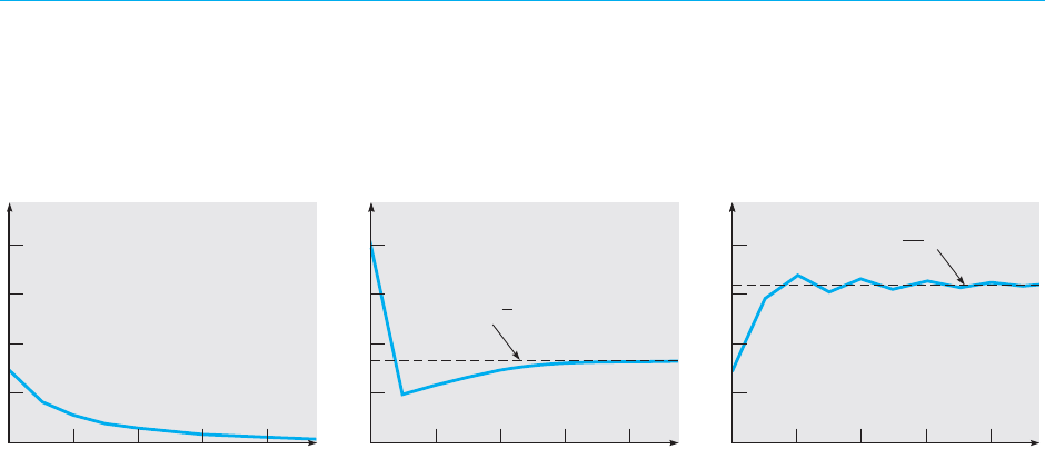
August 7, 2012 21:03 c02 Sheet number 97 Page number 127 cyan black
2.9 First Order Difference Equations 127
and to the nonzero equilibrium solution for ρ = 1.5 and ρ = 2.8. The convergence is
monotone for ρ = 0.8 and ρ = 1.5 and is oscillatory for ρ = 2.8. The graphs shown
are for particular initial conditions, but the graphs for other initial conditions are
similar.
2648
( a)
0.8
0.6
0.4
0.2
n
u
n
2648
( b)
0.8
0.6
0.4
0.2
n
u
n
u
n
=
1
3
2648
( c)
0.8
0.6
0.4
0.2
u
n
= = 0.6429
~
1.8
2.8
n
u
n
FIGURE 2.9.1 Solutions of u
n+1
= ρu
n
(1 − u
n
):(a) ρ = 0.8; (b) ρ = 1.5; (c) ρ = 2.8.
Another way of displaying the solution of a difference equation is shown in
Figure 2.9.2. In each part of this figure, the graphs of the parabola y = ρx(1 − x)
and of the straight line y = x are shown. The equilibrium solutions correspond to
the points of intersection of these two curves. The piecewise linear graph consist-
ing of successive vertical and horizontal line segments, sometimes called a stairstep
diagram, represents the solution sequence. The sequence starts at the point u
0
on
the x-axis. The vertical line segment drawn upward to the parabola at u
0
corresponds
to thecalculation of ρu
0
(1 − u
0
) = u
1
.This value isthen transferred from the y-axis to
the x-axis; this step is represented by the horizontal line segment from the parabola
to the line y = x. Then the process is repeated over and over again. Clearly, the
sequence converges to the origin in Figure 2.9.2a and to the nonzero equilibrium
solution in the other two cases.
To summarize our results so far: the difference equation (21) has two equilib-
rium solutions, u
n
= 0 and u
n
= (ρ − 1)/ρ; the former is asymptotically stable for
0 ≤ ρ<1, and the latter is asymptotically stable for 1 <ρ<3. When ρ = 1, the two
equilibrium solutions coincide at u = 0; this solution can be shown to be asymptoti-
cally stable. In Figure 2.9.3 the parameter ρ is plotted on the horizontal axis and u on
the vertical axis. The equilibrium solutions u = 0 and u = (ρ − 1)/ρ are shown. The
intervals in which each one is asymptotically stable are indicated by the solid portions
of the curves. There is an exchange of stability from one equilibrium solution to the
other at ρ = 1.
For ρ>3, neither of the equilibrium solutions is stable, and the solutions of
Eq. (21) exhibit increasing complexity as ρ increases. For ρ somewhat greater than 3,
the sequence u
n
rapidly approaches a steady oscillation of period 2; that is, u
n
oscil-
lates back and forth between two distinct values. For ρ = 3.2, a solution is shown in
Figure 2.9.4. For n greater than about 20, the solution alternates between the values
0.5130 and 0.7995. The graph is drawn for the particular initial condition u
0
= 0.3,
but it is similar for all other initial values between 0 and 1. Figure 2.9.4b also shows
the same steady oscillation as a rectangular path that is traversed repeatedly in the
clockwise direction.

August 7, 2012 21:03 c02 Sheet number 98 Page number 128 cyan black
128 Chapter 2. First Order Differential Equations
( a)
0.8
0.6
0.4
0.2
y
0.2 0.4 0.6 0.8 1
y = x
u
0
= 0.3
x
y = x (1 – x)
ρ
( b)
0.2 0.4 0.6 0.8 1
x
y = x
u
0
= 0.85
1
3
1
3
,
y = x (1 – x)
ρ
0.8
0.6
0.4
0.2
y
0.2 0.4 0.6 0.8
( c)
1
y = x
(0.6429..., 0.6429...)
y
1
x
u
0
= 0.3
y = x (1 – x)
ρ
0.8
0.6
0.4
0.2
FIGURE 2.9.2 Iterates of u
n+1
= ρu
n
(1 − u
n
):(a) ρ = 0.8; (b) ρ = 1.5; (c) ρ = 2.8.
1
0.5
–0.5
123
ρ
u
u = 0
Asymptotically stable
Unstable
u = ( – 1)/
ρρ
FIGURE 2.9.3 Exchange of stability for u
n+1
= ρu
n
(1 − u
n
).

August 7, 2012 21:03 c02 Sheet number 99 Page number 129 cyan black
2.9 First Order Difference Equations 129
0.8
0.6
0.4
0.2
10 20 30 40
n
u
n
(a)
0.7995
0.5130
0.8
1
0.6
0.4
0.2
0.2 0.4 0.6 0.8 1
y = x
0.5130 0.7995
0.5130
0.7995
(b)
x
y
y = x (1 – x)
ρ
FIGURE 2.9.4 A solution of u
n+1
= ρu
n
(1 − u
n
) for
ρ = 3.2; period 2. (a) u
n
versus n;(b) a two-cycle.
At about ρ = 3.449, each state in the oscillation of period 2 separates into two
distinct states,andthe solution becomes periodic with period 4;see Figure 2.9.5,which
shows a solution of period 4 for ρ = 3.5. As ρ increases further, periodic solutions
of period 8, 16, ... appear. The appearance of a new solution at a certain parameter
value is called a bifurcation.
The ρ-values at which the successive period doublings occur approach a limit that
is approximately 3.57. For ρ>3.57, the solutions possess some regularity but no
discernible detailed pattern for most values of ρ. For example,a solution for ρ = 3.65
is shown in Figure 2.9.6. It oscillates between approximately 0.3 and 0.9, but its fine
structure is unpredictable. The term chaotic is used to describe this situation. One of
the features of chaotic solutions is extreme sensitivity to the initial conditions. This
is illustrated in Figure 2.9.7, where two solutions of Eq. (21) for ρ = 3.65 are shown.
One solution is the same as that in Figure 2.9.6 and has the initial value u
0
= 0.3,while
the other solution has the initial value u
0
= 0.305. For about 15 iterations the two
solutions remain close and are hard to distinguish from each other in the figure. After
that,although they continue to wander about in approximately the same set of values,

August 7, 2012 21:03 c02 Sheet number 100 Page number 130 cyan black
130 Chapter 2. First Order Differential Equations
0.8
0.4
841216202428323640
n
(a)
u
n
y
x
0.5
0.5
ρ
y = x (1 – x)
1
1
y = x
0.5009
0.3828
0.8269
0.8750
(b)
FIGURE 2.9.5 A solution of u
n+1
= ρu
n
(1 − u
n
) for ρ = 3.5;
period 4. (a) u
n
versus n;(b) a four-cycle.
0.3
10 20 30 40 50 60
0.4
0.5
0.6
0.7
0.8
0.9
n
u
n
FIGURE 2.9.6 A solution of u
n+1
= ρu
n
(1 − u
n
) for ρ = 3.65; a chaotic solution.

August 7, 2012 21:03 c02 Sheet number 101 Page number 131 cyan black
2.9 First Order Difference Equations 131
0.8
0.9
0.7
0.6
0.3
0.4
0.5
10 20 30 40 50 60
n
u
n
FIGURE 2.9.7 Two solutions of u
n+1
= ρu
n
(1 − u
n
) for ρ = 3.65; u
0
= 0.3 and u
0
= 0.305.
their graphs are quite dissimilar. It would certainly not be possible to use one of these
solutions to estimate the value of the other for values of n larger than about 15.
It is only comparativelyrecently that chaoticsolutions ofdifference anddifferential
equations have become widely known. Equation (20) was one of the first instances of
mathematical chaos to be found and studied in detail, by Robert May
21
in 1974. On
the basis of his analysis of this equation as a model of the population of certain insect
species, May suggested that if the growth rate ρ is too large, then it will be impossible
to make effective long-range predictions about these insect populations. The occur-
rence of chaotic solutions in seemingly simple problems has stimulated an enormous
amount of research, but many questions remain unanswered. It is increasingly clear,
however, that chaotic solutions are much more common than was suspected at first
and that they may be a part of the investigation of a wide range of phenomena.
PROBLEMS In each of Problems 1 through 6, solve the given difference equation in terms of the initial
value y
0
. Describe the behavior of the solution as n →∞.
1. y
n+1
=−0.9y
n
2. y
n+1
=
n + 1
n + 2
y
n
3. y
n+1
=
:
n + 3
n + 1
y
n
4. y
n+1
= (−1)
n+1
y
n
5. y
n+1
= 0.5y
n
+ 66.y
n+1
=−0.5y
n
+ 6
21
Robert M. May (1938– ) was born in Sydney, Australia, and received his education at the University of
Sydney with a doctorate in theoretical physics in 1959. His interests soon turned to population dynamics
and theoretical ecology; the work cited in the text is described in two papers listed in the References at
the end of this chapter. He has held professorships at Sydney, at Princeton, at Imperial College (London),
and (since 1988) at Oxford.

August 7, 2012 21:03 c02 Sheet number 102 Page number 132 cyan black
132 Chapter 2. First Order Differential Equations
7. Find the effective annual yield of a bank account that pays interest at a rate of 7%,
compounded daily; that is, divide the difference between the final and initial balances by
the initial balance.
8. An investor deposits $1000 in an account paying interest at a rate of 8%, compounded
monthly, and also makes additional deposits of $25 per month. Find the balance in the
account after 3 years.
9. A certain college graduate borrows $8000 to buy a car. The lender charges interest at an
annual rate of 10%. What monthly payment rate is required to pay off the loan in 3 years?
Compare your result with that of Problem 9 in Section 2.3.
10. A homebuyer wishesto take outa mortgage of$100,000 for a30-year period.What monthly
payment is required if the interest rate is (a) 9%, (b) 10%, (c) 12%?
11. A homebuyer takes out a mortgage of $100,000 with an interest rate of 9%.What monthly
payment is required to pay off the loan in 30 years? In 20 years? What is the total amount
paid during the term of the loan in each of these cases?
12. If the interest rate on a 20-year mortgage is fixed at 10% and if a monthly payment of
$1000 is the maximum that the buyer can afford, what is the maximum mortgage loan that
can be made under these conditions?
13. A homebuyer wishes to finance the purchase with a $95,000 mortgage with a 20-year term.
What is the maximum interest rate the buyer can afford if the monthly payment is not to
exceed $900?
The Logistic Difference Equation. Problems 14 through 19 deal with the difference equation
(21), u
n+1
= ρu
n
(1 − u
n
).
14. Carry out the details in the linear stability analysis of the equilibrium solution
u
n
= (ρ − 1)/ρ. That is, derive the difference equation (26) in the text for the pertur-
bation v
n
.
15.
(a) For ρ = 3.2, plot or calculate the solution of the logistic equation (21) for several
initial conditions, say, u
0
= 0.2, 0.4, 0.6, and 0.8. Observe that in each case the solution
approaches a steady oscillation between the same two values. This illustrates that the
long-term behavior of the solution is independent of the initial conditions.
(b) Make similar calculations and verify that the nature of the solution for large n is
independent of the initial condition for other values of ρ, such as 2.6, 2.8, and 3.4.
16. Assume that ρ>1 in Eq. (21).
(a) Draw a qualitatively correct stairstep diagram and thereby show that if u
0
< 0, then
u
n
→−∞as n →∞.
(b) In a similar way, determine what happens as n →∞if u
0
> 1.
17.
The solutions of Eq. (21) change from convergent sequences to periodic oscillations of
period 2 as the parameter ρ passes through the value 3. To see more clearly how this
happens, carry out the following calculations.
(a) Plot or calculate the solution for ρ = 2.9, 2.95, and 2.99, respectively, using an initial
value u
0
of your choice in the interval (0, 1). In each case estimate how many iterations
are required for the solution to get “very close” to the limiting value. Use any convenient
interpretation of what “very close” means in the preceding sentence.
(b) Plot or calculate the solution for ρ = 3.01, 3.05, and 3.1, respectively, using the same
initial condition as in part (a). In each case estimate how many iterations are needed to
reach a steady-state oscillation. Also find or estimate the two values in the steady-state
oscillation.

August 7, 2012 21:03 c02 Sheet number 103 Page number 133 cyan black
2.9 First Order Difference Equations 133
18. By calculating or plotting the solution of Eq. (21) for different values of ρ, estimate the
value of ρ at which the solution changes from an oscillation of period 2 to one of period
4. In the same way, estimate the value of ρ at which the solution changes from period 4 to
period 8.
19.
Let ρ
k
be the value of ρ at which the solution of Eq. (21) changes from period 2
k−1
to
period 2
k
. Thus, as noted in the text, ρ
1
= 3, ρ
2
∼
=
3.449, and ρ
3
∼
=
3.544.
(a) Using these values of ρ
1
, ρ
2
, and ρ
3
, or those you found in Problem 18, calculate
(ρ
2
− ρ
1
)/(ρ
3
− ρ
2
).
(b) Letδ
n
= (ρ
n
− ρ
n−1
)/(ρ
n+1
− ρ
n
). It can beshown that δ
n
approachesa limit δ as n →∞,
where δ
∼
=
4.6692 is known as the Feigenbaum
22
number. Determine the percentage
difference between the limiting value δ and δ
2
, as calculated in part (a).
(c) Assume that δ
3
= δ and use this relation to estimate ρ
4
,the valueof ρ at whichsolutions
of period 16 appear.
(d) By plotting or calculating solutions near the value of ρ
4
found in part (c), try to detect
the appearance of a period 16 solution.
(e) Observe that
ρ
n
= ρ
1
+ (ρ
2
− ρ
1
) + (ρ
3
− ρ
2
) +···+(ρ
n
− ρ
n−1
).
Assuming that (ρ
4
− ρ
3
) = (ρ
3
− ρ
2
)δ
−1
, (ρ
5
− ρ
4
) = (ρ
3
− ρ
2
)δ
−2
, and so forth, express ρ
n
as a geometric sum. Then find the limit of ρ
n
as n →∞. This is an estimate of the value of
ρ at which the onset of chaos occurs in the solution of the logistic equation (21).
PROBLEMS Miscellaneous Problems. One of the difficulties in solving first order equations is that there
are several methods of solution, each of which can be used on a certain type of equation. It
may take some time to become proficient in matching solution methods with equations. The
first 32 of the following problems are presented to give you some practice in identifying the
method or methods applicable to a given equation. The remaining problems involve certain
types of equations that can be solved by specialized methods.
In each of Problems 1 through 32, solve the given differential equation. If an initial condition
is given, also find the solution that satisfies it.
1.
dy
dx
=
x
3
− 2y
x
2.
dy
dx
=
1 + cos x
2 − sin y
3.
dy
dx
=
2x + y
3 + 3y
2
− x
, y(0) = 04.
dy
dx
= 3 − 6x + y − 2xy
5.
dy
dx
=−
2xy + y
2
+ 1
x
2
+ 2xy
6. x
dy
dx
+ xy = 1 − y, y(1) = 0
7.
dy
dx
=
4x
3
+ 1
y(2 + 3y)
8. x
dy
dx
+ 2y =
sin x
x
, y(2) = 1
22
This result for the logistic difference equation was discovered in August 1975 by Mitchell Feigenbaum
(1944– ), while he was working at the LosAlamos National Laboratory. Within a few weeks he had estab-
lished that the same limiting value also appears in a large class of period-doubling difference equations.
Feigenbaum, who has a doctorate in physics from M.I.T., is now at Rockefeller University.

August 7, 2012 21:03 c02 Sheet number 104 Page number 134 cyan black
134 Chapter 2. First Order Differential Equations
9.
dy
dx
=−
2xy + 1
x
2
+ 2y
10. (x
2
y + xy − y) + (x
2
y − 2x
2
)
dy
dx
= 0
11. (x
2
+ y) + (x + e
y
)
dy
dx
= 0 12.
dy
dx
+ y =
1
1 + e
x
13.
dy
dx
= 1 + 2x + y
2
+ 2xy
2
14. (x + y) + (x + 2y)
dy
dx
= 0, y(2) = 3
15. (e
x
+ 1)
dy
dx
= y − ye
x
16.
dy
dx
=
e
−x
cos y − e
2y
cos x
−e
−x
sin y + 2e
2y
sin x
17.
dy
dx
= e
2x
+ 3y 18.
dy
dx
+ 2y = e
−x
2
−2x
, y(0) = 3
19.
dy
dx
=
3x
2
− 2y − y
3
2x + 3xy
2
20. y
′
= e
x+y
21.
dy
dx
+
2y
2
+ 6xy − 4
3x
2
+ 4xy + 3y
2
= 0 22.
dy
dx
=
x
2
− 1
y
2
+ 1
, y(−1) = 1
23. t
dy
dt
+ (t + 1)y = e
2t
24. 2 sin y sin x cos x + cos y sin
2
x
dy
dx
= 0
25.
'
2
x
y
−
y
x
2
+ y
2
(
+
'
x
x
2
+ y
2
−
x
2
y
2
(
dy
dx
= 0
26. xy
′
= y + xe
y/x
27.
dy
dx
=
x
x
2
y + y
3
Hint: Let u = x
2
.
28. (2y + 3x) =−x
dy
dx
29.
dy
dx
=
x + y
x − y
30. (3y
2
+ 2xy) − (2xy + x
2
)
dy
dx
= 0 31.
dy
dx
=−
3x
2
y + y
2
2x
3
+ 3xy
, y(1) =−2
32. xy
′
+ y − y
2
e
2x
= 0, y(1) = 2
33. Riccati Equations. The equation
dy
dt
= q
1
(t) + q
2
(t)y + q
3
(t)y
2
is known as a Riccati
23
equation. Suppose that some particular solution y
1
of this equation
is known. A more general solution containing one arbitrary constant can be obtained
through the substitution
y = y
1
(t) +
1
v(t)
.
Show that v(t) satisfies the first order linear equation
dv
dt
=−(q
2
+ 2q
3
y
1
)v − q
3
.
Note that v(t) will contain a single arbitrary constant.
23
Riccati equations are named for Jacopo Francesco Riccati (1676–1754), a Venetian nobleman, who
declined university appointments in Italy,Austria, and Russia to pursue his mathematical studies privately
at home. Riccati studied these equations extensively; however, it was Euler (in 1760) who discovered the
result stated in this problem.

August 7, 2012 21:03 c02 Sheet number 105 Page number 135 cyan black
2.9 First Order Difference Equations 135
34. Using the method of Problem 33 and the given particular solution, solve each of the
following Riccati equations:
(a) y
′
= 1 + t
2
− 2ty + y
2
; y
1
(t) = t (b) y
′
=−
1
t
2
−
y
t
+ y
2
; y
1
(t) =
1
t
(c)
dy
dt
=
2 cos
2
t − sin
2
t + y
2
2 cos t
; y
1
(t) = sin t
35. The propagation of a single action in a large population (for example, drivers turning on
headlights at sunset) often depends partly on external circumstances (gathering darkness)
and partly on a tendency to imitate others who have already performed the action in
question. In this case the proportion y(t) of people who have performed the action can be
described
24
by the equation
dy/dt = (1 − y)[x(t) + by], (i)
where x(t) measures the external stimulus and b is the imitation coefficient.
(a) Observe that Eq. (i) is a Riccati equation and that y
1
(t) = 1 is one solution. Use the
transformation suggested in Problem 33, and find the linear equation satisfied by v(t).
(b) Find v(t) in the case that x(t) = at, where a is a constant. Leave your answer in the
form of an integral.
Some Special Second Order Equations. Second order equations involve the second deriva-
tive of the unknown function and have the general form y
′′
= f (t, y, y
′
). Usually such equations
cannot be solved by methods designed for first order equations. However, there are two types
of second order equations that can be transformed into first order equations by a suitable
change of variable. The resulting equation can sometimes be solved by the methods presented
in this chapter. Problems 36 through 51 deal with these types of equations.
Equations with the Dependent Variable Missing. For a second order differential equation
of the form y
′′
= f (t, y
′
), the substitution v = y
′
, v
′
= y
′′
leads to a first order equation of the
form v
′
= f (t, v). If this equation can be solved for v, then y can be obtained by integrating
dy/dt = v. Note that one arbitrary constant is obtained in solving the first order equation for
v, and a second is introduced in the integration for y. In each of Problems 36 through 41, use
this substitution to solve the given equation.
36. t
2
y
′′
+ 2ty
′
− 1 = 0, t > 0 37. ty
′′
+ y
′
= 1, t > 0
38. y
′′
+ t(y
′
)
2
= 0 39. 2t
2
y
′′
+ (y
′
)
3
= 2ty
′
, t > 0
40. y
′′
+ y
′
= e
−t
41. t
2
y
′′
= (y
′
)
2
, t > 0
Equations with the Independent Variable Missing. Consider second order differential equa-
tions of the form y
′′
= f (y, y
′
), in which the independent variable t does not appear explicitly.
If we let v = y
′
,then we obtain dv/dt = f (y,v). Since the right side of this equation depends on
y and v, rather than on t and v,this equation contains too many variables. However, if we think
of y as the independent variable, then by the chain rule, dv/dt = (dv/dy)(dy/dt) = v(dv/dy).
Hence the original differential equation can be written as v(dv/dy) = f (y, v). Provided that
this first order equation can be solved, we obtain v as a function of y. A relation between y
and t results from solving dy/dt = v(y), which is a separable equation. Again, there are two
24
See Anatol Rapoport,“Contribution to the Mathematical Theory of Mass Behavior: I. The Propagation
of Single Acts,” Bulletin of Mathematical Biophysics 14 (1952), pp. 159–169, and John Z. Hearon, “Note
on the Theory of Mass Behavior,” Bulletin of Mathematical Biophysics 17 (1955), pp. 7–13.

August 7, 2012 21:03 c02 Sheet number 106 Page number 136 cyan black
136 Chapter 2. First Order Differential Equations
arbitrary constants in the final result. In each of Problems 42 through 47, use this method to
solve the given differential equation.
42. yy
′′
+ (y
′
)
2
= 0 43. y
′′
+ y = 0
44. y
′′
+ y(y
′
)
3
= 0 45. 2y
2
y
′′
+ 2y(y
′
)
2
= 1
46. yy
′′
− (y
′
)
3
= 0 47. y
′′
+ (y
′
)
2
= 2e
−y
Hint: In Problem 47 the transformed equation is a Bernoulli equation. See Problem 27 in
Section 2.4.
In each of Problems 48 through 51, solve the given initial value problem using the methods of
Problems 36 through 47.
48. y
′
y
′′
= 2, y(0) = 1, y
′
(0) = 2
49. y
′′
− 3y
2
= 0, y(0) = 2, y
′
(0) = 4
50. (1 + t
2
)y
′′
+ 2ty
′
+ 3t
−2
= 0, y(1) = 2, y
′
(1) =−1
51. y
′
y
′′
− t = 0, y(1) = 2, y
′
(1) = 1
REFERENCES The two books mentioned in Section 2.5 are
Bailey, N. T. J.,The Mathematical Theory of Infectious Diseases and Its Applications (2nd ed.) (New York:
Hafner Press, 1975).
Clark, Colin W., Mathematical Bioeconomics (2nd ed.) (New York: Wiley-Interscience, 1990).
A good introduction to population dynamics in general is
Frauenthal, J. C., Introduction to Population Modeling (Boston: Birkhauser, 1980).
A fuller discussion of the proof of the fundamental existence and uniqueness theorem can be found in
many more advanced books on differential equations. Two that are reasonably accessible to elementary
readers are
Coddington, E. A., An Introduction to Ordinary Differential Equations (Englewood Cliffs, NJ: Prentice-
Hall, 1961; New York: Dover, 1989).
Brauer,F.,and Nohel,J.,The Qualitative Theory of Ordinary Differential Equations (New York: Benjamin,
1969; New York: Dover, 1989).
A valuable compendium of methods for solving differential equations is
Zwillinger, D., Handbook of Differential Equations (3rd ed.) (San Diego:Academic Press, 1998).
For further discussion and examples of nonlinear phenomena, including bifurcations and chaos, see
Strogatz, Steven H., Nonlinear Dynamics and Chaos (Reading, MA:Addison-Wesley, 1994).
A general reference on difference equations is
Mickens, R. E., Difference Equations, Theory and Applications (2nd ed.) (New York: Van Nostrand
Reinhold, 1990).
Two papers by Robert May cited in the text are
R. M. May,“Biological Populations with Nonoverlapping Generations:Stable Points,Stable Cycles,and
Chaos,” Science 186 (1974), pp. 645–647; “Biological Populations Obeying Difference Equations: Stable
Points, Stable Cycles, and Chaos,” Journal of Theoretical Biology 51 (1975), pp. 511–524.
An elementary treatment of chaotic solutions of difference equations is
Devaney, R. L., Chaos, Fractals, and Dynamics (Reading, MA:Addison-Wesley, 1990).

August 7, 2012 21:04 c03 Sheet number 1 Page number 137 cyan black
137
CHAPTER
3
Second Order Linear
Equations
Linear equations of second order are of crucial importance in the study of differential
equations for two main reasons. The first is that linear equations have a rich theo-
retical structure that underlies a number of systematic methods of solution. Further,
a substantial portion of this structure and of these methods is understandable at a
fairly elementary mathematical level. In order to present the key ideas in the sim-
plest possible context, we describe them in this chapter for second order equations.
Another reason to study second order linear equations is that they are vital to any
serious investigation of the classical areas of mathematical physics. One cannot go
very far in the development of fluid mechanics, heat conduction, wave motion, or
electromagnetic phenomena without finding it necessary to solve second order lin-
ear differential equations. As an example, we discuss the oscillations of some basic
mechanical and electrical systems at the end of the chapter.
3.1 Homogeneous Equations with Constant Coefficients
A second order ordinary differential equation has the form
d
2
y
dt
2
= f
'
t, y,
dy
dt
(
, (1)
where f is some given function. Usually, we will denote the independent variable
by t since time is often the independent variable in physical problems, but some-
times we will use x instead. We will use y, or occasionally some other letter, to
designate the dependent variable. Equation (1) is said to be linear if the function f

August 7, 2012 21:04 c03 Sheet number 2 Page number 138 cyan black
138 Chapter 3. Second Order Linear Equations
has the form
f
'
t, y,
dy
dt
(
= g(t) − p(t)
dy
dt
− q(t)y, (2)
that is, if f is linear in y and dy/dt. In Eq. (2) g, p, and q are specified functions of
the independent variable t but do not depend on y. In this case we usually rewrite
Eq. (1) as
y
′′
+ p(t)y
′
+ q(t)y = g(t), (3)
where the primes denote differentiation with respect to t. Instead of Eq. (3),we often
see the equation
P(t)y
′′
+ Q(t)y
′
+ R(t)y = G(t). (4)
Of course, if P(t) ̸= 0, we can divide Eq. (4) by P(t) and thereby obtain Eq. (3) with
p(t) =
Q(t)
P(t)
, q(t) =
R(t)
P(t)
, g(t) =
G(t)
P(t)
. (5)
In discussing Eq. (3) and in trying to solve it, we will restrict ourselves to intervals in
which p, q, and g are continuous functions.
1
If Eq. (1) is not of the form (3) or (4), then it is called nonlinear. Analytical investi-
gations of nonlinear equationsare relativelydifficult,so we willhave littleto sayabout
them in this book. Numerical or geometical approaches are often more appropriate,
and these are discussed in Chapters 8 and 9.
An initial value problem consists of a differential equation such as Eq. (1), (3), or
(4) together with a pair of initial conditions
y(t
0
) = y
0
, y
′
(t
0
) = y
′
0
, (6)
where y
0
and y
′
0
are given numbers prescribing values for y and y
′
at the initial
point t
0
. Observe that the initial conditions for a second order equation identify not
only a particular point (t
0
, y
0
) through which the graph of the solution must pass,
but also the slope y
′
0
of the graph at that point. It is reasonable to expect that two
initial conditions are needed for a second order equation because, roughly speaking,
two integrations are required to find a solution and each integration introduces an
arbitrary constant. Presumably, two initial conditions will suffice to determine values
for these two constants.
A second order linear equation is said to be homogeneous if the term g(t) in
Eq. (3), or the term G(t) in Eq. (4), is zero for all t. Otherwise, the equation is
called nonhomogeneous. As a result, the term g(t),orG(t), is sometimes called the
nonhomogeneous term.We beginour discussion with homogeneous equations,which
we will write in the form
P(t)y
′′
+ Q(t)y
′
+ R(t)y = 0. (7)
Later, in Sections 3.5 and 3.6, we will show that once the homogeneous equation
has been solved, it is always possible to solve the corresponding nonhomogeneous
1
There is a corresponding treatment of higher order linear equations in Chapter 4. If you wish, you may
read the appropriate parts of Chapter 4 in parallel with Chapter 3.

August 7, 2012 21:04 c03 Sheet number 3 Page number 139 cyan black
3.1 Homogeneous Equations with Constant Coefficients 139
equation (4), or at least to express the solution in terms of an integral. Thus the
problem of solving the homogeneous equation is the more fundamental one.
In this chapter we will concentrate our attention on equations in which the
functions P, Q, and R are constants. In this case, Eq. (7) becomes
ay
′′
+ by
′
+ cy = 0, (8)
where a, b, and c are given constants. It turns out that Eq. (8) can always be solved
easily in terms of the elementary functions of calculus. On the other hand, it is usu-
ally much more difficult to solve Eq. (7) if the coefficients are not constants, and
a treatment of that case is deferred until Chapter 5. Before taking up Eq. (8), let
us first gain some experience by looking at a simple example that in many ways is
typical.
EXAMPLE
1
Solve the equation
y
′′
− y = 0, (9)
and also find the solution that satisfies the initial conditions
y(0) = 2, y
′
(0) =−1. (10)
Observe that Eq. (9) is just Eq. (8) with a = 1, b = 0, and c =−1. In words, Eq. (9) says that
we seek a function with the property that the second derivative of the function is the same as the
function itself. Do any of the functions that you studied in calculus have this property? A little
thought will probably produce at least one such function, namely, y
1
(t) = e
t
, the exponential
function. A little more thought may also produce a second function, y
2
(t) = e
−t
. Some further
experimentation reveals that constant multiples of these two solutions are also solutions. For
example, the functions 2e
t
and 5e
−t
also satisfy Eq. (9), as you can verify by calculating their
second derivatives. In the same way, the functions c
1
y
1
(t) = c
1
e
t
and c
2
y
2
(t) = c
2
e
−t
satisfy the
differential equation (9) for all values of the constants c
1
and c
2
.
Next, it is vital to notice that the sum of any two solutions of Eq. (9) is also a solution.
In particular, since c
1
y
1
(t) and c
2
y
2
(t) are solutions of Eq. (9) for any values of c
1
and c
2
, so is
the function
y = c
1
y
1
(t) + c
2
y
2
(t) = c
1
e
t
+ c
2
e
−t
. (11)
Again, this can be verified by calculating the second derivative y
′′
from Eq. (11). We have
y
′
= c
1
e
t
− c
2
e
−t
and y
′′
= c
1
e
t
+ c
2
e
−t
; thus y
′′
is the same as y, and Eq. (9) is satisfied.
Letus summarize what we havedone so far in thisexample.Oncewe notice that the functions
y
1
(t) = e
t
and y
2
(t) = e
−t
are solutions of Eq. (9),it follows that the general linear combination
(11) of these functions is also a solution. Since the coefficients c
1
and c
2
in Eq. (11) are arbitrary,
this expression represents an infinite family of solutions of the differential equation (9).
It is now possible to consider how to pick out a particular member of this infinite family of
solutions that also satisfies a given set of initial conditions (10). In other words, we seek the
solution that passes through the point (0, 2) and at that point has the slope −1. First, we set
t = 0 and y = 2 in Eq. (11); this gives the equation
c
1
+ c
2
= 2. (12)
Next, we differentiate Eq. (11) with the result that
y
′
= c
1
e
t
− c
2
e
−t
.

August 7, 2012 21:04 c03 Sheet number 4 Page number 140 cyan black
140 Chapter 3. Second Order Linear Equations
Then, setting t = 0 and y
′
=−1, we obtain
c
1
− c
2
=−1. (13)
By solving Eqs. (12) and (13) simultaneously for c
1
and c
2
, we find that
c
1
=
1
2
, c
2
=
3
2
. (14)
Finally, inserting these values in Eq. (11), we obtain
y =
1
2
e
t
+
3
2
e
−t
, (15)
the solution of the initial value problem consisting of the differential equation (9) and the
initial conditions (10).
What conclusions can we draw from the preceding example that will help us to
deal with the more general equation (8),
ay
′′
+ by
′
+ cy = 0,
whose coefficients a, b, and c are arbitrary (real) constants? In the first place, in the
example the solutions were exponential functions. Further, once we had identified
two solutions, we were able to use a linear combination of them to satisfy the given
initial conditions as well as the differential equation itself.
It turns out that by exploiting these two ideas, we can solve Eq. (8) for any values
of its coefficients and also satisfy any given set of initial conditions for y and y
′
.
We start by seeking exponential solutions of the form y = e
rt
, where r is a parameter
to be determined. Then it follows that y
′
= re
rt
and y
′′
= r
2
e
rt
. By substituting these
expressions for y, y
′
, and y
′′
in Eq. (8), we obtain
(ar
2
+ br + c)e
rt
= 0,
or, since e
rt
̸= 0,
ar
2
+ br + c = 0. (16)
Equation (16) is called the characteristic equation for the differential equation (8).
Its significance lies in the fact that if r is a root of the polynomial equation (16), then
y = e
rt
is a solution of the differential equation (8). Since Eq. (16) is a quadratic
equation with real coefficients, it has two roots, which may be real and different, real
but repeated, or complex conjugates. We consider the first case here and the latter
two cases in Sections 3.3 and 3.4.
Assuming that the roots of the characteristic equation (16) are real and different,
let them be denoted by r
1
and r
2
, where r
1
̸= r
2
. Then y
1
(t) = e
r
1
t
and y
2
(t) = e
r
2
t
are
two solutions of Eq. (8). Just as in Example 1, it now follows that
y = c
1
y
1
(t) + c
2
y
2
(t) = c
1
e
r
1
t
+ c
2
e
r
2
t
(17)
is also a solution of Eq. (8).To verify that this is so,we can differentiate the expression
in Eq. (17); hence
y
′
= c
1
r
1
e
r
1
t
+ c
2
r
2
e
r
2
t
(18)
and
y
′′
= c
1
r
2
1
e
r
1
t
+ c
2
r
2
2
e
r
2
t
. (19)

August 7, 2012 21:04 c03 Sheet number 5 Page number 141 cyan black
3.1 Homogeneous Equations with Constant Coefficients 141
Substituting these expressions for y, y
′
, and y
′′
in Eq. (8) and rearranging terms, we
obtain
ay
′′
+ by
′
+ cy = c
1
(ar
2
1
+ br
1
+ c)e
r
1
t
+ c
2
(ar
2
2
+ br
2
+ c)e
r
2
t
. (20)
The quantities in the two sets of parentheses on the right-hand side of Eq. (20) are
zero because r
1
and r
2
are roots of Eq. (16);therefore, y as given by Eq. (17) is indeed
a solution of Eq. (8), as we wished to verify.
Now suppose that we want to find the particular member of the family of solutions
(17) that satisfies the initial conditions (6)
y(t
0
) = y
0
, y
′
(t
0
) = y
′
0
.
By substituting t = t
0
and y = y
0
in Eq. (17), we obtain
c
1
e
r
1
t
0
+ c
2
e
r
2
t
0
= y
0
. (21)
Similarly, setting t = t
0
and y
′
= y
′
0
in Eq. (18) gives
c
1
r
1
e
r
1
t
0
+ c
2
r
2
e
r
2
t
0
= y
′
0
. (22)
On solving Eqs. (21) and (22) simultaneously for c
1
and c
2
, we find that
c
1
=
y
′
0
− y
0
r
2
r
1
− r
2
e
−r
1
t
0
, c
2
=
y
0
r
1
− y
′
0
r
1
− r
2
e
−r
2
t
0
. (23)
Recall that r
1
− r
2
̸= 0 so that the expressions in Eq. (23) always make sense. Thus,
no matter what initial conditions are assigned—that is, regardless of the values of
t
0
, y
0
, and y
′
0
in Eqs. (6)—it is always possible to determine c
1
and c
2
so that the
initial conditions are satisfied. Moreover, there is only one possible choice of c
1
and
c
2
for each set of initial conditions. With the values of c
1
and c
2
given by Eq. (23), the
expression (17) is the solution of the initial value problem
ay
′′
+ by
′
+ cy = 0, y(t
0
) = y
0
, y
′
(t
0
) = y
′
0
. (24)
It is possible to show, on the basis of the fundamental theorem cited in the next
section,that all solutions of Eq. (8) are included in the expression (17),at least for the
case in which the roots of Eq. (16) are real and different. Therefore, we call Eq. (17)
the general solution of Eq. (8). The fact that any possible initial conditions can be
satisfied by the proper choice of the constants in Eq. (17) makes more plausible the
idea that this expression does include all solutions of Eq. (8).
Let us now look at some further examples.
EXAMPLE
2
Find the general solution of
y
′′
+ 5y
′
+ 6y = 0. (25)
We assume that y = e
rt
, and it then followsthat r must bea root ofthe characteristicequation
r
2
+ 5r + 6 = (r + 2)(r + 3) = 0.
Thus the possible values of r are r
1
=−2 and r
2
=−3; the general solution of Eq. (25) is
y = c
1
e
−2t
+ c
2
e
−3t
. (26)

August 7, 2012 21:04 c03 Sheet number 6 Page number 142 cyan black
142 Chapter 3. Second Order Linear Equations
EXAMPLE
3
Find the solution of the initial value problem
y
′′
+ 5y
′
+ 6y = 0, y(0) = 2, y
′
(0) = 3. (27)
The general solution of the differential equation was found in Example 2 and is given by
Eq. (26). To satisfy the first initial condition, we set t = 0 and y = 2 in Eq. (26); thus c
1
and c
2
must satisfy
c
1
+ c
2
= 2. (28)
To use the second initial condition, we must first differentiate Eq. (26). This gives
y
′
=−2c
1
e
−2t
− 3c
2
e
−3t
. Then, setting t = 0 and y
′
= 3, we obtain
−2c
1
− 3c
2
= 3. (29)
By solving Eqs. (28) and (29), we find that c
1
= 9 and c
2
=−7. Using these values in the
expression (26), we obtain the solution
y = 9e
−2t
− 7e
−3t
(30)
of the initial value problem (27). The graph of the solution is shown in Figure 3.1.1.
y
t
2
1
0.5 1 1.5 2
y = 9e
–2t
– 7e
–3t
FIGURE 3.1.1 Solution of the initial value problem (27):
y
′′
+ 5y
′
+ 6y = 0, y(0) = 2, y
′
(0) = 3.
EXAMPLE
4
Find the solution of the initial value problem
4y
′′
− 8y
′
+ 3y = 0, y(0) = 2, y
′
(0) =
1
2
. (31)
If y = e
rt
, then we obtain the characteristic equation
4r
2
− 8r + 3 = 0
whose roots are r = 3/2 and r = 1/2. Therefore, the general solution of the differential
equation is
y = c
1
e
3t/2
+ c
2
e
t/2
. (32)
Applying the initial conditions, we obtain the following two equations for c
1
and c
2
:
c
1
+ c
2
= 2,
3
2
c
1
+
1
2
c
2
=
1
2
.
The solution of these equations is c
1
=−
1
2
, c
2
=
5
2
, so the solution of the initial value problem
(31) is
y =−
1
2
e
3t/2
+
5
2
e
t/2
. (33)
Figure 3.1.2 shows the graph of the solution.

August 7, 2012 21:04 c03 Sheet number 7 Page number 143 cyan black
3.1 Homogeneous Equations with Constant Coefficients 143
2
1
–1
0.5 1 1.5 2
y = – e
3t/2
+ e
t/2
1
2
5
2
y
t
FIGURE 3.1.2 Solution of the initial value problem (31):
4y
′′
− 8y
′
+ 3y = 0, y(0) = 2, y
′
(0) = 0.5.
EXAMPLE
5
The solution (30) of the initial value problem (27) initially increases (because its initial slope
is positive) but eventually approaches zero (because both terms involve negative exponential
functions). Therefore, the solution must have a maximum point, and the graph in Figure 3.1.1
confirms this. Determine the location of this maximum point.
The coordinates of the maximum point can be estimated from the graph, but to find
them more precisely, we seek the point where the solution has a horizontal tangent line.
By differentiating the solution (30), y = 9e
−2t
− 7e
−3t
, with respect to t, we obtain
y
′
=−18e
−2t
+ 21e
−3t
. (34)
Setting y
′
equal to zero and multiplying by e
3t
,we find that the critical value t
m
satisfies e
t
= 7/6;
hence
t
m
= ln(7/6)
∼
=
0.15415. (35)
The corresponding maximum value y
m
is given by
y
m
= 9e
−2t
m
− 7e
−3t
m
=
108
49
∼
=
2.20408. (36)
In this example the initial slope is 3, but the solution of the given differential equation
behaves in a similar way for any other positive initial slope. In Problem 26 you are asked to
determine how the coordinates of the maximum point depend on the initial slope.
Returning to the equation ay
′′
+ by
′
+ cy = 0 with arbitrary coefficients, recall
that when r
1
̸= r
2
, its general solution (17) is the sum of two exponential functions.
Therefore, the solution has a relatively simple geometrical behavior: as t increases,
the magnitude of the solution either tends to zero (when both exponents are nega-
tive) or else grows rapidly (when at least one exponent is positive). These two cases
are illustrated by the solutions of Examples 3 and 4, which are shown in Figures 3.1.1
and 3.1.2, respectively. There is also a third case that occurs less often: the solution
approaches a constant when one exponent is zero and the other is negative.
In Sections 3.3 and 3.4, respectively, we return to the problem of solving the
equation ay
′′
+ by
′
+ cy = 0 when the roots of the characteristic equation either
are complex conjugates or are real and equal. In the meantime, in Section 3.2,
we provide a systematic discussion of the mathematical structure of the solutions
of all second order linear homogeneous equations.

August 7, 2012 21:04 c03 Sheet number 8 Page number 144 cyan black
144 Chapter 3. Second Order Linear Equations
PROBLEMS In each of Problems 1 through 8, find the general solution of the given differential equation.
1. y
′′
+ 2y
′
− 3y = 02.y
′′
+ 3y
′
+ 2y = 0
3. 6y
′′
− y
′
− y = 04.2y
′′
− 3y
′
+ y = 0
5. y
′′
+ 5y
′
= 06.4y
′′
− 9y = 0
7. y
′′
− 9y
′
+ 9y = 08.y
′′
− 2y
′
− 2y = 0
In each of Problems 9 through 16, find the solution of the given initial value problem. Sketch
the graph of the solution and describe its behavior as t increases.
9. y
′′
+ y
′
− 2y = 0, y(0) = 1, y
′
(0) = 1
10. y
′′
+ 4y
′
+ 3y = 0, y(0) = 2, y
′
(0) =−1
11. 6y
′′
− 5y
′
+ y = 0, y(0) = 4, y
′
(0) = 0
12. y
′′
+ 3y
′
= 0, y(0) =−2, y
′
(0) = 3
13. y
′′
+ 5y
′
+ 3y = 0, y(0) = 1, y
′
(0) = 0
14. 2y
′′
+ y
′
− 4y = 0, y(0) = 0, y
′
(0) = 1
15. y
′′
+ 8y
′
− 9y = 0, y(1) = 1, y
′
(1) = 0
16. 4y
′′
− y = 0, y(−2) = 1, y
′
(−2) =−1
17. Find a differential equation whose general solution is y = c
1
e
2t
+ c
2
e
−3t
.
18. Find a differential equation whose general solution is y = c
1
e
−t/2
+ c
2
e
−2t
.
19.
Find the solution of the initial value problem
y
′′
− y = 0, y(0) =
5
4
, y
′
(0) =−
3
4
.
Plot the solution for 0 ≤ t ≤ 2 and determine its minimum value.
20. Find the solution of the initial value problem
2y
′′
− 3y
′
+ y = 0, y(0) = 2, y
′
(0) =
1
2
.
Then determine the maximum value of the solution and also find the point where the
solution is zero.
21. Solve the initial value problem y
′′
− y
′
− 2y = 0, y(0) = α, y
′
(0) = 2. Then find α so that
the solution approaches zero as t →∞.
22. Solve the initial value problem 4y
′′
− y = 0, y(0) = 2, y
′
(0) = β. Then find β so that the
solution approaches zero as t →∞.
In each of Problems 23 and 24, determine the values of α, if any, for which all solutions tend to
zero as t →∞; also determine the values of α,if any, for which all (nonzero) solutions become
unbounded as t →∞.
23. y
′′
− (2α − 1)y
′
+ α(α − 1)y = 0
24. y
′′
+ (3 − α)y
′
− 2(α − 1)y = 0
25.
Consider the initial value problem
2y
′′
+ 3y
′
− 2y = 0, y(0) = 1, y
′
(0) =−β,
where β>0.
(a) Solve the initial value problem.
(b) Plot the solution when β = 1. Find the coordinates (t
0
, y
0
) of the minimum point of
the solution in this case.
(c) Find the smallest value of β for which the solution has no minimum point.

August 7, 2012 21:04 c03 Sheet number 9 Page number 145 cyan black
3.2 Solutions of Linear Homogeneous Equations; the Wronskian 145
26. Consider the initial value problem (see Example 5)
y
′′
+ 5y
′
+ 6y = 0, y(0) = 2, y
′
(0) = β,
where β>0.
(a) Solve the initial value problem.
(b) Determine the coordinates t
m
and y
m
of the maximum point of the solution as func-
tions of β.
(c) Determine the smallest value of β for which y
m
≥ 4.
(d) Determine the behavior of t
m
and y
m
as β →∞.
27. Consider the equation ay
′′
+ by
′
+ cy = d, where a, b, c, and d are constants.
(a) Find all equilibrium, or constant, solutions of this differential equation.
(b) Let y
e
denote an equilibrium solution, and let Y = y − y
e
. Thus Y is the deviation of
a solution y from an equilibrium solution. Find the differential equation satisfied by Y.
28. Consider the equation ay
′′
+ by
′
+ cy = 0, where a, b, and c are constants with a > 0. Find
conditions on a, b, and c such that the roots of the characteristic equation are:
(a) real, different, and negative.
(b) real with opposite signs.
(c) real, different, and positive.
3.2 Solutions of Linear Homogeneous Equations; the Wronskian
In the preceding section we showed how to solve some differential equations of the
form
ay
′′
+ by
′
+ cy = 0,
where a, b, and c are constants. Now we build on those results to provide a clearer
picture of the structure of the solutions of all second order linear homogeneous
equations. In turn, this understanding will assist us in finding the solutions of other
problems that we will encounter later.
To discuss general properties of linear differential equations, it is helpful to intro-
duce a differential operator notation. Let p and q be continuous functions on an
open interval I—that is, for α<t <β. The cases for α =−∞,orβ =∞, or both,
are included. Then, for any function φ that is twice differentiable on I, we define the
differential operator L by the equation
L[φ]=φ
′′
+ pφ
′
+ qφ. (1)
Note that L[φ] is a function on I. The value of L[φ] at a point t is
L[φ](t) = φ
′′
(t) + p(t)φ
′
(t) + q(t)φ(t).
For example, if p(t) = t
2
, q(t) = 1 + t, and φ(t) = sin 3t, then
L[φ](t) = (sin 3t)
′′
+ t
2
(sin 3t)
′
+ (1 + t) sin 3t
=−9 sin 3t + 3t
2
cos 3t + (1 + t) sin 3t.

August 7, 2012 21:04 c03 Sheet number 10 Page number 146 cyan black
146 Chapter 3. Second Order Linear Equations
The operator L is often written as L = D
2
+ pD + q, where D is the derivative
operator.
In this section we study the second order linear homogeneous equation
L[φ](t) = 0. Since it is customary to use the symbol y to denote φ(t), we will usually
write this equation in the form
L[y]=y
′′
+ p(t)y
′
+ q(t)y = 0. (2)
With Eq. (2) we associate a set of initial conditions
y(t
0
) = y
0
, y
′
(t
0
) = y
′
0
, (3)
where t
0
is any point in the interval I, and y
0
and y
′
0
are given real numbers.
We would like to know whether the initial value problem (2), (3) always has a solu-
tion, and whether it may have more than one solution. We would also like to know
whether anything can be said about the form and structure of solutions that might
be helpful in finding solutions of particular problems. Answers to these questions are
contained in the theorems in this section.
The fundamental theoretical result for initial value problems for second order
linear equations is stated in Theorem 3.2.1, which is analogous to Theorem 2.4.1
for first order linear equations. The result applies equally well to nonhomogeneous
equations, so the theorem is stated in that form.
Theorem 3.2.1
(Existence and Uniqueness Theorem)
Consider the initial value problem
y
′′
+ p(t)y
′
+ q(t)y = g(t), y(t
0
) = y
0
, y
′
(t
0
) = y
′
0
, (4)
where p, q, and g are continuous on an open interval I that contains the point t
0
.
Then there is exactly one solution y = φ(t) of this problem, and the solution exists
throughout the interval I.
We emphasize that the theorem says three things:
1. The initial value problem has a solution; in other words, a solution exists.
2. The initial value problem has only one solution; that is, the solution is unique.
3. The solution φ is defined throughout the interval I where the coefficients are continuous
and is at least twice differentiable there.
For some problems some of these assertions are easy to prove. For instance, we
found in Example 1 of Section 3.1 that the initial value problem
y
′′
− y = 0, y(0) = 2, y
′
(0) =−1 (5)
has the solution
y =
1
2
e
t
+
3
2
e
−t
. (6)
The fact that we found a solution certainly establishes that a solution exists for this
initial value problem. Further,the solution (6) is twice differentiable,indeed differen-
tiable any number of times, throughout the interval (−∞, ∞) where the coefficients
in the differential equation are continuous. On the other hand, it is not obvious, and
is more difficult to show, that the initial value problem (5) has no solutions other

August 7, 2012 21:04 c03 Sheet number 11 Page number 147 cyan black
3.2 Solutions of Linear Homogeneous Equations; the Wronskian 147
than the one given by Eq. (6). Nevertheless, Theorem 3.2.1 states that this solution
is indeed the only solution of the initial value problem (5).
For most problems of the form (4), it is not possible to write down a useful expres-
sion for the solution. This is a major difference between first order and second order
linear equations.Therefore,all parts of the theorem must be proved by general meth-
ods that do not involve having such an expression.The proof ofTheorem 3.2.1 is fairly
difficult, and we do not discuss it here.
2
We will, however, accept Theorem 3.2.1 as
true and make use of it whenever necessary.
EXAMPLE
1
Find the longest interval in which the solution of the initial value problem
(t
2
− 3t)y
′′
+ ty
′
− (t + 3)y = 0, y(1) = 2, y
′
(1) = 1
is certain to exist.
If the given differential equation is written in the form of Eq. (4), then p(t) = 1/(t − 3),
q(t) =−(t + 3)/t(t − 3), and g(t) = 0. The only points of discontinuity of the coefficients are
t = 0 and t = 3. Therefore, the longest open interval, containing the initial point t = 1, in
which all the coefficients are continuous is 0 < t < 3. Thus, this is the longest interval in which
Theorem 3.2.1 guarantees that the solution exists.
EXAMPLE
2
Find the unique solution of the initial value problem
y
′′
+ p(t)y
′
+ q(t)y = 0, y(t
0
) = 0, y
′
(t
0
) = 0,
where p and q are continuous in an open interval I containing t
0
.
The function y = φ(t) = 0 for all t in I certainly satisfies the differential equation and ini-
tial conditions. By the uniqueness part of Theorem 3.2.1, it is the only solution of the given
problem.
Let us now assume that y
1
and y
2
are two solutions of Eq. (2); in other words,
L[y
1
]=y
′′
1
+ py
′
1
+ qy
1
= 0,
and similarly for y
2
. Then, just as in the examples in Section 3.1, we can generate
more solutions by forming linear combinations of y
1
and y
2
. We state this result as a
theorem.
Theorem 3.2.2
(Principle of Superposition)
If y
1
and y
2
are two solutions of the differential equation (2),
L[y]=y
′′
+ p(t)y
′
+ q(t)y = 0,
then the linear combination c
1
y
1
+ c
2
y
2
is also a solution for any values of the
constants c
1
and c
2
.
2
A proof of Theorem 3.2.1 can be found, for example, in Chapter 6, Section 8 of the book by Coddington
listed in the references at the end of this chapter.

August 7, 2012 21:04 c03 Sheet number 12 Page number 148 cyan black
148 Chapter 3. Second Order Linear Equations
A special case of Theorem 3.2.2 occurs if either c
1
or c
2
is zero. Then we conclude
that any constant multiple of a solution of Eq. (2) is also a solution.
To prove Theorem 3.2.2, we need only substitute
y = c
1
y
1
(t) + c
2
y
2
(t) (7)
for y in Eq. (2). By calculating the indicated derivatives and rearranging terms, we
obtain
L[c
1
y
1
+ c
2
y
2
]=[c
1
y
1
+ c
2
y
2
]
′′
+ p[c
1
y
1
+ c
2
y
2
]
′
+ q[c
1
y
1
+ c
2
y
2
]
= c
1
y
′′
1
+ c
2
y
′′
2
+ c
1
py
′
1
+ c
2
py
′
2
+ c
1
qy
1
+ c
2
qy
2
= c
1
[y
′′
1
+ py
′
1
+ qy
1
]+c
2
[y
′′
2
+ py
′
2
+ qy
2
]
= c
1
L[y
1
]+c
2
L[y
2
].
Since L[y
1
]=0 and L[y
2
]=0, it follows that L[c
1
y
1
+ c
2
y
2
]=0 also. Therefore,
regardless of the values of c
1
and c
2
, y as given by Eq. (7) satisfies the differential
equation (2), and the proof of Theorem 3.2.2 is complete.
Theorem 3.2.2 states that, beginning with only two solutions of Eq. (2), we can
construct an infinite family of solutions by means of Eq. (7). The next question is
whether all solutions of Eq. (2) are included in Eq. (7) or whether there may be
other solutions of a different form. We begin to address this question by examining
whether the constants c
1
and c
2
in Eq. (7) can be chosen so as to satisfy the initial
conditions (3). These initial conditions require c
1
and c
2
to satisfy the equations
c
1
y
1
(t
0
) + c
2
y
2
(t
0
) = y
0
,
(8)
c
1
y
′
1
(t
0
) + c
2
y
′
2
(t
0
) = y
′
0
.
The determinant of coefficients of the system (8) is
W =
3
3
3
3
3
y
1
(t
0
) y
2
(t
0
)
y
′
1
(t
0
) y
′
2
(t
0
)
3
3
3
3
3
= y
1
(t
0
)y
′
2
(t
0
) − y
′
1
(t
0
)y
2
(t
0
). (9)
If W ̸= 0, then Eqs. (8) have a unique solution (c
1
, c
2
) regardless of the values of
y
0
and y
′
0
. This solution is given by
c
1
=
y
0
y
′
2
(t
0
) − y
′
0
y
2
(t
0
)
y
1
(t
0
)y
′
2
(t
0
) − y
′
1
(t
0
)y
2
(t
0
)
, c
2
=
−y
0
y
′
1
(t
0
) + y
′
0
y
1
(t
0
)
y
1
(t
0
)y
′
2
(t
0
) − y
′
1
(t
0
)y
2
(t
0
)
, (10)
or, in terms of determinants,
c
1
=
3
3
3
3
3
y
0
y
2
(t
0
)
y
′
0
y
′
2
(t
0
)
3
3
3
3
3
3
3
3
3
3
y
1
(t
0
) y
2
(t
0
)
y
′
1
(t
0
) y
′
2
(t
0
)
3
3
3
3
3
, c
2
=
3
3
3
3
3
y
1
(t
0
) y
0
y
′
1
(t
0
) y
′
0
3
3
3
3
3
3
3
3
3
3
y
1
(t
0
) y
2
(t
0
)
y
′
1
(t
0
) y
′
2
(t
0
)
3
3
3
3
3
. (11)
With these values for c
1
and c
2
, the linear combination y = c
1
y
1
(t) + c
2
y
2
(t) satis-
fies the initial conditions (3) as well as the differential equation (2). Note that the
denominator in the expressions for c
1
and c
2
is the nonzero determinant W.
On the other hand, if W = 0, then the denominators appearing in Eqs. (10) and
(11) are zero. In this case Eqs. (8) have no solution unless y
0
and y
′
0
have values that
also make the numerators in Eqs. (10) and (11) equal to zero.Thus,if W = 0,there are
many initial conditions that cannot be satisfied no matter how c
1
and c
2
are chosen.

August 7, 2012 21:04 c03 Sheet number 13 Page number 149 cyan black
3.2 Solutions of Linear Homogeneous Equations; the Wronskian 149
The determinantW iscalledtheWronskian
3
determinant,orsimply theWronskian,
of the solutionsy
1
and y
2
. Sometimes weuse themore extended notationW(y
1
, y
2
)(t
0
)
to stand for the expression on the right side of Eq. (9), thereby emphasizing that the
Wronskian depends on the functions y
1
and y
2
, and that it is evaluated at the point
t
0
. The preceding argument establishes the following result.
Theorem 3.2.3
Suppose that y
1
and y
2
are two solutions of Eq. (2)
L[y]=y
′′
+ p(t)y
′
+ q(t)y = 0,
and that the initial conditions (3)
y(t
0
) = y
0
, y
′
(t
0
) = y
′
0
are assigned. Then it is always possible to choose the constants c
1
, c
2
so that
y = c
1
y
1
(t) + c
2
y
2
(t)
satisfies the differential equation (2) and the initial conditions (3) if and only if the
Wronskian
W = y
1
y
′
2
− y
′
1
y
2
is not zero at t
0
.
EXAMPLE
3
In Example 2 of Section 3.1 we found that y
1
(t) = e
−2t
and y
2
(t) = e
−3t
are solutions of the
differential equation
y
′′
+ 5y
′
+ 6y = 0.
Find the Wronskian of y
1
and y
2
.
The Wronskian of these two functions is
W =
3
3
3
3
e
−2t
e
−3t
−2e
−2t
−3e
−3t
3
3
3
3
=−e
−5t
.
Since W is nonzero for all values of t, the functions y
1
and y
2
can be used to construct solutions
of the given differential equation, together with initial conditions prescribed at any value of t.
One such initial value problem was solved in Example 3 of Section 3.1.
The next theorem justifies the term “general solution” that we introduced in
Section 3.1 for the linear combination c
1
y
1
+ c
2
y
2
.
Theorem 3.2.4
Suppose that y
1
and y
2
are two solutions of the differential equation (2),
L[y]=y
′′
+ p(t)y
′
+ q(t)y = 0.
Then the family of solutions
y = c
1
y
1
(t) + c
2
y
2
(t)
with arbitrary coefficients c
1
and c
2
includes every solution of Eq. (2) if and only if
there is a point t
0
where the Wronskian of y
1
and y
2
is not zero.
3
Wronskian determinants are named for Jósef Maria Hoëné-Wronski (1776–1853), who was born in Pol-
and but spent most of his life in France. Wronski was a gifted but troubled man, and his life was marked
by frequent heated disputes with other individuals and institutions.

August 7, 2012 21:04 c03 Sheet number 14 Page number 150 cyan black
150 Chapter 3. Second Order Linear Equations
Let φ be any solution of Eq. (2).To prove the theorem, we must determine whether
φ is included in the linear combinations c
1
y
1
+ c
2
y
2
. That is, we must determine
whether there are values of the constants c
1
and c
2
that make the linear combi-
nation the same as φ. Let t
0
be a point where the Wronskian of y
1
and y
2
is nonzero.
Then evaluate φ and φ
′
at this point and call these values y
0
and y
′
0
, respectively; thus
y
0
= φ(t
0
), y
′
0
= φ
′
(t
0
).
Next, consider the initial value problem
y
′′
+ p(t)y
′
+ q(t)y = 0, y(t
0
) = y
0
, y
′
(t
0
) = y
′
0
. (12)
The function φ is certainly a solution of this initial value problem. Further, because
we are assuming that W(y
1
, y
2
)(t
0
) is nonzero, it is possible (by Theorem 3.2.3)
to choose c
1
and c
2
such that y = c
1
y
1
(t) + c
2
y
2
(t) is also a solution of the initial
value problem (12). In fact, the proper values of c
1
and c
2
are given by Eqs. (10) or
(11). The uniqueness part of Theorem 3.2.1 guarantees that these two solutions of
the same initial value problem are actually the same function; thus, for the proper
choice of c
1
and c
2
,
φ(t) = c
1
y
1
(t) + c
2
y
2
(t), (13)
and therefore φ is included in the family of functions c
1
y
1
+ c
2
y
2
. Finally,since φ is an
arbitrary solution of Eq. (2), it follows that every solution of this equation is included
in this family.
Now suppose that there is no point t
0
where the Wronskian is nonzero. Thus
W(y
1
, y
2
)(t
0
) = 0 no matter which point t
0
is selected. Then (by Theorem 3.2.3) there
are values of y
0
and y
′
0
such that the system (8) has no solution for c
1
and c
2
. Select
a pair of such values and choose the solution φ(t) of Eq. (2) that satisfies the initial
condition (3). Observe that such a solution is guaranteed to exist by Theorem 3.2.l.
However, this solution is not included in the family y = c
1
y
1
+ c
2
y
2
. Thus this linear
combination does not include all solutions of Eq. (2) if W(y
1
, y
2
) = 0.This completes
the proof of Theorem 3.2.4.
Theorem 3.2.4states that,if and onlyif theWronskian ofy
1
and y
2
is not everywhere
zero, then the linear combination c
1
y
1
+ c
2
y
2
contains all solutions of Eq. (2). It is
therefore natural (and we have already done this in the preceding section) to call the
expression
y = c
1
y
1
(t) + c
2
y
2
(t)
with arbitrary constant coefficients the general solution of Eq. (2). The solutions
y
1
and y
2
are said to form a fundamental set of solutions of Eq. (2) if and only if their
Wronskian is nonzero.
We can restate the result of Theorem 3.2.4 in slightly different language: to find
the general solution, and therefore all solutions, of an equation of the form (2), we
need only find two solutions of the given equation whose Wronskian is nonzero.
We did precisely this in several examples in Section 3.1, although there we did not
calculate the Wronskians. You should now go back and do that, thereby verifying
that all the solutions we called “general solutions” in Section 3.1 do satisfy the nec-
essary Wronskian condition. Alternatively, the following example includes all those
mentioned in Section 3.1, as well as many other problems of a similar type.

August 7, 2012 21:04 c03 Sheet number 15 Page number 151 cyan black
3.2 Solutions of Linear Homogeneous Equations; the Wronskian 151
EXAMPLE
4
Suppose that y
1
(t) = e
r
1
t
and y
2
(t) = e
r
2
t
are two solutions of an equation of the form (2). Show
that they form a fundamental set of solutions if r
1
̸= r
2
.
We calculate the Wronskian of y
1
and y
2
:
W =
3
3
3
3
e
r
1
t
e
r
2
t
r
1
e
r
1
t
r
2
e
r
2
t
3
3
3
3
= (r
2
− r
1
) exp[(r
1
+ r
2
)t].
Since the exponential function is never zero, and since we are assuming that r
2
− r
1
̸= 0, it
follows that W is nonzero for every value of t. Consequently, y
1
and y
2
form a fundamental
set of solutions.
EXAMPLE
5
Show that y
1
(t) = t
1/2
and y
2
(t) = t
−1
form a fundamental set of solutions of
2t
2
y
′′
+ 3ty
′
− y = 0, t > 0. (14)
We will show how to solve Eq. (14) later (see Problem 34 in Section 3.3). However, at
this stage we can verify by direct substitution that y
1
and y
2
are solutions of the differential
equation. Since y
′
1
(t) =
1
2
t
−1/2
and y
′′
1
(t) =−
1
4
t
−3/2
, we have
2t
2
(−
1
4
t
−3/2
) + 3t(
1
2
t
−1/2
) − t
1/2
= (−
1
2
+
3
2
− 1)t
1/2
= 0.
Similarly, y
′
2
(t) =−t
−2
and y
′′
2
(t) = 2t
−3
, so
2t
2
(2t
−3
) + 3t(−t
−2
) − t
−1
= (4 − 3 − 1)t
−1
= 0.
Next we calculate the Wronskian W of y
1
and y
2
:
W =
3
3
3
3
t
1/2
t
−1
1
2
t
−1/2
−t
−2
3
3
3
3
=−
3
2
t
−3/2
. (15)
Since W ̸= 0 for t > 0, we conclude that y
1
and y
2
form a fundamental set of solutions there.
In several cases we have been able to find a fundamental set of solutions, and
therefore the general solution,of a given differential equation. However,this is often
a difficult task, and the question arises as to whether a differential equation of the
form (2) always has a fundamental set of solutions. The following theorem provides
an affirmative answer to this question.
Theorem 3.2.5
Consider the differential equation (2),
L[y]=y
′′
+ p(t)y
′
+ q(t)y = 0,
whose coefficients p and q are continuous on some open interval I. Choose some
point t
0
in I. Let y
1
be the solution of Eq. (2) that also satisfies the initial conditions
y(t
0
) = 1, y
′
(t
0
) = 0,
and let y
2
be the solution of Eq. (2) that satisfies the initial conditions
y(t
0
) = 0, y
′
(t
0
) = 1.
Then y
1
and y
2
form a fundamental set of solutions of Eq. (2).

August 7, 2012 21:04 c03 Sheet number 16 Page number 152 cyan black
152 Chapter 3. Second Order Linear Equations
First observe that the existence of the functions y
1
and y
2
is ensured by the existence
part ofTheorem 3.2.1.To show that they form a fundamental set of solutions,we need
only calculate their Wronskian at t
0
:
W(y
1
, y
2
)(t
0
) =
3
3
3
3
3
y
1
(t
0
) y
2
(t
0
)
y
′
1
(t
0
) y
′
2
(t
0
)
3
3
3
3
3
=
3
3
3
3
10
01
3
3
3
3
= 1.
Since their Wronskian is not zero at the point t
0
, the functions y
1
and y
2
do form a
fundamental set of solutions, thus completing the proof of Theorem 3.2.5.
Note that the potentially difficult part of this proof, demonstrating the existence
of a pair of solutions, is taken care of by reference to Theorem 3.2.1. Note also that
Theorem 3.2.5 does not address the question of how to find the solutions y
1
and y
2
by solving the specified initial value problems. Nevertheless, it may be reassuring to
know that a fundamental set of solutions always exists.
EXAMPLE
6
Find the fundamental set of solutions y
1
and y
2
specified by Theorem 3.2.5 for the differential
equation
y
′′
− y = 0, (16)
using the initial point t
0
= 0.
In Section 3.1 we noted that two solutions of Eq. (16) are y
1
(t) = e
t
and y
2
(t) = e
−t
.The
Wronskian of these solutions is W(y
1
, y
2
)(t) =−2 ̸= 0, so they form a fundamental set of
solutions. However,they are not the fundamental solutions indicated byTheorem 3.2.5 because
they do not satisfy the initial conditions mentioned in that theorem at the point t = 0.
To find the fundamental solutions specified by the theorem, we need to find the solutions
satisfying the proper initial conditions. Let us denote by y
3
(t) the solution of Eq. (16) that
satisfies the initial conditions
y(0) = 1, y
′
(0) = 0. (17)
The general solution of Eq. (16) is
y = c
1
e
t
+ c
2
e
−t
, (18)
and the initial conditions (17) are satisfied if c
1
= 1/2 and c
2
= 1/2. Thus
y
3
(t) =
1
2
e
t
+
1
2
e
−t
= cosh t.
Similarly, if y
4
(t) satisfies the initial conditions
y(0) = 0, y
′
(0) = 1, (19)
then
y
4
(t) =
1
2
e
t
−
1
2
e
−t
= sinh t.
Since the Wronskian of y
3
and y
4
is
W(y
3
, y
4
)(t) = cosh
2
t − sinh
2
t = 1,

August 7, 2012 21:04 c03 Sheet number 17 Page number 153 cyan black
3.2 Solutions of Linear Homogeneous Equations; the Wronskian 153
these functions also form a fundamental set of solutions,as stated by Theorem 3.2.5. Therefore,
the general solution of Eq. (16) can be written as
y = k
1
cosh t + k
2
sinh t, (20)
as well as in the form (18). We have used k
1
and k
2
for the arbitrary constants in Eq. (20)
because they are not the same as the constants c
1
and c
2
in Eq. (18). One purpose of this
example is to make it clear that a given differential equation has more than one fundamental
set of solutions; indeed, it has infinitely many; see Problem 21. As a rule, you should choose
the set that is most convenient.
In the next section we will encounter equations that have complex-valued solu-
tions. The following theorem is fundamental in dealing with such equations and their
solutions.
Theorem 3.2.6
Consider again the equation (2),
L[y]=y
′′
+ p(t)y
′
+ q(t)y = 0,
where p and q are continuous real-valued functions. If y = u(t) + iv(t) is a complex-
valued solution of Eq. (2), then its real part u and its imaginary part v are also
solutions of this equation.
To prove this theorem we substitute u(t) + iv(t) for y in L[y], obtaining
L[y]=u
′′
(t) + iv
′′
(t) + p(t)[u
′
(t) + iv
′
(t)]+q(t)[u(t) + iv(t)]. (21)
Then, by separating Eq. (21) into its real and imaginary parts (and this is where we
need to know that p(t) and q(t) are real-valued), we find that
L[y]=u
′′
(t) + p(t)u
′
(t) + q(t)u(t) + i[v
′′
(t) + p(t)v
′
(t) + q(t)v(t)]
= L[u](t) + iL[v](t).
Recall that a complex number is zero if and only if its real and imaginary parts
are both zero. We know that L[y]=0 because y is a solution of Eq. (2). Therefore,
L[u](t) = 0 and L[v](t) = 0 also; consequently, u and v are also solutions of Eq. (2),
so the theorem is established. We will see examples of the use of Theorem 3.2.6 in
Section 3.3.
Incidentally, the complex conjugate
y of a solution y is also a solution. This is a
consequence of Theorem 3.2.2 since
y = u(t) − iv(t) is a linear combination of two
solutions.
Now let us examine further the properties of the Wronskian of two solutions
of a second order linear homogeneous differential equation. The following the-
orem, perhaps surprisingly, gives a simple explicit formula for the Wronskian of
any two solutions of any such equation, even if the solutions themselves are not
known.

August 7, 2012 21:04 c03 Sheet number 18 Page number 154 cyan black
154 Chapter 3. Second Order Linear Equations
Theorem 3.2.7
(Abel’s Theorem)
4
If y
1
and y
2
are solutions of the differential equation
L[y]=y
′′
+ p(t)y
′
+ q(t)y = 0, (22)
where p and q are continuous on an open interval I,then theWronskian W(y
1
, y
2
)(t)
is given by
W(y
1
, y
2
)(t) = c exp
%
−
"
p(t) dt
&
, (23)
where c is a certain constant that depends on y
1
and y
2
, but not on t. Further,
W(y
1
, y
2
)(t) either is zero for all t in I (if c = 0) or else is never zero in I (if c ̸= 0).
To prove Abel’s theorem, we start by noting that y
1
and y
2
satisfy
y
′′
1
+ p(t)y
′
1
+ q(t)y
1
= 0,
(24)
y
′′
2
+ p(t)y
′
2
+ q(t)y
2
= 0.
If we multiply the first equation by −y
2
, multiply the second by y
1
, and add the
resulting equations, we obtain
(y
1
y
′′
2
− y
′′
1
y
2
) + p(t)(y
1
y
′
2
− y
′
1
y
2
) = 0. (25)
Next, we let W(t) = W(y
1
, y
2
)(t) and observe that
W
′
= y
1
y
′′
2
− y
′′
1
y
2
. (26)
Then we can write Eq. (25) in the form
W
′
+ p(t)W = 0. (27)
Equation (27) can be solved immediately since it is both a first order linear equation
(Section 2.1) and a separable equation (Section 2.2). Thus
W(t) = c exp
%
−
"
p(t) dt
&
, (28)
where c is a constant. The value of c depends on which pair of solutions of Eq. (22)
is involved. However, since the exponential function is never zero, W(t) is not
zero unless c = 0, in which case W(t) is zero for all t. This completes the proof of
Theorem 3.2.7.
Note that the Wronskians of any two fundamental sets of solutions of the same dif-
ferential equation can differ only by a multiplicative constant,andthat theWronskian
of any fundamentalset of solutionscan be determined,up toa multiplicative constant,
4
The result in Theorem 3.2.7 was derived by the Norwegian mathematician Niels Henrik Abel (1802–
1829) in 1827 and is known as Abel’s formula. Abel also showed that there is no general formula for
solving a quintic, or fifth degree, polynomial equation in terms of explicit algebraic operations on the
coefficients, thereby resolving a question that had been open since the sixteenth century. His greatest
contributions, however, were in analysis, particularly in the study of elliptic functions. Unfortunately, his
work was not widely noticed until after his death. The distinguished French mathematician Legendre
called it a “monument more lasting than bronze.”

August 7, 2012 21:04 c03 Sheet number 19 Page number 155 cyan black
3.2 Solutions of Linear Homogeneous Equations; the Wronskian 155
without solving the differential equation. Further,since under the conditions of The-
orem 3.2.7 the Wronskian W is either always zero or never zero, you can determine
which case actually occurs by evaluating W at any single convenient value of t.
EXAMPLE
7
In Example 5 we verified that y
1
(t) = t
1/2
and y
2
(t) = t
−1
are solutions of the equation
2t
2
y
′′
+ 3ty
′
− y = 0, t > 0. (29)
Verify that the Wronskian of y
1
and y
2
is given by Eq. (23).
From the example just cited we know that W(y
1
, y
2
)(t) =−(3/2)t
−3/2
. To use Eq. (23), we
must write the differential equation (29) in the standard form with the coefficient of y
′′
equal
to 1. Thus we obtain
y
′′
+
3
2t
y
′
−
1
2t
2
y = 0,
so p(t) = 3/2t. Hence
W(y
1
, y
2
)(t) = c exp
%
−
"
3
2t
dt
&
= c exp
'
−
3
2
ln t
(
= ct
−3/2
. (30)
Equation (30) gives the Wronskian of any pair of solutions of Eq. (29). For the particular
solutions given in this example, we must choose c =−3/2.
Summar y. We can summarize the discussion in this section as follows: to find the
general solution of the differential equation
y
′′
+ p(t)y
′
+ q(t)y = 0, α<t <β,
we must first find two functions y
1
and y
2
that satisfy the differential equation in
α<t <β. Then we must make sure that there is a point in the interval where the
Wronskian W of y
1
and y
2
is nonzero. Under these circumstances y
1
and y
2
form a
fundamental set of solutions, and the general solution is
y = c
1
y
1
(t) + c
2
y
2
(t),
where c
1
and c
2
are arbitrary constants. If initial conditions are prescribed at a point
in α<t <β, then c
1
and c
2
can be chosen so as to satisfy these conditions.
PROBLEMS In each of Problems 1 through 6, find the Wronskian of the given pair of functions.
1. e
2t
, e
−3t/2
2. cos t, sin t
3. e
−2t
, te
−2t
4. x, xe
x
5. e
t
sin t, e
t
cos t 6. cos
2
θ,1+ cos 2θ
In each of Problems 7 through 12, determine the longest interval in which the given initial
value problem is certain to have a unique twice-differentiable solution. Do not attempt to find
the solution.
7. ty
′′
+ 3y = t, y(1) = 1, y
′
(1) = 2
8. (t − 1)y
′′
− 3ty
′
+ 4y = sin t, y(−2) = 2, y
′
(−2) = 1
9. t(t − 4)y
′′
+ 3ty
′
+ 4y = 2, y(3) = 0, y
′
(3) =−1
10. y
′′
+ (cos t)y
′
+ 3(ln |t|)y = 0, y(2) = 3, y
′
(2) = 1

August 7, 2012 21:04 c03 Sheet number 20 Page number 156 cyan black
156 Chapter 3. Second Order Linear Equations
11. (x − 3)y
′′
+ xy
′
+ (ln |x|)y = 0, y(1) = 0, y
′
(1) = 1
12. (x − 2)y
′′
+ y
′
+ (x − 2)(tan x)y = 0, y(3) = 1, y
′
(3) = 2
13. Verify that y
1
(t) = t
2
and y
2
(t) = t
−1
are two solutions of the differential equation
t
2
y
′′
− 2y = 0 for t > 0. Then show that y = c
1
t
2
+ c
2
t
−1
is also a solution of this equation
for any c
1
and c
2
.
14. Verify that y
1
(t) = 1 and y
2
(t) = t
1/2
are solutions of the differential equation
yy
′′
+ (y
′
)
2
= 0 for t > 0.Then show that y = c
1
+ c
2
t
1/2
is not, in general, a solution of this
equation. Explain why this result does not contradict Theorem 3.2.2.
15. Show that if y = φ(t) is a solution of the differential equation y
′′
+ p(t)y
′
+ q(t)y = g(t),
where g(t) is not always zero, then y = cφ(t), where c is any constant other than 1, is not a
solution. Explain why this result does not contradict the remark following Theorem 3.2.2.
16. Can y = sin(t
2
) be a solution on an interval containing t = 0 of an equation
y
′′
+ p(t)y
′
+ q(t)y = 0 with continuous coefficients? Explain your answer.
17. If the Wronskian W of f and g is 3e
4t
, and if f (t) = e
2t
, find g(t).
18. If the Wronskian W of f and g is t
2
e
t
, and if f (t) = t, find g(t).
19. If W(f , g) is the Wronskian of f and g, and if u = 2f − g, v = f + 2g, find the Wronskian
W(u, v) of u and v in terms of W(f , g).
20. If the Wronskian of f and g is t cos t − sin t, and if u = f + 3g, v = f − g, find the
Wronskian of u and v.
21. Assume that y
1
and y
2
are a fundamental set of solutions of y
′′
+ p(t)y
′
+ q(t)y = 0 and let
y
3
= a
1
y
1
+ a
2
y
2
and y
4
= b
1
y
1
+ b
2
y
2
,where a
1
,a
2
,b
1
,and b
2
are any constants. Show that
W(y
3
, y
4
) = (a
1
b
2
− a
2
b
1
)W(y
1
, y
2
).
Are y
3
and y
4
also a fundamental set of solutions? Why or why not?
In each of Problems 22 and 23, find the fundamental set of solutions specified by Theorem
3.2.5 for the given differential equation and initial point.
22. y
′′
+ y
′
− 2y = 0, t
0
= 0
23. y
′′
+ 4y
′
+ 3y = 0, t
0
= 1
In each of Problems 24 through 27,verify that the functions y
1
and y
2
are solutions of the given
differential equation. Do they constitute a fundamental set of solutions?
24. y
′′
+ 4y = 0; y
1
(t) = cos 2t, y
2
(t) = sin 2t
25. y
′′
− 2y
′
+ y = 0; y
1
(t) = e
t
, y
2
(t) = te
t
26. x
2
y
′′
− x(x + 2)y
′
+ (x + 2)y = 0, x > 0; y
1
(x) = x, y
2
(x) = xe
x
27. (1 − x cot x)y
′′
− xy
′
+ y = 0, 0 < x <π; y
1
(x) = x, y
2
(x) = sin x
28. Consider the equation y
′′
− y
′
− 2y = 0.
(a) Show that y
1
(t) = e
−t
and y
2
(t) = e
2t
form a fundamental set of solutions.
(b) Let y
3
(t) =−2e
2t
, y
4
(t) = y
1
(t) + 2y
2
(t), and y
5
(t) = 2y
1
(t) − 2y
3
(t). Are y
3
(t), y
4
(t),
and y
5
(t) also solutions of the given differential equation?
(c) Determine whether each of the following pairs forms a fundamental set of solutions:
[y
1
(t), y
3
(t)]; [y
2
(t), y
3
(t)]; [y
1
(t), y
4
(t)]; [y
4
(t), y
5
(t)].
In each of Problems 29 through 32,find theWronskian of two solutions of the given differential
equation without solving the equation.
29. t
2
y
′′
− t(t + 2)y
′
+ (t + 2)y = 0 30. (cos t)y
′′
+ (sin t)y
′
− ty = 0
31. x
2
y
′′
+ xy
′
+ (x
2
− ν
2
)y = 0, Bessel’s equation
32. (1 − x
2
)y
′′
− 2xy
′
+ α(α + 1)y = 0, Legendre’s equation

August 7, 2012 21:04 c03 Sheet number 21 Page number 157 cyan black
3.2 Solutions of Linear Homogeneous Equations; the Wronskian 157
33. Show that if p is differentiable and p(t)>0, then the Wronskian W(t) of two solutions of
[p(t)y
′
]
′
+ q(t)y = 0 is W(t) = c/p(t), where c is a constant.
34. If the differential equation ty
′′
+ 2y
′
+ te
t
y = 0 has y
1
and y
2
as a fundamental set of
solutions and if W(y
1
, y
2
)(1) = 2, find the value of W(y
1
, y
2
)(5).
35. If the differential equation t
2
y
′′
− 2y
′
+ (3 + t)y = 0 has y
1
and y
2
as a fundamental set of
solutions and if W(y
1
, y
2
)(2) = 3, find the value of W(y
1
, y
2
)(4).
36. If the Wronskian of any two solutions of y
′′
+ p(t)y
′
+ q(t)y = 0 is constant,what does this
imply about the coefficients p and q?
37. If f , g, and h are differentiable functions, show that W(fg, fh) = f
2
W(g, h).
In Problems 38 through 40, assume that p and q are continuous and that the functions y
1
and
y
2
are solutions of the differential equation y
′′
+ p(t)y
′
+ q(t)y = 0 on an open interval I.
38. Prove that if y
1
and y
2
are zero at the same point in I, then they cannot be a fundamental
set of solutions on that interval.
39. Prove that if y
1
and y
2
have maxima or minima at the same point in I, then they cannot
be a fundamental set of solutions on that interval.
40. Prove that if y
1
and y
2
have a common point of inflection t
0
in I, then they cannot be a
fundamental set of solutions on I unless both p and q are zero at t
0
.
41. Exact Equations. The equation
P(x)y
′′
+ Q(x)y
′
+ R(x)y = 0
is said to be exact if it can be written in the form
[P(x)y
′
]
′
+[f (x)y]
′
= 0,
where f (x) is to be determined in terms of P(x), Q(x), and R(x). The latter equation can
be integrated once immediately, resulting in a first order linear equation for y that can be
solved as in Section 2.1. By equating the coefficients of the preceding equations and then
eliminating f (x), show that a necessary condition for exactness is
P
′′
(x) − Q
′
(x) + R(x) = 0.
It can be shown that this is also a sufficient condition.
In each of Problems 42 through 45, use the result of Problem 41 to determine whether the
given equation is exact. If it is, then solve the equation.
42. y
′′
+ xy
′
+ y = 0 43. y
′′
+ 3x
2
y
′
+ xy = 0
44. xy
′′
− (cos x)y
′
+ (sin x)y = 0, x > 0 45. x
2
y
′′
+ xy
′
− y = 0, x > 0
46. The Adjoint Equation. If a second order linearhomogeneous equationis not exact,it can
be made exact by multiplying by an appropriate integrating factor µ(x). Thus we require
that µ(x) be such that
µ(x)P(x)y
′′
+ µ(x)Q(x)y
′
+ µ(x)R(x)y = 0
can be written in the form
[µ(x)P(x)y
′
]
′
+[f (x )y]
′
= 0.
By equating coefficients in these two equations and eliminating f (x), show that the
function µ must satisfy
Pµ
′′
+ (2P
′
− Q)µ
′
+ (P
′′
− Q
′
+ R)µ = 0.

August 7, 2012 21:04 c03 Sheet number 22 Page number 158 cyan black
158 Chapter 3. Second Order Linear Equations
This equation is known as the adjoint of the original equation and is important in
the advanced theory of differential equations. In general, the problem of solving the
adjoint differential equation is as difficult as that of solving the original equation, so only
occasionally is it possible to find an integrating factor for a second order equation.
In each of Problems 47 through 49, use the result of Problem 46 to find the adjoint of the given
differential equation.
47. x
2
y
′′
+ xy
′
+ (x
2
− ν
2
)y = 0, Bessel’s equation
48. (1 − x
2
)y
′′
− 2xy
′
+ α(α + 1)y = 0, Legendre’s equation
49. y
′′
− xy = 0, Airy’s equation
50. For the second order linear equation P(x)y
′′
+ Q(x)y
′
+ R(x)y = 0, show that the adjoint
of the adjoint equation is the original equation.
51. A second order linear equation P(x)y
′′
+ Q(x)y
′
+ R(x)y = 0 is said to be self-adjoint if
its adjoint is the same as the original equation. Show that a necessary condition for this
equation to be self-adjoint is that P
′
(x) = Q(x). Determine whether each of the equations
in Problems 47 through 49 is self-adjoint.
3.3 Complex Roots of the Characteristic Equation
We continue our discussion of the equation
ay
′′
+ by
′
+ cy = 0, (1)
where a, b, and c are given real numbers. In Section 3.1 we found that if we seek
solutions of the form y = e
rt
, then r must be a root of the characteristic equation
ar
2
+ br + c = 0. (2)
We showed in Section 3.1 that if the roots r
1
and r
2
are real and different, which
occurs whenever the discriminant b
2
− 4ac is positive, then the general solution of
Eq. (1) is
y = c
1
e
r
1
t
+ c
2
e
r
2
t
. (3)
Suppose now that b
2
− 4ac is negative. Then the roots of Eq. (2) are conjugate
complex numbers; we denote them by
r
1
= λ + iµ, r
2
= λ − iµ, (4)
where λ and µ are real. The corresponding expressions for y are
y
1
(t) = exp[(λ + iµ)t], y
2
(t) = exp[(λ − iµ)t]. (5)
Our first task is to explore what is meant by these expressions, which involve
evaluating the exponential function for a complex exponent. For example, if
λ =−1, µ = 2, and t = 3, then from Eq. (5),
y
1
(3) = e
−3+6i
. (6)

August 7, 2012 21:04 c03 Sheet number 23 Page number 159 cyan black
3.3 Complex Roots of the Characteristic Equation 159
What does it mean to raise the number e to a complex power? The answer is provided
by an important relation known as Euler’s formula.
Euler’s Formula. To assign a meaning to the expressions in Eqs. (5), we need to give
a definition of the complex exponential function. Of course, we want the definition
to reduce to the familiar real exponential function when the exponent is real. There
are several ways to discover how this extension of the exponential function should
be defined. Here we use a method based on infinite series; an alternative is outlined
in Problem 28.
Recall from calculus that the Taylor series for e
t
about t = 0 is
e
t
=
∞
4
n=0
t
n
n!
, −∞ < t < ∞. (7)
If we now assume that we can substitute it for t in Eq. (7), then we have
e
it
=
∞
4
n=0
(it)
n
n!
=
∞
4
n=0
(−1)
n
t
2n
(2n)!
+ i
∞
4
n=1
(−1)
n−1
t
2n−1
(2n − 1)!
, (8)
where we have separated the sum into its real and imaginary parts, making use of the
fact that i
2
=−1, i
3
=−i, i
4
= 1, and so forth. The first series in Eq. (8) is precisely
the Taylor series for cos t about t = 0, and the second is the Taylor series for sin t
about t = 0. Thus we have
e
it
= cos t + i sin t. (9)
Equation(9) is known asEuler’sformulaand is an extremelyimportant mathematical
relationship.Although ourderivation of Eq.(9) is based on theunverified assumption
that the series (7) can be used for complex as well as real values of the independent
variable, our intention is to use this derivation only to make Eq. (9) seem plausible.
We now put matters on a firm foundation by adopting Eq. (9) as the definition of e
it
.
In other words, whenever we write e
it
, we mean the expression on the right side of
Eq. (9).
There are some variations of Euler’s formula that are also worth noting. If we
replace t by −t in Eq. (9) and recall that cos(−t) = cos t and sin(−t) =−sin t, then
we have
e
−it
= cos t − i sin t. (10)
Further, if t is replaced by µt in Eq. (9), then we obtain a generalized version of
Euler’s formula, namely,
e
iµt
= cos µt + i sin µt. (11)
Next, we want to extend the definition of the exponential function to arbitrary
complex exponents of the form (λ + iµ)t. Since we want the usual properties
of the exponential function to hold for complex exponents, we certainly want
exp[(λ + iµ)t] to satisfy
e
(λ+iµ)t
= e
λt
e
iµt
. (12)

August 7, 2012 21:04 c03 Sheet number 24 Page number 160 cyan black
160 Chapter 3. Second Order Linear Equations
Then, substituting for e
iµt
from Eq. (11), we obtain
e
(λ+iµ)t
= e
λt
(cos µt + i sin µt)
= e
λt
cos µt + ie
λt
sin µt. (13)
We now take Eq. (13) as the definition of exp[(λ + iµ)t].The value of the exponential
function with a complex exponent is a complex number whose real and imaginary
parts are given by the terms on the right side of Eq. (13). Observe that the real
and imaginary parts of exp[(λ + iµ)t] are expressed entirely in terms of elementary
real-valued functions. For example, the quantity in Eq. (6) has the value
e
−3+6i
= e
−3
cos 6 + ie
−3
sin 6
∼
=
0.0478041 − 0.0139113i.
With the definitions (9) and (13), it is straightforward to show that the usual laws of
exponents are valid for the complex exponential function. You can also use Eq. (13)
to verify that the differentiation formula
d
dt
(e
rt
) = re
rt
(14)
holds for complex values of r.
EXAMPLE
1
Find the general solution of the differential equation
y
′′
+ y
′
+ 9.25y = 0, (15)
Also find the solution that satisfies the initial conditions
y(0) = 2, y
′
(0) = 8, (16)
and draw its graph.
The characteristic equation for Eq. (15) is
r
2
+ r + 9.25 = 0
so its roots are
r
1
=−
1
2
+ 3i, r
2
=−
1
2
− 3i.
Therefore, two solutions of Eq. (15) are
y
1
(t) = exp
;)
−
1
2
+ 3i
*
t
<
= e
−t/2
(cos 3t + i sin 3t) (17)
and
y
2
(t) = exp
;)
−
1
2
− 3i
*
t
<
= e
−t/2
(cos 3t − i sin 3t). (18)
You can verify that the Wronskian W(y
1
, y
2
)(t) =−6ie
−t
, which is not zero, so the general
solution of Eq. (15) can be expressed as a linear combination of y
1
(t) and y
2
(t) with arbitrary
coefficients.
However, the initial value problem (15), (16) has only real coefficients, and it is often
desirable to express the solution of such a problem in terms of real-valued functions.
To do this we can make use of Theorem 3.2.6, which states that the real and imaginary parts of

August 7, 2012 21:04 c03 Sheet number 25 Page number 161 cyan black
3.3 Complex Roots of the Characteristic Equation 161
a complex-valued solution of Eq. (15) are also solutions of Eq. (15). Thus, starting from either
y
1
(t) or y
2
(t), we obtain
u(t) = e
−t/2
cos 3t, v(t) = e
−t/2
sin 3t (19)
as real-valued solutions
5
of Eq. (15). On calculating the Wronskian of u(t) and v(t), we find
that W(u, v)(t) = 3e
−t
, which is not zero; thus u(t) and v(t) form a fundamental set of solutions,
and the general solution of Eq. (15) can be written as
y = c
1
u(t) + c
2
v(t) = e
−t/2
(c
1
cos 3t + c
2
sin 3t), (20)
where c
1
and c
2
are arbitrary constants.
To satisfy the initial conditions (16), we first substitute t = 0 and y = 2 in Eq. (20) with the
result that c
1
= 2. Then, by differentiating Eq. (20), setting t = 0, and setting y
′
= 8, we obtain
−
1
2
c
1
+ 3c
2
= 8, so that c
2
= 3. Thus the solution of the initial value problem (15), (16) is
y = e
−t/2
(2 cos 3t + 3 sin 3t). (21)
The graph of this solution is shown in Figure 3.3.1.
From the graph we see that the solution of this problem is a decaying oscillation. The sine
and cosine factors control the oscillatory nature of the solution, and the negative exponential
factor in each term causes the magnitude of the oscillations to diminish as time increases.
3
–1
2
1
264810
y
t
FIGURE 3.3.1 Solution of the initial value problem (15), (16):
y
′′
+ y
′
+ 9.25y = 0, y(0) = 2, y
′
(0) = 8.
Complex Roots; The General Case. The functions y
1
(t) and y
2
(t), given by Eqs. (5) and
with the meaning expressed by Eq. (13), are solutions of Eq. (1) when the roots of
the characteristic equation (2) are complex numbers λ ± iµ. However, the solutions
y
1
and y
2
are complex-valued functions, whereas in general we would prefer to have
5
If you are not completely sure that u(t) and v(t) are solutions of the given differential equation, you
should substitute these functions into Eq. (15) and confirm that they satisfy it.

August 7, 2012 21:04 c03 Sheet number 26 Page number 162 cyan black
162 Chapter 3. Second Order Linear Equations
real-valued solutions because the differential equation itself has real coefficients. Just
as in Example 1, we can use Theorem 3.2.6 to find a fundamental set of real-valued
solutions by choosing the real and imaginary parts of either y
1
(t) or y
2
(t). In this way
we obtain the solutions
u(t) = e
λt
cos µt, v(t) = e
λt
sin µt. (22)
By direct computation you can show that the Wronskian of u and v is
W(u, v)(t) = µe
2λt
. (23)
Thus, as long as µ ̸= 0, the Wronskian W is not zero, so u and v form a fundamental
set of solutions. (Of course, if µ = 0, then the roots are real and the discussion in this
section is not applicable.) Consequently, if the roots of the characteristic equation
are complex numbers λ ± iµ, with µ ̸= 0, then the general solution of Eq. (1) is
y = c
1
e
λt
cos µt + c
2
e
λt
sin µt, (24)
where c
1
and c
2
are arbitrary constants. Note that the solution (24) can be written
down as soon as the values of λ and µ are known. Let us now consider some further
examples.
EXAMPLE
2
Find the solution of the initial value problem
16y
′′
− 8y
′
+ 145y = 0, y(0) =−2, y
′
(0) = 1. (25)
The characteristic equation is 16r
2
− 8r + 145 = 0 and its roots are r = 1/4 ± 3i. Thus the
general solution of the differential equation is
y = c
1
e
t/4
cos 3t + c
2
e
t/4
sin 3t. (26)
To apply the first initial condition, we set t = 0 in Eq. (26); this gives
y(0) = c
1
=−2.
For the second initial condition, we must differentiate Eq. (26) and then set t = 0. In this way
we find that
y
′
(0) =
1
4
c
1
+ 3c
2
= 1,
from which c
2
= 1/2. Using these values of c
1
and c
2
in Eq. (26), we obtain
y =−2e
t/4
cos 3t +
1
2
e
t/4
sin 3t (27)
as the solution of the initial value problem (25). The graph of this solution is shown in
Figure 3.3.2.
In this case we observe that the solution is a growing oscillation. Again the trigonometric
factors in Eq. (27) determine the oscillatory part of the solution, while the exponential factor
(with a positive exponent this time) causes the magnitude of the oscillation to increase with
time.

August 7, 2012 21:04 c03 Sheet number 27 Page number 163 cyan black
3.3 Complex Roots of the Characteristic Equation 163
10
5
–5
–10
2468
y
t
y = –2e
t/4
cos 3t + e
t/4
sin 3t
1
2
FIGURE 3.3.2 Solution of the initial value problem (25):
16y
′′
− 8y
′
+ 145y = 0, y(0) =−2, y
′
(0) = 1.
EXAMPLE
3
Find the general solution of
y
′′
+ 9y = 0. (28)
The characteristic equation is r
2
+ 9 = 0 with the roots r =±3i; thus λ = 0 and µ = 3. The
general solution is
y = c
1
cos 3t + c
2
sin 3t; (29)
y
t
2
1
–1
–2
–3
3
640182
FIGURE 3.3.3 Two typical solutions of Eq. (28): y
′′
+ 9y = 0.

August 7, 2012 21:04 c03 Sheet number 28 Page number 164 cyan black
164 Chapter 3. Second Order Linear Equations
note that if the real part of the roots is zero, as in this example, then there is no exponential
factor in the solution. Figure 3.3.3 shows the graph of two typical solutions of Eq. (28). In each
case the solution is a pure oscillation whose amplitude is determined by the initial conditions.
Since there is no exponential factor in the solution (29), the amplitude of each oscillation
remains constant in time.
PROBLEMS In each of Problems 1 through 6, use Euler’s formula to write the given expression in the form
a + ib.
1. exp(1 + 2i) 2. exp(2 − 3i)
3. e
iπ
4. e
2−(π/2)i
5. 2
1−i
6. π
−1+2i
In each of Problems 7 through 16, find the general solution of the given differential equation.
7. y
′′
− 2y
′
+ 2y = 08.y
′′
− 2y
′
+ 6y = 0
9. y
′′
+ 2y
′
− 8y = 0 10. y
′′
+ 2y
′
+ 2y = 0
11. y
′′
+ 6y
′
+ 13y = 0 12. 4y
′′
+ 9y = 0
13. y
′′
+ 2y
′
+ 1.25y = 0 14. 9y
′′
+ 9y
′
− 4y = 0
15. y
′′
+ y
′
+ 1.25y = 0 16. y
′′
+ 4y
′
+ 6.25y = 0
In each of Problems 17 through 22, find the solution of the given initial value problem. Sketch
the graph of the solution and describe its behavior for increasing t.
17. y
′′
+ 4y = 0, y(0) = 0, y
′
(0) = 1
18. y
′′
+ 4y
′
+ 5y = 0, y(0) = 1, y
′
(0) = 0
19. y
′′
− 2y
′
+ 5y = 0, y(π/2) = 0, y
′
(π/2) = 2
20. y
′′
+ y = 0, y(π/3) = 2, y
′
(π/3) =−4
21. y
′′
+ y
′
+ 1.25y = 0, y(0) = 3, y
′
(0) = 1
22. y
′′
+ 2y
′
+ 2y = 0, y(π/4) = 2, y
′
(π/4) =−2
23.
Consider the initial value problem
3u
′′
− u
′
+ 2u = 0, u(0) = 2, u
′
(0) = 0.
(a) Find the solution u(t) of this problem.
(b) For t > 0, find the first time at which |u(t)|=10.
24.
Consider the initial value problem
5u
′′
+ 2u
′
+ 7u = 0, u(0) = 2, u
′
(0) = 1.
(a) Find the solution u(t) of this problem.
(b) Find the smallest T such that |u(t)|≤0.1 for all t > T.
25.
Consider the initial value problem
y
′′
+ 2y
′
+ 6y = 0, y(0) = 2, y
′
(0) = α ≥ 0.
(a) Find the solution y(t) of this problem.
(b) Find α such that y = 0 when t = 1.
(c) Find, as a function of α, the smallest positive value of t for which y = 0.
(d) Determine the limit of the expression found in part (c) as α →∞.

August 7, 2012 21:04 c03 Sheet number 29 Page number 165 cyan black
3.3 Complex Roots of the Characteristic Equation 165
26. Consider the initial value problem
y
′′
+ 2ay
′
+ (a
2
+ 1)y = 0, y(0) = 1, y
′
(0) = 0.
(a) Find the solution y(t) of this problem.
(b) For a = 1 find the smallest T such that |y(t)| < 0.1 for t > T.
(c) Repeat part (b) for a = 1/4, 1/2, and 2.
(d) Using the results of parts (b) and (c),plot T versus a and describe the relation between
T and a.
27. Show that W(e
λt
cos µt, e
λt
sin µt) = µe
2λt
.
28. In this problem we outline a different derivation of Euler’s formula.
(a) Show that y
1
(t) = cos t and y
2
(t) = sin t are a fundamental set of solutions of
y
′′
+ y = 0; that is, show that they are solutions and that their Wronskian is not zero.
(b) Show (formally) that y = e
it
is also a solution of y
′′
+ y = 0. Therefore,
e
it
= c
1
cos t + c
2
sin t (i)
for some constants c
1
and c
2
. Why is this so?
(c) Set t = 0 in Eq. (i) to show that c
1
= 1.
(d) Assuming that Eq. (14) is true,differentiate Eq. (i) and then set t = 0 to conclude that
c
2
= i. Use the values of c
1
and c
2
in Eq. (i) to arrive at Euler’s formula.
29. Using Euler’s formula, show that
cos t = (e
it
+ e
−it
)/2, sin t = (e
it
− e
−it
)/2i.
30. If e
rt
is given by Eq. (13), show that e
(r
1
+r
2
)t
= e
r
1
t
e
r
2
t
for any complex numbers r
1
and r
2
.
31. If e
rt
is given by Eq. (13), show that
d
dt
e
rt
= re
rt
for any complex number r.
32. Consider the differential equation
ay
′′
+ by
′
+ cy = 0,
where b
2
− 4ac < 0 and the characteristic equation has complex roots λ ± iµ. Substitute
the functions
u(t) = e
λt
cos µt and v(t) = e
λt
sin µt
for y in the differential equation and thereby confirm that they are solutions.
33. If the functions y
1
and y
2
are a fundamental set of solutions of y
′′
+ p(t)y
′
+ q(t)y = 0,
show that between consecutive zeros of y
1
there is one and only one zero of y
2
. Note
that this result is illustrated by the solutions y
1
(t) = cos t and y
2
(t) = sin t of the equation
y
′′
+ y = 0.
Hint: Suppose that t
1
and t
2
are two zeros of y
1
between which there are no zeros of y
2
.
Apply Rolle’s theorem to y
1
/y
2
to reach a contradiction.
Change of Variables. Sometimes a differential equation with variable coefficients,
y
′′
+ p(t)y
′
+ q(t)y = 0, (i)
can be put in a more suitable form for finding a solution by making a change of the independent
variable. We explore these ideas in Problems 34 through 46. In particular, in Problem 34 we
show that a class of equations known as Euler equations can be transformed into equations
with constant coefficients bya simple changeof theindependent variable. Problems 35 through

August 7, 2012 21:04 c03 Sheet number 30 Page number 166 cyan black
166 Chapter 3. Second Order Linear Equations
42 are examples of this type of equation. Problem 43 determines conditions under which the
more general Eq. (i) can be transformed into a differential equation with constant coefficients.
Problems 44 through 46 give specific applications of this procedure.
34. Euler Equations. An equation of the form
t
2
d
2
y
dt
2
+ αt
dy
dt
+ βy = 0, t > 0, (ii)
where α and β are real constants, is called an Euler equation.
(a) Let x = ln t and calculate dy/dt and d
2
y/dt
2
in terms of dy/dx and d
2
y/dx
2
.
(b) Use the results of part (a) to transform Eq. (ii) into
d
2
y
dx
2
+ (α − 1)
dy
dx
+ βy = 0. (iii)
Observe that Eq. (iii) has constant coefficients. If y
1
(x) and y
2
(x) form a fundamental set
of solutions of Eq. (iii), then y
1
(ln t) and y
2
(ln t) form a fundamental set of solutions of
Eq. (ii).
In each of Problems 35 through 42, use the method of Problem 34 to solve the given equation
for t > 0.
35. t
2
y
′′
+ ty
′
+ y = 0 36. t
2
y
′′
+ 4ty
′
+ 2y = 0
37. t
2
y
′′
+ 3ty
′
+ 1.25y = 0 38. t
2
y
′′
− 4ty
′
− 6y = 0
39. t
2
y
′′
− 4ty
′
+ 6y = 0 40. t
2
y
′′
− ty
′
+ 5y = 0
41. t
2
y
′′
+ 3ty
′
− 3y = 0 42. t
2
y
′′
+ 7ty
′
+ 10y = 0
43. In this problem we determine conditions on p and q that enable Eq. (i) to be transformed
into an equation with constant coefficients by a change of the independent variable. Let
x = u(t) be the new independent variable, with the relation between x and t to be specified
later.
(a) Show that
dy
dt
=
dx
dt
dy
dx
,
d
2
y
dt
2
=
'
dx
dt
(
2
d
2
y
dx
2
+
d
2
x
dt
2
dy
dx
.
(b) Show that the differential equation (i) becomes
'
dx
dt
(
2
d
2
y
dx
2
+
'
d
2
x
dt
2
+ p(t)
dx
dt
(
dy
dx
+ q(t)y = 0. (iv)
(c) In order for Eq. (iv) to have constant coefficients, the coefficients of d
2
y/dx
2
and of
y must be proportional. If q(t)>0, then we can choose the constant of proportionality to
be 1; hence
x = u(t) =
"
[q(t)]
1/2
dt. (v)
(d) With x chosen as in part (c), show that the coefficient of dy/dx in Eq. (iv) is also a
constant, provided that the expression
q
′
(t) + 2p(t)q(t)
2[q(t)]
3/2
(vi)
is a constant. Thus Eq. (i) can be transformed into an equation with constant coefficients
by a change of the independent variable, provided that the function (q
′
+ 2pq)/q
3/2
is a
constant. How must this result be modified if q(t)<0?

August 7, 2012 21:04 c03 Sheet number 31 Page number 167 cyan black
3.4 Repeated Roots; Reduction of Order 167
In each of Problems 44 through 46, try to transform the given equation into one with constant
coefficients by the method of Problem 43. If this is possible, find the general solution of the
given equation.
44. y
′′
+ ty
′
+ e
−t
2
y = 0, −∞ < t < ∞
45. y
′′
+ 3ty
′
+ t
2
y = 0, −∞ < t < ∞
46. ty
′′
+ (t
2
− 1)y
′
+ t
3
y = 0, 0 < t < ∞
3.4 Repeated Roots; Reduction of Order
In earlier sections we showed how to solve the equation
ay
′′
+ by
′
+ cy = 0 (1)
when the roots of the characteristic equation
ar
2
+ br + c = 0 (2)
either are real and different or are complex conjugates. Now we consider the third
possibility, namely, that the two roots r
1
and r
2
are equal. This case is transitional
between the other two and occurs when the discriminant b
2
− 4ac is zero. Then it
follows from the quadratic formula that
r
1
= r
2
=−b/2a. (3)
The difficulty is immediately apparent; both roots yield the same solution
y
1
(t) = e
−bt/2a
(4)
of the differential equation (1), and it is not obvious how to find a second solution.
EXAMPLE
1
Solve the differential equation
y
′′
+ 4y
′
+ 4y = 0. (5)
The characteristic equation is
r
2
+ 4r + 4 = (r + 2)
2
= 0,
so r
1
= r
2
=−2. Therefore, one solution of Eq. (5) is y
1
(t) = e
−2t
. To find the general solution
of Eq. (5), we need a second solution that is not a constant multiple of y
1
. This second solution
can be found in several ways (see Problems 20 through 22); here we use a method originated
by D’Alembert
6
in the eighteenth century. Recall that since y
1
(t) is a solution of Eq. (1), so is
cy
1
(t) for any constant c. The basic idea is to generalize this observation by replacing c by a
6
Jean d’Alembert (1717–1783), a French mathematician, was a contemporary of Euler and Daniel
Bernoulli and is known primarily for his work in mechanics and differential equations. D’Alembert’s
principle in mechanics and d’Alembert’s paradox in hydrodynamics are named for him, and the wave
equation first appeared in his paper on vibrating strings in 1747. In his later years he devoted himself
primarily to philosophy and to his duties as science editor of Diderot’s Encyclopédie.

August 7, 2012 21:04 c03 Sheet number 32 Page number 168 cyan black
168 Chapter 3. Second Order Linear Equations
function v(t) and then trying to determine v(t) so that the product v(t)y
1
(t) is also a solution
of Eq. (1).
To carryout this program,we substitute y = v(t)y
1
(t) in Eq. (5)and use the resultingequation
to find v(t). Starting with
y = v(t)y
1
(t) = v(t)e
−2t
, (6)
we have
y
′
= v
′
(t)e
−2t
− 2v(t)e
−2t
(7)
and
y
′′
= v
′′
(t)e
−2t
− 4v
′
(t)e
−2t
+ 4v(t)e
−2t
. (8)
By substituting the expressions in Eqs. (6), (7), and (8) in Eq. (5) and collecting terms, we
obtain
[v
′′
(t) − 4v
′
(t) + 4v(t) + 4v
′
(t) − 8v(t) + 4v(t)]e
−2t
= 0,
which simplifies to
v
′′
(t) = 0 . (9)
Therefore,
v
′
(t) = c
1
and
v(t) = c
1
t + c
2
, (10)
where c
1
and c
2
are arbitrary constants. Finally, substituting for v(t) in Eq. (6), we obtain
y = c
1
te
−2t
+ c
2
e
−2t
. (11)
The second term on the right side of Eq. (11) corresponds to the original solution
y
1
(t) = exp(−2t), but the first term arises from a second solution, namely, y
2
(t) = t exp(−2t).
We can verify that these two solutions form a fundamental set by calculating their Wronskian:
W(y
1
, y
2
)(t) =
3
3
3
3
e
−2t
te
−2t
−2e
−2t
(1 − 2t)e
−2t
3
3
3
3
= e
−4t
− 2te
−4t
+ 2te
−4t
= e
−4t
̸= 0.
Therefore,
y
1
(t) = e
−2t
, y
2
(t) = te
−2t
(12)
form a fundamental set of solutions ofEq. (5),and the general solution of that equation is given
by Eq. (11). Note that both y
1
(t) and y
2
(t) tend to zero as t →∞; consequently, all solutions
of Eq. (5) behave in this way. The graph of a typical solution is shown in Figure 3.4.1.
2
1
0.5 1 1.5 2
y
t
FIGURE 3.4.1 A typical solution of Eq. (5): y
′′
+ 4y
′
+ 4y = 0.

August 7, 2012 21:04 c03 Sheet number 33 Page number 169 cyan black
3.4 Repeated Roots; Reduction of Order 169
The procedure used in Example 1 can be extended to a general equation whose
characteristic equation has repeated roots. That is, we assume that the coefficients in
Eq. (1) satisfy b
2
− 4ac = 0, in which case
y
1
(t) = e
−bt/2a
is a solution. To find a second solution, we assume that
y = v(t)y
1
(t) = v(t)e
−bt/2a
(13)
and substitute for y in Eq. (1) to determine v(t). We have
y
′
= v
′
(t)e
−bt/2a
−
b
2a
v(t)e
−bt/2a
(14)
and
y
′′
= v
′′
(t)e
−bt/2a
−
b
a
v
′
(t)e
−bt/2a
+
b
2
4a
2
v(t)e
−bt/2a
. (15)
Then, by substituting in Eq. (1), we obtain
=
a
%
v
′′
(t) −
b
a
v
′
(t) +
b
2
4a
2
v(t)
&
+ b
%
v
′
(t) −
b
2a
v(t)
&
+ cv(t)
>
e
−bt/2a
= 0. (16)
Canceling the factor exp(−bt/2a), which is nonzero, and rearranging the remaining
terms, we find that
av
′′
(t) + (−b + b)v
′
(t) +
'
b
2
4a
−
b
2
2a
+ c
(
v(t) = 0. (17)
The term involving v
′
(t) is obviously zero. Further, the coefficient of v(t) is
c − (b
2
/4a), which is also zero because b
2
− 4ac = 0 in the problem that we are
considering. Thus, just as in Example 1, Eq. (17) reduces to
v
′′
(t) = 0,
so
v(t) = c
1
+ c
2
t.
Hence, from Eq. (13), we have
y = c
1
e
−bt/2a
+ c
2
te
−bt/2a
. (18)
Thus y is a linear combination of the two solutions
y
1
(t) = e
−bt/2a
, y
2
(t) = te
−bt/2a
. (19)
The Wronskian of these two solutions is
W(y
1
, y
2
)(t) =
3
3
3
3
3
3
3
e
−bt/2a
te
−bt/2a
−
b
2a
e
−bt/2a
'
1 −
bt
2a
(
e
−bt/2a
3
3
3
3
3
3
3
= e
−bt/a
. (20)
Since W(y
1
, y
2
)(t) is never zero, the solutions y
1
and y
2
given by Eq. (19) are a
fundamental set of solutions. Further, Eq. (18) is the general solution of Eq. (1)
when the roots of the characteristic equation are equal. In other words, in this case
there is one exponential solution corresponding to the repeated root and a second
solution that is obtained by multiplying the exponential solution by t.

August 7, 2012 21:04 c03 Sheet number 34 Page number 170 cyan black
170 Chapter 3. Second Order Linear Equations
EXAMPLE
2
Find the solution of the initial value problem
y
′′
− y
′
+ 0.25y = 0, y(0) = 2, y
′
(0) =
1
3
. (21)
The characteristic equation is
r
2
− r + 0.25 = 0,
so the roots are r
1
= r
2
= 1/2. Thus the general solution of the differential equation is
y = c
1
e
t/2
+ c
2
te
t/2
. (22)
The first initial condition requires that
y(0) = c
1
= 2.
To satisfy the second initial condition, we first differentiate Eq. (22) and then set t = 0. This
gives
y
′
(0) =
1
2
c
1
+ c
2
=
1
3
,
so c
2
=−2/3. Thus the solution of the initial value problem is
y = 2e
t/2
−
2
3
te
t/2
. (23)
The graph of this solution is shown by the blue curve in Figure 3.4.2.
4
3
2
1
–1
123
y
t
y'(0) = 2: y = 2e
t/2
+ te
t/2
y'(0) = : y = 2e
t/2
– te
t/2
1
3
2
3
FIGURE 3.4.2 Solutions of y
′′
− y
′
+ 0.25y = 0, y(0) = 2, with
y
′
(0) = 1/3 (blue curve) and with y
′
(0) = 2 (black curve), respectively.
Let us now modify the initial value problem (21) by changing the initial slope; to be specific,
let the second initial condition be y
′
(0) = 2. The solution of this modified problem is
y = 2e
t/2
+ te
t/2
,
and its graph is shown by the black curve in Figure 3.4.2.The graphs shown in this figure suggest
that there is a critical initial slope, with a value between
1
3
and 2, that separates solutions that
grow positively from those that ultimately grow negatively. In Problem 16 you are asked to
determine this critical initial slope.

August 7, 2012 21:04 c03 Sheet number 35 Page number 171 cyan black
3.4 Repeated Roots; Reduction of Order 171
The geometrical behavior of solutions is similar in this case to that when the
roots are real and different. If the exponents are either positive or negative, then
the magnitude of the solution grows or decays accordingly; the linear factor t has
little influence. A decaying solution is shown in Figure 3.4.1 and growing solutions in
Figure 3.4.2. However, if the repeated root is zero, then the differential equation is
y
′′
= 0 and the general solution is a linear function of t.
Summar y. We can now summarize the results that we have obtained for second order
linear homogeneous equations with constant coefficients
ay
′′
+ by
′
+ cy = 0. (1)
Let r
1
and r
2
be the roots of the corresponding characteristic equation
ar
2
+ br + c = 0. (2)
If r
1
and r
2
are real but not equal, then the general solution of the differential
equation (1) is
y = c
1
e
r
1
t
+ c
2
e
r
2
t
. (24)
If r
1
and r
2
are complex conjugates λ ± iµ, then the general solution is
y = c
1
e
λt
cos µt + c
2
e
λt
sin µt. (25)
If r
1
= r
2
, then the general solution is
y = c
1
e
r
1
t
+ c
2
te
r
1
t
. (26)
Reduction of Order. It is worth noting that the procedure used in this section for equa-
tions with constant coefficients is more generally applicable. Suppose that we know
one solution y
1
(t), not everywhere zero, of
y
′′
+ p(t)y
′
+ q(t)y = 0. (27)
To find a second solution, let
y = v(t)y
1
(t); (28)
then
y
′
= v
′
(t)y
1
(t) + v(t)y
′
1
(t)
and
y
′′
= v
′′
(t)y
1
(t) + 2v
′
(t)y
′
1
(t) + v(t)y
′′
1
(t).
Substituting for y, y
′
, and y
′′
in Eq. (27) and collecting terms, we find that
y
1
v
′′
+ (2y
′
1
+ py
1
)v
′
+ (y
′′
1
+ py
′
1
+ qy
1
)v = 0. (29)
Since y
1
is a solution of Eq. (27),the coefficient of v in Eq. (29) is zero,so that Eq. (29)
becomes
y
1
v
′′
+ (2y
′
1
+ py
1
)v
′
= 0. (30)

August 7, 2012 21:04 c03 Sheet number 36 Page number 172 cyan black
172 Chapter 3. Second Order Linear Equations
Despite its appearance, Eq. (30) is actually a first order equation for the function v
′
and can be solved either as a first order linear equation or as a separable equation.
Once v
′
has been found, then v is obtained by an integration. Finally, y is determined
from Eq. (28).This procedure is called the method of reduction of order,because the
crucial step is the solution of a first order differential equation for v
′
rather than
the original second order equation for y. Although it is possible to write down a
formula for v(t), we will instead illustrate how this method works by an example.
EXAMPLE
3
Given that y
1
(t) = t
−1
is a solution of
2t
2
y
′′
+ 3ty
′
− y = 0, t > 0, (31)
find a fundamental set of solutions.
We set y = v(t)t
−1
; then
y
′
= v
′
t
−1
− vt
−2
, y
′′
= v
′′
t
−1
− 2v
′
t
−2
+ 2vt
−3
.
Substituting for y, y
′
, and y
′′
in Eq. (31) and collecting terms, we obtain
2t
2
(v
′′
t
−1
− 2v
′
t
−2
+ 2vt
−3
) + 3t(v
′
t
−1
− vt
−2
) − vt
−1
= 2tv
′′
+ (−4 + 3)v
′
+ (4t
−1
− 3t
−1
− t
−1
)v
= 2tv
′′
− v
′
= 0. (32)
Note that the coefficient ofv is zero,as it shouldbe;this provides a useful checkon our algebraic
calculations.
If we let w = v
′
, then Eq. (32) becomes
2tw
′
− w = 0.
Separating the variables and solving for w(t), we find that
w(t) = v
′
(t) = ct
1/2
;
then
v(t) =
2
3
ct
3/2
+ k.
It follows that
y = v(t)t
−1
=
2
3
ct
1/2
+ kt
−1
, (33)
where c and k are arbitrary constants.The second term on the right side of Eq. (33) is a multiple
of y
1
(t) and can be dropped, but the first term provides a new solution y
2
(t) = t
1/2
. You can
verify that the Wronskian of y
1
and y
2
is
W(y
1
, y
2
)(t) =
3
2
t
−3/2
̸= 0 for t > 0. (34)
Consequently, y
1
and y
2
form a fundamental set of solutions of Eq. (31) for t > 0.
PROBLEMS In each of Problems 1 through 10, find the general solution of the given differential equation.
1. y
′′
− 2y
′
+ y = 02.9y
′′
+ 6y
′
+ y = 0
3. 4y
′′
− 4y
′
− 3y = 04.4y
′′
+ 12y
′
+ 9y = 0
5. y
′′
− 2y
′
+ 10y = 06.y
′′
− 6y
′
+ 9y = 0

August 7, 2012 21:04 c03 Sheet number 37 Page number 173 cyan black
3.4 Repeated Roots; Reduction of Order 173
7. 4y
′′
+ 17y
′
+ 4y = 08.16y
′′
+ 24y
′
+ 9y = 0
9. 25y
′′
− 20y
′
+ 4y = 0 10. 2y
′′
+ 2y
′
+ y = 0
In each of Problems 11 through 14, solve the given initial value problem. Sketch the graph of
the solution and describe its behavior for increasing t.
11. 9y
′′
− 12y
′
+ 4y = 0, y(0) = 2, y
′
(0) =−1
12. y
′′
− 6y
′
+ 9y = 0, y(0) = 0, y
′
(0) = 2
13. 9y
′′
+ 6y
′
+ 82y = 0, y(0) =−1, y
′
(0) = 2
14. y
′′
+ 4y
′
+ 4y = 0, y(−1) = 2, y
′
(−1) = 1
15.
Consider the initial value problem
4y
′′
+ 12y
′
+ 9y = 0, y(0) = 1, y
′
(0) =−4.
(a) Solve the initial value problem and plot its solution for 0 ≤ t ≤ 5.
(b) Determine where the solution has the value zero.
(c) Determine the coordinates (t
0
, y
0
) of the minimum point.
(d) Change the second initial condition to y
′
(0) = b and find the solution as a function
of b. Then find the critical value of b that separates solutions that always remain positive
from those that eventually become negative.
16. Consider the following modification of the initial value problem in Example 2:
y
′′
− y
′
+ 0.25y = 0, y(0) = 2, y
′
(0) = b.
Find the solution as a function of b, and then determine the critical value of b that
separates solutions that grow positively from those that eventually grow negatively.
17.
Consider the initial value problem
4y
′′
+ 4y
′
+ y = 0, y(0) = 1, y
′
(0) = 2.
(a) Solve the initial value problem and plot the solution.
(b) Determine the coordinates (t
M
, y
M
) of the maximum point.
(c) Change the second initial condition to y
′
(0) = b > 0 and find the solution as a function
of b.
(d) Find the coordinates (t
M
, y
M
) of the maximum point in terms of b. Describe the
dependence of t
M
and y
M
on b as b increases.
18. Consider the initial value problem
9y
′′
+ 12y
′
+ 4y = 0, y(0) = a > 0, y
′
(0) =−1.
(a) Solve the initial value problem.
(b) Find the critical value of a that separates solutions that become negative from those
that are always positive.
19. Consider the equation ay
′′
+ by
′
+ cy = 0. If the roots of the corresponding characteristic
equation are real, show that a solution to the differential equation either is everywhere
zero or else can take on the value zero at most once.
Problems 20 through 22 indicate other ways of finding the second solution when the
characteristic equation has repeated roots.
20. (a) Consider the equation y
′′
+ 2ay
′
+ a
2
y = 0. Show that the roots of the characteristic
equation are r
1
= r
2
=−a, so that one solution of the equation is e
−at
.

August 7, 2012 21:04 c03 Sheet number 38 Page number 174 cyan black
174 Chapter 3. Second Order Linear Equations
(b) Use Abel’s formula [Eq. (23) of Section 3.2] to show that the Wronskian of any two
solutions of the given equation is
W(t) = y
1
(t)y
′
2
(t) − y
′
1
(t)y
2
(t) = c
1
e
−2at
,
where c
1
is a constant.
(c) Let y
1
(t) = e
−at
and use the result of part (b) to obtain a differential equation satisfied
by a second solution y
2
(t). By solving this equation, show that y
2
(t) = te
−at
.
21. Suppose that r
1
and r
2
are roots of ar
2
+ br + c = 0 and that r
1
̸= r
2
; then exp(r
1
t)
and exp(r
2
t) are solutions of the differential equation ay
′′
+ by
′
+ cy = 0. Show that
φ(t; r
1
, r
2
) =[exp(r
2
t) − exp(r
1
t)]/(r
2
− r
1
) is also a solution of the equation for r
2
̸= r
1
.
Then think of r
1
as fixed, and use L’Hôpital’s rule to evaluate the limit of φ(t; r
1
, r
2
) as
r
2
→ r
1
, thereby obtaining the second solution in the case of equal roots.
22. (a) If ar
2
+ br + c = 0 has equal roots r
1
, show that
L[e
rt
]=a(e
rt
)
′′
+ b(e
rt
)
′
+ ce
rt
= a(r − r
1
)
2
e
rt
. (i)
Since the right side of Eq. (i) is zero when r = r
1
, it follows that exp(r
1
t) is a solution of
L[y]=ay
′′
+ by
′
+ cy = 0.
(b) Differentiate Eq. (i) with respect to r, and interchange differentiation with respect to
r and with respect to t, thus showing that
∂
∂r
L[e
rt
]=L
%
∂
∂r
e
rt
&
= L[te
rt
]=ate
rt
(r − r
1
)
2
+ 2ae
rt
(r − r
1
). (ii)
Since the right side of Eq. (ii) is zero when r = r
1
, conclude that t exp(r
1
t) is also a solution
of L[y]=0.
In each of Problems 23 through 30, use the method of reduction of order to find a second
solution of the given differential equation.
23. t
2
y
′′
− 4ty
′
+ 6y = 0, t > 0; y
1
(t) = t
2
24. t
2
y
′′
+ 2ty
′
− 2y = 0, t > 0; y
1
(t) = t
25. t
2
y
′′
+ 3ty
′
+ y = 0, t > 0; y
1
(t) = t
−1
26. t
2
y
′′
− t(t + 2)y
′
+ (t + 2)y = 0, t > 0; y
1
(t) = t
27. xy
′′
− y
′
+ 4x
3
y = 0, x > 0; y
1
(x) = sin x
2
28. (x − 1)y
′′
− xy
′
+ y = 0, x > 1; y
1
(x) = e
x
29. x
2
y
′′
− (x − 0 .1875)y = 0, x > 0; y
1
(x) = x
1/4
e
2
√
x
30. x
2
y
′′
+ xy
′
+ (x
2
− 0.25)y = 0, x > 0; y
1
(x) = x
−1/2
sin x
31. The differential equation
y
′′
+ δ(xy
′
+ y) = 0
arises in the study of the turbulent flow of a uniform stream past a circular cylinder. Verify
that y
1
(x) = exp(−δx
2
/2) is one solution, and then find the general solution in the form of
an integral.
32. The method of Problem 20 can be extended to second order equations with variable
coefficients. If y
1
is a known nonvanishing solution of y
′′
+ p(t)y
′
+ q(t)y = 0, show that a
second solution y
2
satisfies (y
2
/y
1
)
′
= W(y
1
, y
2
)/y
2
1
, where W(y
1
, y
2
) is the Wronskian of
y
1
and y
2
. Then use Abel’s formula [Eq. (23) of Section 3.2] to determine y
2
.

August 7, 2012 21:04 c03 Sheet number 39 Page number 175 cyan black
3.5 Nonhomogeneous Equations; Method of Undetermined Coefficients 175
In each of Problems 33 through 36,use the method of Problem 32 to find a second independent
solution of the given equation.
33. t
2
y
′′
+ 3ty
′
+ y = 0, t > 0; y
1
(t) = t
−1
34. ty
′′
− y
′
+ 4t
3
y = 0, t > 0; y
1
(t) = sin(t
2
)
35. (x − 1)y
′′
− xy
′
+ y = 0, x > 1; y
1
(x) = e
x
36. x
2
y
′′
+ xy
′
+ (x
2
− 0.25)y = 0, x > 0; y
1
(x) = x
−1/2
sin x
Behavior of Solutions as t →∞. Problems 37 through 39 are concerned with the behavior
of solutions as t →∞.
37. If a, b, and c are positive constants, show that all solutions of ay
′′
+ by
′
+ cy = 0 approach
zero as t →∞.
38. (a) If a > 0 and c > 0, but b = 0, show that the result of Problem 37 is no longer true, but
that all solutions are bounded as t →∞.
(b) If a > 0 and b > 0, but c = 0, show that the result of Problem 37 is no longer true, but
that all solutions approach a constant that depends on the initial conditions as t →∞.
Determine this constant for the initial conditions y(0) = y
0
, y
′
(0) = y
′
0
.
39. Show that y = sin t is a solution of
y
′′
+ (k sin
2
t)y
′
+ (1 − k cos t sin t)y = 0
for any value of the constant k.If 0< k < 2,show that 1 − k cos t sin t > 0 and k sin
2
t ≥ 0.
Thusobserve that even though the coefficients ofthis variable-coefficient differentialequa-
tion are nonnegative (and the coefficient of y
′
is zero only at the points t = 0, π,2π, ...),
it has a solution that does not approach zero as t →∞. Compare this situation with the
result of Problem 37. Thus we observe a not unusual situation in the study of differential
equations: equations that are apparently very similar can have quite different properties.
Euler Equations. In each of Problems 40 through 45, use the substitution introduced in
Problem 34 in Section 3.3 to solve the given differential equation.
40. t
2
y
′′
− 3ty
′
+ 4y = 0, t > 0
41. t
2
y
′′
+ 2ty
′
+ 0.25y = 0, t > 0
42. 2t
2
y
′′
− 5ty
′
+ 5y = 0, t > 0
43. t
2
y
′′
+ 3ty
′
+ y = 0, t > 0
44. 4t
2
y
′′
− 8ty
′
+ 9y = 0, t > 0
45. t
2
y
′′
+ 5ty
′
+ 13y = 0, t > 0
3.5 Nonhomogeneous Equations; Method of Undetermined Coefficients
We now return to the nonhomogeneous equation
L[y]=y
′′
+ p(t)y
′
+ q(t)y = g(t), (1)
where p, q, and g are given (continuous) functions on the open interval I.
The equation
L[y]=y
′′
+ p(t)y
′
+ q(t)y = 0, (2)

August 7, 2012 21:04 c03 Sheet number 40 Page number 176 cyan black
176 Chapter 3. Second Order Linear Equations
in which g(t) = 0 and p and q are the same as in Eq. (1), is called the homogeneous
equation corresponding to Eq. (1).The following two results describe the structure of
solutions of the nonhomogeneous equation (1) and provide a basis for constructing
its general solution.
Theorem 3.5.1
If Y
1
and Y
2
are two solutions of the nonhomogeneous equation (1), then their
difference Y
1
− Y
2
is a solution of the corresponding homogeneous equation (2).
If, in addition, y
1
and y
2
are a fundamental set of solutions of Eq. (2), then
Y
1
(t) − Y
2
(t) = c
1
y
1
(t) + c
2
y
2
(t), (3)
where c
1
and c
2
are certain constants.
To prove this result, note that Y
1
and Y
2
satisfy the equations
L[Y
1
](t) = g(t), L[Y
2
](t) = g(t). (4)
Subtracting the second of these equations from the first, we have
L[Y
1
](t) − L[Y
2
](t) = g(t) − g(t) = 0. (5)
However,
L[Y
1
]−L[Y
2
]=L[Y
1
− Y
2
],
so Eq. (5) becomes
L[Y
1
− Y
2
](t) = 0. (6)
Equation (6) states that Y
1
− Y
2
is a solution of Eq. (2). Finally, since by Theorem
3.2.4 all solutions of Eq. (2) can be expressed as linear combinations of a fundamental
set of solutions, it follows that the solution Y
1
− Y
2
can be so written. Hence Eq. (3)
holds and the proof is complete.
Theorem 3.5.2
The general solution of the nonhomogeneous equation (1) can be written in the
form
y = φ(t) = c
1
y
1
(t) + c
2
y
2
(t) + Y(t), (7)
where y
1
and y
2
are a fundamental set of solutions of the corresponding homoge-
neous equation (2),c
1
and c
2
are arbitrary constants, and Y is some specific solution
of the nonhomogeneous equation (1).
The proof of Theorem 3.5.2 follows quickly from the preceding theorem. Note
that Eq. (3) holds if we identify Y
1
with an arbitrary solution φ of Eq. (1) and Y
2
with
the specific solution Y. From Eq. (3) we thereby obtain
φ(t) − Y(t) = c
1
y
1
(t) + c
2
y
2
(t), (8)
which is equivalentto Eq.(7). Sinceφ isan arbitrarysolution of Eq.(1),the expression
on the right side of Eq. (7) includes all solutions of Eq. (1); thus it is natural to call it
the general solution of Eq. (1).

August 7, 2012 21:04 c03 Sheet number 41 Page number 177 cyan black
3.5 Nonhomogeneous Equations; Method of Undetermined Coefficients 177
In somewhat different words, Theorem 3.5.2 states that to solve the nonhomoge-
neous equation (1), we must do three things:
1. Find the general solution c
1
y
1
(t) + c
2
y
2
(t) of the corresponding homogeneous equation.
This solution is frequently called the complementary solution and may be denoted by y
c
(t).
2. Find some single solution Y(t) of the nonhomogeneous equation. Often this solution is
referred to as a particular solution.
3. Form the sum of the functions found in steps 1 and 2.
We have already discussed how to find y
c
(t),at least when the homogeneous equa-
tion (2) has constant coefficients. Therefore, in the remainder of this section and in
the next, we will focus on finding a particular solution Y(t) of the nonhomogeneous
equation (1). There are two methods that we wish to discuss. They are known as
the method of undetermined coefficients (discussed here) and the method of varia-
tion of parameters (see Section 3.6). Each has some advantages and some possible
shortcomings.
Method of Undetermined Coefficients. The method of undetermined coefficients requires
us to make an initial assumption about the form of the particular solution Y(t), but
with the coefficients left unspecified. We then substitute the assumed expression into
Eq. (1) and attempt to determine the coefficients so as to satisfy that equation. If we
are successful, then we have found a solution of the differential equation (1) and can
use it for the particular solution Y(t). If we cannot determine the coefficients, then
this means that there is no solution of the form that we assumed. In this case we may
modify the initial assumption and try again.
The mainadvantage of themethod of undeterminedcoefficients is thatit isstraight-
forward to execute once the assumption is made about the form of Y(t). Its major
limitation is that it is useful primarily for equations for which we can easily write
down the correct form of the particular solution in advance. For this reason, this
method is usually used only for problems in which the homogeneous equation has
constant coefficients and the nonhomogeneous term is restricted to a relatively small
class of functions. In particular,we consider only nonhomogeneous terms that consist
of polynomials, exponential functions, sines, and cosines. Despite this limitation, the
method of undetermined coefficients is useful for solving many problems that have
important applications. However, the algebraic details may become tedious, and a
computer algebra system can be very helpful in practical applications. We will illus-
trate the method of undetermined coefficients by several simple examples and then
summarize some rules for using it.
EXAMPLE
1
Find a particular solution of
y
′′
− 3y
′
− 4y = 3e
2t
. (9)
We seek a function Y such that the combination Y
′′
(t) − 3Y
′
(t) − 4Y(t) is equal to 3e
2t
.
Since the exponential function reproduces itself through differentiation, the most plausible
way to achieve the desired result is to assume that Y (t) is some multiple of e
2t
,
Y(t) = Ae
2t
,

August 7, 2012 21:04 c03 Sheet number 42 Page number 178 cyan black
178 Chapter 3. Second Order Linear Equations
where the coefficient A is yet to be determined. To find A, we calculate
Y
′
(t) = 2Ae
2t
, Y
′′
(t) = 4Ae
2t
,
and substitute for y, y
′
, and y
′′
in Eq. (9). We obtain
(4A − 6A − 4A)e
2t
= 3e
2t
.
Hence −6Ae
2t
must equal 3e
2t
, so A =−1/2. Thus a particular solution is
Y(t) =−
1
2
e
2t
. (10)
EXAMPLE
2
Find a particular solution of
y
′′
− 3y
′
− 4y = 2 sin t. (11)
By analogy with Example 1, let us first assume that Y(t ) = A sin t, where A is a constant to
be determined. On substituting in Eq. (11) we obtain
−A sin t − 3A cos t − 4A sint = 2 sin t,
or, by rearranging terms,
(2 + 5A) sin t + 3A cos t = 0. (12)
We want Eq. (12) to hold for all t. Thus it must hold for two specific points, such as t = 0
and t = π/2. At these points Eq. (12) reduces to 3A = 0 and 2 + 5A = 0, respectively. These
contradictory requirements mean that there is no choice of the constant A that makes
Eq. (12) true for t = 0 and t = π/2, much less for all t. Thus we conclude that our assumption
concerning Y(t) is inadequate.
The appearance of the cosine term in Eq. (12) suggests that we modify our original
assumption to include a cosine term in Y(t); that is,
Y(t) = A sin t + B cos t ,
where A and B are
to
be determined. Then
Y
′
(t) = A cos t − B sin t, Y
′′
(t) =−A sin t − B cos t.
By substituting these expressions for y, y
′
, and y
′′
in Eq. (11) and collecting terms, we obtain
(−A + 3B − 4A) sin t + (−B − 3A − 4B) cos t = 2 sin t. (13)
To satisfy Eq. (13), we must match the coefficients of sin t and cos t on each side of the equation;
thus A and B must satisfy the equations
−5A + 3B = 2, −3A − 5B = 0.
By solving these equations for A and B,we obtain A =−5/17 and B = 3/17;hence a particular
solution of Eq. (11) is
Y(t) =−
5
17
sin t +
3
17
cos t.
The method illustrated in the preceding examples can also be used when the right
side of the equation is a polynomial. Thus, to find a particular solution of
y
′′
− 3y
′
− 4y = 4t
2
− 1, (14)
we initially assume that Y(t) is a polynomial of the same degree as the nonhomoge-
neous term; that is, Y(t) = At
2
+ Bt + C.

August 7, 2012 21:04 c03 Sheet number 43 Page number 179 cyan black
3.5 Nonhomogeneous Equations; Method of Undetermined Coefficients 179
To summarize our conclusions up to this point: if the nonhomogeneous term g(t)
in Eq. (1) is an exponential function e
αt
, then assume that Y(t) is proportional to
the same exponential function; if g(t) is sin βt or cos β t, then assume that Y(t) is a
linear combination of sin βt and cos βt;ifg(t) is a polynomial, then assume that Y(t)
is a polynomial of like degree. The same principle extends to the case where g (t) is
a product of any two, or all three, of these types of functions, as the next example
illustrates.
EXAMPLE
3
Find a particular solution of
y
′′
− 3y
′
− 4y =−8e
t
cos 2t. (15)
In this case we assume that Y(t) is the product of e
t
and a linear combination of cos 2t and
sin 2t; that is,
Y(t) = Ae
t
cos 2t + Be
t
sin 2t.
The algebra is more tedious in this example, but it follows that
Y
′
(t) = (A + 2B)e
t
cos 2t + (−2A + B)e
t
sin 2t
and
Y
′′
(t) = (−3A + 4B)e
t
cos 2t + (−4A − 3B)e
t
sin 2t.
By substituting these expressions in Eq. (15), we find that A and B must satisfy
10A + 2B = 8, 2A − 10B = 0.
Hence A = 10/13 and B = 2/13; therefore, a particular solution of Eq. (15) is
Y(t) =
10
13
e
t
cos 2t +
2
13
e
t
sin 2t.
Now suppose that g(t) is the sum of two terms, g(t) = g
1
(t) + g
2
(t), and suppose
that Y
1
and Y
2
are solutions of the equations
ay
′′
+ by
′
+ cy = g
1
(t) (16)
and
ay
′′
+ by
′
+ cy = g
2
(t), (17)
respectively. Then Y
1
+ Y
2
is a solution of the equation
ay
′′
+ by
′
+ cy = g(t). (18)
To prove this statement, substitute Y
1
(t) + Y
2
(t) for y in Eq. (18) and make use
of Eqs. (16) and (17). A similar conclusion holds if g(t) is the sum of any finite
number of terms. The practical significance of this result is that for an equation
whose nonhomogeneous function g(t) can be expressed as a sum, you can consider
instead several simpler equations and then add the results together. The following
example is an illustration of this procedure.
EXAMPLE
4
Find a particular solution of
y
′′
− 3y
′
− 4y = 3e
2t
+ 2 sin t − 8e
t
cos 2t. (19)
By splitting up the right side of Eq. (19), we obtain the three equations
y
′′
− 3y
′
− 4y = 3e
2t
,
y
′′
− 3y
′
− 4y = 2 sin t,

August 7, 2012 21:04 c03 Sheet number 44 Page number 180 cyan black
180 Chapter 3. Second Order Linear Equations
and
y
′′
− 3y
′
− 4y =−8e
t
cos 2t.
Solutions of these three equations have been found in Examples 1, 2, and 3, respectively.
Therefore, a particular solution of Eq. (19) is their sum, namely,
Y(t) =−
1
2
e
2t
+
3
17
cos t −
5
17
sin t +
10
13
e
t
cos 2t +
2
13
e
t
sin 2t.
The procedure illustrated in these examples enables us to solve a fairly large class
of problems in a reasonably efficient manner. However, there is one difficulty that
sometimes occurs. The next example illustrates how it arises.
EXAMPLE
5
Find a particular solution of
y
′′
− 3y
′
− 4y = 2e
−t
. (20)
Proceeding as in Example 1, we assume that Y(t) = Ae
−t
. By substituting in Eq. (20), we
obtain
(A + 3A − 4A)e
−t
= 2e
−t
. (21)
Since the left side of Eq. (21) is zero, there is no choice of A that satisfies this equation.
Therefore, there is no particular solution of Eq. (20) of the assumed form. The reason for this
possibly unexpected result becomes clear if we solve the homogeneous equation
y
′′
− 3y
′
− 4y = 0 (22)
that corresponds to Eq. (20). A fundamental set of solutions of Eq. (22) is y
1
(t) = e
−t
and
y
2
(t) = e
4t
. Thus our assumed particular solution of Eq. (20) is actually a solution of the
homogeneous equation (22); consequently, it cannot possibly be a solution of the nonho-
mogeneous equation (20). To find a solution of Eq. (20), we must therefore consider functions
of a somewhat different form.
At this stage, we have several possible alternatives. One is simply to try to guess the proper
form of the particular solution of Eq. (20). Another is to solve this equation in some different
way and then to use the result to guide ourassumptions if this situation arises again in the future;
see Problems 29 and 35 for other solution methods. Still another possibility is to seek a simpler
equation where this difficulty occurs and to use its solution to suggest how we might proceed
with Eq. (20). Adopting the latter approach, we look for a first order equation analogous to
Eq. (20). One possibility is the linear equation
y
′
+ y = 2e
−t
. (23)
If we try to find a particular solution of Eq. (23) of the form Ae
−t
, we will fail because e
−t
is a solution of the homogeneous equation y
′
+ y = 0. However, from Section 2.1 we already
know how to solve Eq. (23). An integrating factor is µ(t) = e
t
, and by multiplying by µ(t) and
then integrating both sides, we obtain the solution
y = 2te
−t
+ ce
−t
. (24)
The second term on the right side of Eq. (24) is the general solution of the homogeneous
equation y
′
+ y = 0, but the first term is a solution of the full nonhomogeneous equation (23).
Observe that it involves the exponential factor e
−t
multiplied by the factor t. This is the clue
that we were looking for.
We now return to Eq. (20) and assume a particular solution of the form Y(t) = Ate
−t
. Then
Y
′
(t) = Ae
−t
− Ate
−t
, Y
′′
(t) =−2Ae
−t
+ Ate
−t
. (25)

August 7, 2012 21:04 c03 Sheet number 45 Page number 181 cyan black
3.5 Nonhomogeneous Equations; Method of Undetermined Coefficients 181
Substituting these expressions for y, y
′
, and y
′′
in Eq. (20), we obtain
(−2A − 3A)e
−t
+ (A + 3A − 4A)te
−t
= 2e
−t
.
The coefficient of te
−t
is zero, so from the terms involving e
t
we have −5A = 2, or A =−2/5.
Thus a particular solution of Eq. (20) is
Y(t) =−
2
5
te
−t
. (26)
The outcome of Example 5 suggests a modification of the principle stated pre-
viously: if the assumed form of the particular solution duplicates a solution of the
corresponding homogeneous equation, then modify the assumed particular solution
by multiplying it by t. Occasionally, this modification will be insufficient to remove
all duplication with the solutions of the homogeneous equation, in which case it is
necessary to multiply by t a second time. For a second order equation, it will never
be necessary to carry the process further than this.
Summar y. We now summarize the steps involved in finding the solution of an initial
value problem consisting of a nonhomogeneous equation of the form
ay
′′
+ by
′
+ cy = g(t), (27)
where the coefficients a, b, and c are constants, together with a given set of initial
conditions.
1. Find the general solution of the corresponding homogeneous equation.
2. Make sure that the function g(t) in Eq. (27) belongs to the class of functions discussed
in this section; that is, be sure it involves nothing more than exponential functions, sines,
cosines, polynomials, or sums or products of such functions. If this is not the case, use the
method of variation of parameters (discussed in the next section).
3. If g(t) = g
1
(t) +···+g
n
(t)—that is, if g(t) is a sum of n terms—then form n subproblems,
each of which contains only one of the terms g
1
(t), ..., g
n
(t).Theith subproblem consists
of the equation
ay
′′
+ by
′
+ cy = g
i
(t),
where i runs from 1 to n.
4. For the ith subproblem assume a particular solution Y
i
(t) consisting of the appropriate
exponential function, sine, cosine, polynomial, or combination thereof. If there is any
duplication in the assumed form of Y
i
(t) with the solutions of the homogeneous equation
(found in step 1), then multiply Y
i
(t) by t, or (if necessary) by t
2
, so as to remove the
duplication. See Table 3.5.1.
5. Find a particular solution Y
i
(t) for each of the subproblems. Then the sum
Y
1
(t) +···+Y
n
(t) is a particular solution of the full nonhomogeneous equation (27).
6. Form the sum of the general solution of the homogeneous equation (step 1) and the
particular solution of the nonhomogeneous equation (step 5). This is the general solution
of the nonhomogeneous equation.
7. Use the initial conditions to determine the values of the arbitrary constants remaining in
the general solution.
For some problems this entire procedure is easy to carry out by hand, but often
the algebraic calculations are lengthy. Once you understand clearly how the method
works, a computer algebra system can be of great assistance in executing the details.

August 7, 2012 21:04 c03 Sheet number 46 Page number 182 cyan black
182 Chapter 3. Second Order Linear Equations
TABLE 3.5.1 The Particular Solution of ay
′′
+ by
′
+ cy = g
i
(t)
g
i
(t) Y
i
(t)
P
n
(t) = a
0
t
n
+ a
1
t
n−1
+···+a
n
t
s
(A
0
t
n
+ A
1
t
n−1
+···+A
n
)
P
n
(t)e
αt
t
s
(A
0
t
n
+ A
1
t
n−1
+···+A
n
)e
αt
P
n
(t)e
αt
2
sin βt
cos βt
t
s
[(A
0
t
n
+ A
1
t
n−1
+···+A
n
)e
αt
cos βt
+ (B
0
t
n
+ B
1
t
n−1
+···+B
n
)e
αt
sin βt]
Notes. Here s is the smallest nonnegative integer (s = 0, 1, or 2) that will ensure that no
term in Y
i
(t) is a solution of the corresponding homogeneous equation. Equivalently,
for the three cases,s is the number of times 0 is a root of the characteristic equation,α is
a root of the characteristic equation, and α + iβ is a root of the characteristic equation,
respectively.
The method of undetermined coefficients is self-correcting in the sense that if you
assume too little for Y(t), then a contradiction is soon reached that usually points the
way to the modification that is needed in the assumed form. On the other hand,if you
assume too many terms, then some unnecessary work is done and some coefficients
turn out to be zero, but at least the correct answer is obtained.
Proo f of the Me tho d of Un det er min ed Coe ffic ien ts . In the preceding discussion we have
described the method of undetermined coefficients on the basis of several exam-
ples. To prove that the procedure always works as stated, we now give a general
argument, in which we consider three cases corresponding to different forms for the
nonhomogeneous term g(t).
Case 1: g(t) = P
n
(t) = a
0
t
n
+ a
1
t
n−1
+···+a
n
. In this case Eq. (27) becomes
ay
′′
+ by
′
+ cy = a
0
t
n
+ a
1
t
n−1
+···+a
n
. (28)
To obtain a particular solution, we assume that
Y(t) = A
0
t
n
+ A
1
t
n−1
+···+A
n−2
t
2
+ A
n−1
t + A
n
. (29)
Substituting in Eq. (28), we obtain
a[n(n − 1)A
0
t
n−2
+···+2A
n−2
]+b(nA
0
t
n−1
+···+A
n−1
)
+ c(A
0
t
n
+ A
1
t
n−1
+···+A
n
) = a
0
t
n
+···+a
n
. (30)
Equating the coefficients of like powers of t, beginning with t
n
, leads to the following
sequence of equations:
cA
0
= a
0
,
cA
1
+ nbA
0
= a
1
,
.
.
.
cA
n
+ bA
n−1
+ 2aA
n−2
= a
n
.
Provided that c ̸= 0,the solution of the first equation is A
0
= a
0
/c, and the remaining
equations determine A
1
, ..., A
n
successively. If c = 0 but b ̸= 0, then the polynomial
on the left side of Eq. (30) is of degree n − 1, and we cannot satisfy Eq. (30). To be

August 7, 2012 21:04 c03 Sheet number 47 Page number 183 cyan black
3.5 Nonhomogeneous Equations; Method of Undetermined Coefficients 183
sure that aY
′′
(t) + bY
′
(t) is a polynomial of degree n, we must choose Y(t) to be a
polynomial of degree n + 1. Hence we assume that
Y(t) = t(A
0
t
n
+···+A
n
).
There is no constant term in this expression for Y(t), but there is no need to include
such a term since a constant is a solution of the homogeneous equation when c = 0.
Since b ̸= 0, we have A
0
= a
0
/b(n + 1), and the other coefficients A
1
, ..., A
n
can be
determined similarly. If both c and b are zero, we assume that
Y(t) = t
2
(A
0
t
n
+···+A
n
).
The term aY
′′
(t) gives rise to a term of degree n,and we can proceed as before.Again
the constant and linear terms in Y(t) are omitted, since in this case they are both
solutions of the homogeneous equation.
Case 2: g(t) = e
αt
P
n
(t). The problem of determining a particular solution of
ay
′′
+ by
′
+ cy = e
αt
P
n
(t) (31)
can be reduced to the preceding case by a substitution. Let
Y(t) = e
αt
u(t);
then
Y
′
(t) = e
αt
[u
′
(t) + αu(t)]
and
Y
′′
(t) = e
αt
[u
′′
(t) + 2αu
′
(t) + α
2
u(t)].
Substituting for y, y
′
, and y
′′
in Eq. (31), canceling the factor e
αt
, and collecting terms,
we obtain
au
′′
(t) + (2aα + b)u
′
(t) + (aα
2
+ bα + c)u(t) = P
n
(t). (32)
The determinationof aparticular solution of Eq.(32) isprecisely thesame problem,
except for the names of the constants, as solving Eq. (28). Therefore, if aα
2
+ bα + c
is not zero, we assume that u(t) = A
0
t
n
+···+A
n
; hence a particular solution of
Eq. (31) is of the form
Y(t) = e
αt
(A
0
t
n
+ A
1
t
n−1
+···+A
n
). (33)
On the other hand,if aα
2
+ bα + c is zero but 2aα + b is not,we must take u(t) to be of
the form t(A
0
t
n
+···+A
n
).The corresponding form for Y(t) is t times the expression
on the right side of Eq. (33). Note that if aα
2
+ bα + c is zero, then e
αt
is a solution
of the homogeneous equation. If both aα
2
+ bα + c and 2aα + b are zero (and this
implies that both e
αt
and te
αt
are solutions of the homogeneous equation), then the
correct form for u(t) is t
2
(A
0
t
n
+···+A
n
). Hence Y(t) is t
2
times the expression on
the right side of Eq. (33).
Case 3: g(t) = e
αt
P
n
(t) cos βt or e
αt
P
n
(t) sin βt. These two cases are similar, so we
consider only the latter. We can reduce this problem to the preceding one by noting
that, as a consequence of Euler’s formula, sin βt = (e
iβt
− e
−iβt
)/2i. Hence g(t) is of
the form
g(t) = P
n
(t)
e
(α+iβ)t
− e
(α−iβ)t
2i
,

August 7, 2012 21:04 c03 Sheet number 48 Page number 184 cyan black
184 Chapter 3. Second Order Linear Equations
and we should choose
Y(t) = e
(α+iβ)t
(A
0
t
n
+···+A
n
) + e
(α−iβ)t
(B
0
t
n
+···+B
n
),
or, equivalently,
Y(t) = e
αt
(A
0
t
n
+···+A
n
) cos βt + e
αt
(B
0
t
n
+···+B
n
) sin βt.
Usually, the latter form is preferred. If α ± iβ satisfy the characteristic equation cor-
responding to the homogeneous equation, we must, of course, multiply each of the
polynomials by t to increase their degrees by one.
If the nonhomogeneous function involves both cos βt and sin βt, it is usually con-
venient to treat these terms together,since each one individually may give rise to the
same form for a particular solution. For example, if g(t) = t sin t + 2 cos t, the form
for Y(t) would be
Y(t) = (A
0
t + A
1
) sin t + (B
0
t + B
1
) cos t,
provided that sin t and cos t are not solutions of the homogeneous equation.
PROBLEMS In each of Problems 1 through 14, find the general solution of the given differential equation.
1. y
′′
− 2y
′
− 3y = 3e
2t
2. y
′′
+ 2y
′
+ 5y = 3 sin 2t
3. y
′′
− y
′
− 2y =−2t + 4t
2
4. y
′′
+ y
′
− 6y = 12e
3t
+ 12e
−2t
5. y
′′
− 2y
′
− 3y =−3te
−t
6. y
′′
+ 2y
′
= 3 + 4 sin 2t
7. y
′′
+ 9y = t
2
e
3t
+ 68.y
′′
+ 2y
′
+ y = 2e
−t
9. 2y
′′
+ 3y
′
+ y = t
2
+ 3 sin t 10. y
′′
+ y = 3 sin 2t + t cos 2t
11. u
′′
+ ω
2
0
u = cos ωt, ω
2
̸= ω
2
0
12. u
′′
+ ω
2
0
u = cos ω
0
t
13. y
′′
+ y
′
+ 4y = 2 sinh t 14. y
′′
− y
′
− 2y = cosh 2t
Hint: sinh t = (e
t
− e
−t
)/2 Hint: cosh t = (e
t
+ e
−t
)/2
In each of Problems 15 through 20, find the solution of the given initial value problem.
15. y
′′
+ y
′
− 2y = 2t, y(0) = 0, y
′
(0) = 1
16. y
′′
+ 4y = t
2
+ 3e
t
, y(0) = 0, y
′
(0) = 2
17. y
′′
− 2y
′
+ y = te
t
+ 4, y(0) = 1, y
′
(0) = 1
18. y
′′
− 2y
′
− 3y = 3te
2t
, y(0) = 1, y
′
(0) = 0
19. y
′′
+ 4y = 3 sin 2t, y(0) = 2, y
′
(0) =−1
20. y
′′
+ 2y
′
+ 5y = 4e
−t
cos 2t, y(0) = 1, y
′
(0) = 0
In each of Problems 21 through 28:
(a) Determine a suitable form for Y(t) if the method of undetermined coefficients is to be
used.
(b) Use a computer algebra system to find a particular solution of the given equation.
21.
y
′′
+ 3y
′
= 2t
4
+ t
2
e
−3t
+ sin 3t
22.
y
′′
+ y = t(1 + sin t)
23.
y
′′
− 5y
′
+ 6y = e
t
cos 2t + e
2t
(3t + 4) sin t
24.
y
′′
+ 2y
′
+ 2y = 3e
−t
+ 2e
−t
cos t + 4e
−t
t
2
sin t
25.
y
′′
− 4y
′
+ 4y = 2t
2
+ 4te
2t
+ t sin 2t
26.
y
′′
+ 4y = t
2
sin 2t + (6t +7) cos 2t

August 7, 2012 21:04 c03 Sheet number 49 Page number 185 cyan black
3.5 Nonhomogeneous Equations; Method of Undetermined Coefficients 185
27. y
′′
+ 3y
′
+ 2y = e
t
(t
2
+ 1) sin 2t + 3e
−t
cos t + 4e
t
28. y
′′
+ 2y
′
+ 5y = 3te
−t
cos 2t − 2te
−2t
cos t
29. Consider the equation
y
′′
− 3y
′
− 4y = 2e
−t
(i)
from Example 5. Recall that y
1
(t) = e
−t
and y
2
(t) = e
4t
are solutions of the corresponding
homogeneous equation. Adapting the method of reduction of order (Section 3.4), seek a
solution of the nonhomogeneous equation of the form Y (t) = v(t)y
1
(t) = v(t)e
−t
, where
v(t) is to be determined.
(a) Substitute Y(t), Y
′
(t), and Y
′′
(t) into Eq. (i) and show that v(t) must satisfy
v
′′
− 5v
′
= 2.
(b) Let w(t) = v
′
(t) and show that w(t) must satisfy w
′
− 5w = 2. Solve this equation
for w(t).
(c) Integrate w(t) to find v(t) and then show that
Y(t) =−
2
5
te
−t
+
1
5
c
1
e
4t
+ c
2
e
−t
.
The first term on the right side is the desired particular solution of the nonhomogeneous
equation. Note that it is a product of t and e
−t
.
30. Determine the general solution of
y
′′
+ λ
2
y =
N
4
m=1
a
m
sin mπt,
where λ>0 and λ ̸= mπ for m = 1, ...,N.
31.
In many physical problems the nonhomogeneous term may be specified by different
formulas in different time periods. As an example, determine the solution y = φ(t) of
y
′′
+ y =
=
t,0≤ t ≤ π,
πe
π−t
, t >π,
satisfying the initial conditions y(0) = 0 and y
′
(0) = 1. Assume that y and y
′
are also con-
tinuous at t = π. Plot the nonhomogeneous term and the solution as functions of time.
Hint: First solve the initial value problem for t ≤ π; then solve for t >π, determining the
constants in the latter solution from the continuity conditions at t = π.
32.
Follow the instructions in Problem 31 to solve the differential equation
y
′′
+ 2y
′
+ 5y =
=
1, 0 ≤ t ≤ π/2,
0, t >π/2
with the initial conditions y(0) = 0 and y
′
(0) = 0.
Behavior of Solutions as t →∞. In Problems 33 and 34, we continue the discussion started
with Problems 37 through 39 of Section 3.4. Consider the differential equation
ay
′′
+ by
′
+ cy = g(t), (i)
where a, b, and c are positive.
33. If Y
1
(t) and Y
2
(t) are solutions of Eq. (i), show that Y
1
(t) − Y
2
(t) → 0 as t →∞. Is this
result true if b = 0?
34. If g(t) = d, a constant, show that every solution of Eq. (i) approaches d/c as t →∞. What
happens if c = 0? What if b = 0 also?

August 7, 2012 21:04 c03 Sheet number 50 Page number 186 cyan black
186 Chapter 3. Second Order Linear Equations
35. In this problem we indicate an alternative procedure
7
for solving the differential equation
y
′′
+ by
′
+ cy = (D
2
+ bD + c)y = g(t), (i)
where b and c are constants, and D denotes differentiation with respect to t. Let r
1
and r
2
be the zeros of the characteristic polynomial of the corresponding homogeneous equation.
These roots may be real and different, real and equal, or conjugate complex numbers.
(a) Verify that Eq. (i) can be written in the factored form
(D − r
1
)(D − r
2
)y = g(t),
where r
1
+ r
2
=−b and r
1
r
2
= c.
(b) Let u = (D − r
2
)y. Then show that the solution of Eq (i) can be found by solving the
following two first order equations:
(D − r
1
)u = g(t), (D − r
2
)y = u(t).
In each of Problems 36 through 39,use the method of Problem 35 to solve the given differential
equation.
36. y
′′
− 3y
′
− 4y = 3e
2t
(see Example 1)
37. 2y
′′
+ 3y
′
+ y = t
2
+ 3 sin t (see Problem 9)
38. y
′′
+ 2y
′
+ y = 2e
−t
(see Problem 8)
39. y
′′
+ 2y
′
= 3 + 4 sin 2t (see Problem 6)
3.6 Variation of Parameters
In this section we describe another method of finding a particular solution of a non-
homogeneous equation.Thismethod,variation of parameters,is due to Lagrange and
complements the method of undetermined coefficients rather well. The main advan-
tage of variation of parameters is that it is a general method;in principle at least,it can
be applied to any equation, and it requires no detailed assumptions about the form
of the solution. In fact,later in this section we use this method to derive a formula for
a particular solution of an arbitrary second order linear nonhomogeneous differen-
tial equation. On the other hand, the method of variation of parameters eventually
requires us to evaluate certain integrals involving the nonhomogeneous term in the
differential equation, and this may present difficulties. Before looking at this method
in the general case, we illustrate its use in an example.
EXAMPLE
1
Find a particular solution of
y
′′
+ 4y = 3 csc t. (1)
Observe that this problem is not a good candidate for the method of undetermined coeffi-
cients, as described in Section 3.5, because the nonhomogeneous term g(t) = 3 csc t involves
7
R. S. Luthar, “Another Approach to a Standard Differential Equation,”Two Year College Mathematics
Journal 10 (1979), pp. 200–201. Also see D. C. Sandell and F. M. Stein, “Factorization of Operators of
Second Order Linear Homogeneous Ordinary Differential Equations,” Two Year College Mathematics
Journal 8 (1977), pp. 132–141, for a more general discussion of factoring operators.

August 7, 2012 21:04 c03 Sheet number 51 Page number 187 cyan black
3.6 Variation of Parameters 187
a quotient (rather than a sum or a product) of sin t or cos t. Therefore, we need a different
approach. Observe also that the homogeneous equation corresponding to Eq. (1) is
y
′′
+ 4y = 0, (2)
and that the general solution of Eq. (2) is
y
c
(t) = c
1
cos 2t + c
2
sin 2t. (3)
The basic idea in the method of variation of parameters is to replace the constants c
1
and c
2
in Eq. (3) by functions u
1
(t) and u
2
(t), respectively, and then to determine these functions so
that the resulting expression
y = u
1
(t) cos 2t + u
2
(t) sin 2t (4)
is a solution of the nonhomogeneous equation (1).
To determine u
1
and u
2
, we need to substitute for y from Eq. (4) in Eq. (1). However, even
without carrying out this substitution,we can anticipate that the result will be a single equation
involving some combination of u
1
, u
2
, and their first two derivatives. Since there is only one
equation and two unknown functions, we can expect that there are many possible choices of
u
1
and u
2
that will meet our needs. Alternatively, we may be able to impose a second condition
of our own choosing, thereby obtaining two equations for the two unknown functions u
1
and
u
2
. We will soon show (following Lagrange) that it is possible to choose this second condition
in a way that makes the computation markedly more efficient.
Returning now to Eq. (4), we differentiate it and rearrange the terms, thereby obtaining
y
′
=−2u
1
(t) sin 2t + 2u
2
(t) cos 2t + u
′
1
(t) cos 2t + u
′
2
(t) sin 2t. (5)
Keeping in mind the possibility of choosing a second condition on u
1
and u
2
, let us require the
sum of the last two terms on the right side of Eq. (5) to be zero; that is, we require that
u
′
1
(t) cos 2t + u
′
2
(t) sin 2t = 0. (6)
It then follows from Eq. (5) that
y
′
=−2u
1
(t) sin 2t + 2u
2
(t) cos 2t. (7)
Although the ultimate effect of the condition (6) is not yet clear,at the very least it has simplified
the expression for y
′
. Further, by differentiating Eq. (7) we obtain
y
′′
=−4u
1
(t) cos 2t − 4u
2
(t) sin 2t − 2u
′
1
(t) sin 2t + 2u
′
2
(t) cos 2t. (8)
Then, substituting for y and y
′′
in Eq. (1) from Eqs. (4) and (8), respectively, we find that
y
′′
+ 4y =−4u
1
(t) cos 2t − 4u
2
(t) sin 2t − 2u
′
1
(t) sin 2t + 2u
′
2
(t) cos 2t
+ 4u
1
(t) cos 2t + 4u
2
(t) sin 2t = 3 csc t.
Hence u
1
and u
2
must satisfy
−2u
′
1
(t) sin 2t + 2u
′
2
(t) cos 2t = 3 csc t. (9)
Summarizing our results to this point, we want to choose u
1
and u
2
so as to satisfy Eqs. (6)
and (9). These equations can be viewed as a pair of linear algebraic equations for the two
unknown quantities u
′
1
(t) and u
′
2
(t). Equations (6) and (9) can be solved in various ways. For
example, solving Eq. (6) for u
′
2
(t), we have
u
′
2
(t) =−u
′
1
(t)
cos 2t
sin 2t
. (10)

August 7, 2012 21:04 c03 Sheet number 52 Page number 188 cyan black
188 Chapter 3. Second Order Linear Equations
Then, substituting for u
′
2
(t) in Eq. (9) and simplifying, we obtain
u
′
1
(t) =−
3 csc t sin 2t
2
=−3 cos t. (11)
Further,putting this expression for u
′
1
(t) back in Eq. (10) and using the double-angle formulas,
we find that
u
′
2
(t) =
3 cos t cos 2t
sin 2t
=
3(1 − 2 sin
2
t)
2 sin t
=
3
2
csc t − 3 sin t. (12)
Having obtained u
′
1
(t) and u
′
2
(t), we next integrate so as to find u
1
(t) and u
2
(t). The result is
u
1
(t) =−3 sin t + c
1
(13)
and
u
2
(t) =
3
2
ln |csct − cot t|+3 cos t + c
2
. (14)
On substituting these expressions in Eq. (4), we have
y =−3 sin t cos 2t +
3
2
ln |csct − cot t|sin 2t + 3 cos t sin 2t
+ c
1
cos 2t + c
2
sin 2t.
Finally, by using the double-angle formulas once more, we obtain
y = 3 sin t +
3
2
ln |csct − cot t|sin 2t + c
1
cos 2t + c
2
sin 2t. (15)
The terms in Eq. (15) involving the arbitrary constants c
1
and c
2
are the general solution of the
corresponding homogeneous equation, while the remaining terms are a particular solution of
the nonhomogeneous equation (1). Thus Eq. (15) is the general solution of Eq. (1).
In the preceding example the method of variation of parameters worked well in
determining a particular solution,and hence the general solution,of Eq. (1).The next
question is whether this method can be applied effectively to an arbitrary equation.
Therefore, we consider
y
′′
+ p(t)y
′
+ q(t)y = g(t), (16)
where p, q, and g are given continuous functions. As a starting point, we assume that
we know the general solution
y
c
(t) = c
1
y
1
(t) + c
2
y
2
(t) (17)
of the corresponding homogeneous equation
y
′′
+ p(t)y
′
+ q(t)y = 0. (18)
This is a major assumption. So far we have shown how to solve Eq. (18) only if it has
constant coefficients. If Eq. (18) has coefficients that depend on t, then usually the
methods described in Chapter 5 must be used to obtain y
c
(t).
The crucial idea, as illustrated in Example 1, is to replace the constants c
1
and c
2
in Eq. (17) by functions u
1
(t) and u
2
(t), respectively; thus we have
y = u
1
(t)y
1
(t) + u
2
(t)y
2
(t). (19)
Then we try to determine u
1
(t) and u
2
(t) so that the expression in Eq. (19) is a solution
of the nonhomogeneous equation (16) rather than the homogeneous equation (18).
Thus we differentiate Eq. (19), obtaining
y
′
= u
′
1
(t)y
1
(t) + u
1
(t)y
′
1
(t) + u
′
2
(t)y
2
(t) + u
2
(t)y
′
2
(t). (20)

August 7, 2012 21:04 c03 Sheet number 53 Page number 189 cyan black
3.6 Variation of Parameters 189
As in Example 1, we now set the terms involving u
′
1
(t) and u
′
2
(t) in Eq. (20) equal to
zero; that is, we require that
u
′
1
(t)y
1
(t) + u
′
2
(t)y
2
(t) = 0. (21)
Then, from Eq. (20), we have
y
′
= u
1
(t)y
′
1
(t) + u
2
(t)y
′
2
(t). (22)
Further, by differentiating again, we obtain
y
′′
= u
′
1
(t)y
′
1
(t) + u
1
(t)y
′′
1
(t) + u
′
2
(t)y
′
2
(t) + u
2
(t)y
′′
2
(t). (23)
Now we substitute for y, y
′
, and y
′′
in Eq. (16) from Eqs. (19), (22), and (23),
respectively. After rearranging the terms in the resulting equation, we find that
u
1
(t)
.
y
′′
1
(t) + p(t)y
′
1
(t) + q(t)y
1
(t)
/
+ u
2
(t)
.
y
′′
2
(t) + p(t)y
′
2
(t) + q(t)y
2
(t)
/
+ u
′
1
(t)y
′
1
(t) + u
′
2
(t)y
′
2
(t) = g(t). (24)
Each of the expressions in square brackets in Eq. (24) is zero because both y
1
and y
2
are solutions of the homogeneous equation (18). Therefore, Eq. (24) reduces to
u
′
1
(t)y
′
1
(t) + u
′
2
(t)y
′
2
(t) = g(t). (25)
Equations (21) and (25) form a system of two linear algebraic equations for the
derivatives u
′
1
(t) and u
′
2
(t) of the unknown functions. They correspond exactly to
Eqs. (6) and (9) in Example 1.
By solving the system (21), (25) we obtain
u
′
1
(t) =−
y
2
(t)g(t)
W(y
1
, y
2
)(t)
, u
′
2
(t) =
y
1
(t)g(t)
W(y
1
, y
2
)(t)
, (26)
where W(y
1
, y
2
) is the Wronskian of y
1
and y
2
. Note that division by W is permissible
since y
1
and y
2
are a fundamental set of solutions, and therefore their Wronskian
is nonzero. By integrating Eqs. (26), we find the desired functions u
1
(t) and u
2
(t),
namely,
u
1
(t) =−
"
y
2
(t)g(t)
W(y
1
, y
2
)(t)
dt + c
1
, u
2
(t) =
"
y
1
(t)g(t)
W(y
1
, y
2
)(t)
dt + c
2
. (27)
If the integrals in Eqs. (27) can be evaluated in terms of elementary functions,then we
substitute the results in Eq. (19), thereby obtaining the general solution of Eq. (16).
More generally, the solution can always be expressed in terms of integrals, as stated
in the following theorem.
Theorem 3.6.1
If the functions p, q, and g are continuous on an open interval I,and if the functions
y
1
and y
2
are a fundamental set of solutions of the homogeneous equation (18)
corresponding to the nonhomogeneous equation (16)
y
′′
+ p(t)y
′
+ q(t)y = g(t),

August 7, 2012 21:04 c03 Sheet number 54 Page number 190 cyan black
190 Chapter 3. Second Order Linear Equations
then a particular solution of Eq. (16) is
Y(t) =−y
1
(t)
"
t
t
0
y
2
(s)g(s)
W(y
1
, y
2
)(s)
ds + y
2
(t)
"
t
t
0
y
1
(s)g(s)
W(y
1
, y
2
)(s)
ds, (28)
where t
0
is any conveniently chosen point in I. The general solution is
y = c
1
y
1
(t) + c
2
y
2
(t) + Y(t), (29)
as prescribed by Theorem 3.5.2.
By examining the expression (28) and reviewing the process by which we derived
it,we can see that there may be two major difficulties in using the method of variation
of parameters. As we have mentioned earlier, one is the determination of y
1
(t) and
y
2
(t), a fundamental set of solutions of the homogeneous equation (18), when the
coefficients in that equation are not constants. The other possible difficulty lies in
the evaluation of the integrals appearing in Eq. (28). This depends entirely on the
nature of the functions y
1
, y
2
, and g. In using Eq. (28), be sure that the differential
equation is exactly in the form (16); otherwise, the nonhomogeneous term g(t) will
not be correctly identified.
A major advantage of the method of variation of parameters is that Eq. (28) pro-
vides an expression for the particular solution Y(t) in terms of an arbitrary forcing
function g(t). This expression is a good starting point if you wish to investigate the
effect of variations in the forcing function, or if you wish to analyze the response of
a system to a number of different forcing functions.
PROBLEMS In each of Problems 1 through 4, use the method of variation of parameters to find a particular
solution of the given differential equation. Then check your answer by using the method of
undetermined coefficients.
1. y
′′
− 5y
′
+ 6y = 2e
t
2. y
′′
− y
′
− 2y = 2e
−t
3. y
′′
+ 2y
′
+ y = 3e
−t
4. 4y
′′
− 4y
′
+ y = 16e
t/2
In each of Problems 5 through 12, find the general solution of the given differential equation.
In Problems 11 and 12, g is an arbitrary continuous function.
5. y
′′
+ y = tan t,0< t <π/26. y
′′
+ 9y = 9 sec
2
3t,0< t <π/6
7. y
′′
+ 4y
′
+ 4y = t
−2
e
−2t
, t > 08.y
′′
+ 4y = 3 csc 2t,0< t <π/2
9. 4y
′′
+ y = 2 sec(t/2), −π<t <π 10. y
′′
− 2y
′
+ y = e
t
/(1 + t
2
)
11. y
′′
− 5y
′
+ 6y = g(t) 12. y
′′
+ 4y = g(t)
In each of Problems 13 through 20, verify that the given functions y
1
and y
2
satisfy the corre-
sponding homogeneous equation;then find a particular solution of the givennonhomogeneous
equation. In Problems 19 and 20, g is an arbitrary continuous function.
13. t
2
y
′′
− 2y = 3t
2
− 1, t > 0; y
1
(t) = t
2
, y
2
(t) = t
−1
14. t
2
y
′′
− t(t + 2)y
′
+ (t + 2)y = 2t
3
, t > 0; y
1
(t) = t, y
2
(t) = te
t
15. ty
′′
− (1 + t)y
′
+ y = t
2
e
2t
, t > 0; y
1
(t) = 1 + t, y
2
(t) = e
t
16. (1 − t)y
′′
+ ty
′
− y = 2(t − 1)
2
e
−t
,0< t < 1; y
1
(t) = e
t
, y
2
(t) = t
17. x
2
y
′′
− 3xy
′
+ 4y = x
2
ln x, x > 0; y
1
(x) = x
2
, y
2
(x) = x
2
ln x

August 7, 2012 21:04 c03 Sheet number 55 Page number 191 cyan black
3.6 Variation of Parameters 191
18. x
2
y
′′
+ xy
′
+ (x
2
− 0.25)y = 3x
3/2
sin x, x > 0;
y
1
(x) = x
−1/2
sin x, y
2
(x) = x
−1/2
cos x
19. (1 − x)y
′′
+ xy
′
− y = g(x),0< x < 1; y
1
(x) = e
x
, y
2
(x) = x
20. x
2
y
′′
+ xy
′
+ (x
2
− 0.25)y = g(x), x > 0; y
1
(x) = x
−1/2
sin x, y
2
(x) = x
−1/2
cos x
21. Show that the solution of the initial value problem
L[y]=y
′′
+ p(t)y
′
+ q(t)y = g(t), y(t
0
) = y
0
, y
′
(t
0
) = y
′
0
(i)
can be written as y = u(t) + v(t), where u and v are solutions of the two initial value
problems
L[u]=0, u(t
0
) = y
0
, u
′
(t
0
) = y
′
0
, (ii)
L[v]=g(t), v(t
0
) = 0, v
′
(t
0
) = 0, (iii)
respectively. In other words, the nonhomogeneities in the differential equation and in the
initialconditions can be dealt with separately. Observe that u is easy to find if afundamental
set of solutions of L[u]=0 is known.
22. By choosing the lower limit of integration in Eq. (28) in the text as the initial point t
0
,show
that Y(t) becomes
Y(t) =
"
t
t
0
y
1
(s)y
2
(t) − y
1
(t)y
2
(s)
y
1
(s)y
′
2
(s) − y
′
1
(s)y
2
(s)
g(s) ds.
Show that Y(t) is a solution of the initial value problem
L[y]=g(t), y(t
0
) = 0, y
′
(t
0
) = 0.
Thus Y can be identified with v in Problem 21.
23. (a) Use the result of Problem 22 to show that the solution of the initial value problem
y
′′
+ y = g(t), y(t
0
) = 0, y
′
(t
0
) = 0 (i)
is
y =
"
t
t
0
sin(t − s)g(s) ds. (ii)
(b) Use the result of Problem 21 to find the solution of the initial value problem
y
′′
+ y = g(t), y(0) = y
0
, y
′
(0) = y
′
0
.
24. Use the result of Problem 22 to find the solution of the initial value problem
L[y]=(D − a)(D − b)y = g(t), y(t
0
) = 0, y
′
(t
0
) = 0,
where a and b are real numbers with a ̸= b.
25. Use the result of Problem 22 to find the solution of the initial value problem
L[y]=[D
2
− 2λD + (λ
2
+ µ
2
)]y = g(t), y(t
0
) = 0, y
′
(t
0
) = 0.
Note that the roots of the characteristic equation are λ ± iµ.
26. Use the result of Problem 22 to find the solution of the initial value problem
L[y]=(D − a)
2
y = g(t), y(t
0
) = 0, y
′
(t
0
) = 0,
where a is any real number.

August 7, 2012 21:04 c03 Sheet number 56 Page number 192 cyan black
192 Chapter 3. Second Order Linear Equations
27. By combining the results of Problems 24 through 26, show that the solution of the initial
value problem
L[y]=(D
2
+ bD + c)y = g(t), y(t
0
) = 0, y
′
(t
0
) = 0,
where b and c are constants, has the form
y = φ(t) =
"
t
t
0
K(t − s)g(s) ds. (i)
The function K depends onlyon the solutions y
1
and y
2
of the corresponding homogeneous
equation and is independent of the nonhomogeneous term. Once K is determined, all
nonhomogeneous problems involving the same differential operator L are reduced to the
evaluation of an integral. Note also that although K depends on both t and s,only the com-
bination t − s appears, so K is actually a function of a single variable.When we think of g(t)
as the input to the problem and of φ(t) as the output, it follows from Eq. (i) that the output
depends on the input over the entire interval from the initial point t
0
to the current value t.
Theintegral in Eq.(i) is called the convolution of K and g,andK is referred to as the kernel.
28. The method of reduction of order (Section 3.4) can also be used for the nonhomogeneous
equation
y
′′
+ p(t)y
′
+ q(t)y = g(t), (i)
provided one solution y
1
of the corresponding homogeneous equation is known. Let
y = v(t)y
1
(t) and show that y satisfies Eq. (i) if v is a solution of
y
1
(t)v
′′
+[2y
′
1
(t) + p(t)y
1
(t)]v
′
= g(t). (ii)
Equation (ii) is a first order linear equation for v
′
. By solving this equation, integrating
the result, and then multiplying by y
1
(t), you can find the general solution of Eq. (i).
In each of Problems 29 through 32, use the method outlined in Problem 28 to solve the given
differential equation.
29. t
2
y
′′
− 2ty
′
+ 2y = 4t
2
, t > 0; y
1
(t) = t
30. t
2
y
′′
+ 7ty
′
+ 5y = t, t > 0; y
1
(t) = t
−1
31. ty
′′
− (1 + t)y
′
+ y = t
2
e
2t
, t > 0; y
1
(t) = 1 + t (see Problem 15)
32. (1 − t)y
′′
+ ty
′
− y = 2(t − 1)
2
e
−t
,0< t < 1; y
1
(t) = e
t
(see Problem 16)
3.7 Mechanical and Electrical Vibrations
One of the reasons why second order linear equations with constant coefficients
are worth studying is that they serve as mathematical models of some important
physical processes. Two important areas of application are the fields of mechanical
and electrical oscillations. For example, the motion of a mass on a vibrating spring,
the torsional oscillations of a shaft with a flywheel, the flow of electric current in
a simple series circuit, and many other physical problems are all described by the
solution of an initial value problem of the form
ay
′′
+ by
′
+ cy = g(t), y(0) = y
0
, y
′
(0) = y
′
0
. (1)
This illustrates a fundamental relationship between mathematics and physics:
many physical problems may have the same mathematical model.Thus,once we know
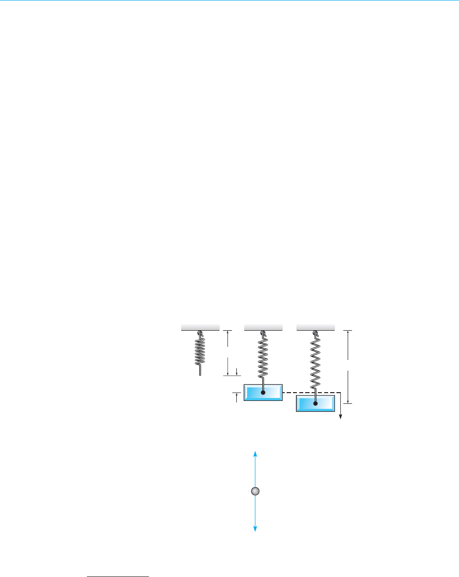
August 7, 2012 21:04 c03 Sheet number 57 Page number 193 cyan black
3.7 Mechanical and Electrical Vibrations 193
how to solve the initial value problem (1), it is only necessary to make appropriate
interpretations of the constants a, b, and c, and of the functions y and g, to obtain
solutions of different physical problems.
We will study the motion of a mass on a spring in detail because understanding the
behavior of this simple system is the first step in the investigation of more complex
vibrating systems. Further, the principles involved are common to many problems.
Consider a mass m hanging at rest on the end of a vertical spring of original length
l, as shown in Figure 3.7.1. The mass causes an elongation L of the spring in the
downward (positive) direction. In this static situation there are two forces acting at
the point where the mass is attached to the spring; see Figure 3.7.2. The gravitational
force, or weight of the mass, acts downward and has magnitude mg, where g is the
acceleration due to gravity.There is also a force F
s
,due to the spring,that acts upward.
If we assume that the elongation L of the spring is small,the spring force is very nearly
proportional to L; this is known as Hooke’s
8
law. Thus we write F
s
=−kL, where
the constant of proportionality k is called the spring constant, and the minus sign is
due to the fact that the spring force acts in the upward (negative) direction. Since
the mass is in equilibrium, the two forces balance each other, which means that
mg − kL = 0. (2)
For a given weight w = mg, you can measure L and then use Eq. (2) to determine k .
Note that k has the units of force/length.
m
m
u
l + L + u
L
l
FIGURE 3.7.1 A spring–mass system.
F
s
= –kL
w = mg
FIGURE 3.7.2 Force diagram for a spring–mass system.
8
Robert Hooke (1635–1703) was an English scientist with wide-ranging interests. His most important
book, Micrographia, was published in 1665 and described a variety of microscopical observations. Hooke
first published his law of elastic behavior in 1676 as ceiiinosssttuv; in 1678 he gave the interpretation ut
tensio sic vis, which means, roughly, “as the force so is the displacement.”

August 7, 2012 21:04 c03 Sheet number 58 Page number 194 cyan black
194 Chapter 3. Second Order Linear Equations
In the corresponding dynamic problem, we are interested in studying the motion
of the mass when it is acted on by an external force or is initially displaced. Let
u(t), measured positive downward, denote the displacement of the mass from its
equilibrium position at time t; see Figure 3.7.1. Then u(t) is related to the forces
acting on the mass through Newton’s law of motion
mu
′′
(t) = f (t), (3)
where u
′′
is the acceleration of the mass and f is the net force acting on the mass.
Observe that both u and f are functions of time. In this dynamic problem there are
now four separate forces that must be considered.
1. The weight w = mg of the mass always acts downward.
2. The spring force F
s
is assumed to be proportional to the total elongation L + u of the
spring and always acts to restore the spring to its natural position. If L + u > 0, then
the spring is extended, and the spring force is directed upward. In this case
F
s
=−k(L + u). (4)
On the other hand, if L + u < 0, then the spring is compressed a distance |L + u|, and
the spring force, which is now directed downward, is given by F
s
= k|L + u|. However,
when L + u < 0, it follows that |L + u|=−(L + u),soF
s
is again given by Eq. (4). Thus,
regardless of the position of the mass, the force exerted by the spring is always expressed
by Eq. (4).
3. The damping or resistive force F
d
always acts in the direction opposite to the direction of
motion of the mass. This force may arise from several sources: resistance from the air or
other medium in which the mass moves, internal energy dissipation due to the extension
or compression of the spring, friction between the mass and the guides (if any) that con-
strain its motion to one dimension,ora mechanical device (dashpot) that imparts a resistive
force to the mass. In any case, we assume that the resistive force is proportional to the
speed |du/dt| of the mass; this is usually referred to as viscous damping. If du/dt > 0,
then u is increasing, so the mass is moving downward. Then F
d
is directed upward and is
given by
F
d
(t) =−γu
′
(t), (5)
where γ is a positive constant of proportionality known as the damping constant. On
the other hand, if du/dt < 0, then u is decreasing, the mass is moving upward, and F
d
is
directed downward. In this case, F
d
= γ|u
′
(t)|; since |u
′
(t)|=−u
′
(t), it follows that F
d
(t)
is again given by Eq. (5). Thus, regardless of the direction of motion of the mass, the
damping force is always expressed by Eq. (5).
The damping force may be rather complicated, and the assumption that it is modeled
adequately by Eq. (5) may be open to question. Some dashpots do behave as Eq. (5)
states, and if the other sources of dissipation are small, it may be possible to neglect
them altogether or to adjust the damping constant γ to approximate them. An important
benefit of the assumption (5) is that it leads to a linear (rather than a nonlinear) differential
equation. In turn, this means that a thorough analysis of the system is straightforward, as
we will show in this section and the next.
4. An applied external force F(t) is directed downward or upward as F(t) is positive or
negative. This could be a force due to the motion of the mount to which the spring is
attached, or it could be a force applied directly to the mass. Often the external force
is periodic.

August 7, 2012 21:04 c03 Sheet number 59 Page number 195 cyan black
3.7 Mechanical and Electrical Vibrations 195
Taking account of these forces, we can now rewrite Newton’s law (3) as
mu
′′
(t) = mg + F
s
(t) + F
d
(t) + F(t)
= mg − k[L + u(t)]−γu
′
(t) + F(t). (6)
Since mg − kL = 0 by Eq. (2), it follows that the equation of motion of the mass is
mu
′′
(t) + γu
′
(t) + ku(t) = F(t), (7)
where the constants m, γ, and k are positive. Note that Eq. (7) has the same form as
Eq. (1).
It is important to understand that Eq. (7) is only an approximate equation for the
displacement u(t). In particular, both Eqs. (4) and (5) should be viewed as approx-
imations for the spring force and the damping force, respectively. In our derivation
we have also neglected the mass of the spring in comparison with the mass of the
attached body.
The complete formulation of the vibration problem requires that we specify two
initial conditions,namely, the initial position u
0
and the initial velocity v
0
of the mass:
u(0) = u
0
, u
′
(0) = v
0
. (8)
It follows from Theorem 3.2.1 that these conditions give a mathematical problem
that has a unique solution. This is consistent with our physical intuition that if the
mass is set in motion with a given initial displacement and velocity, then its posi-
tion will be determined uniquely at all future times. The position of the mass is
given (approximately) by the solution of Eq. (7) subject to the prescribed initial
conditions (8).
EXAMPLE
1
A mass weighing 4 lb stretches a spring 2 in. Suppose that the mass is given an additional
6 in displacement in the positive direction and then released. The mass is in a medium that
exerts a viscous resistance of 6 lb when the mass has a velocity of 3 ft/s. Under the assumptions
discussed in this section, formulate the initial value problem that governs the motion of the
mass.
The required initial value problem consists of the differential equation (7) and initial condi-
tions (8), so our task is to determine the various constants that appear in these equations. The
first step is to choose the units of measurement. Based on the statement of the problem, it is
natural to use the English rather than the metric system of units. The only time unit mentioned
is the second, so we will measure t in seconds. On the other hand, both the foot and the inch
appear in the statement as units of length. It is immaterial which one we use, but having made
a choice, we must be consistent. To be definite, let us measure the displacement u in feet.
Since nothing is said in the statement of the problem about an external force, we assume
that F(t) = 0. To determine m, note that
m =
w
g
=
4 lb
32 ft/s
2
=
1
8
lb·s
2
ft
.
The damping coefficient γ is determined from the statement that γu
′
is equal to 6 lb when u
′
is 3 ft/s. Therefore,
γ =
6 lb
3 ft/s
= 2
lb·s
ft
.

August 7, 2012 21:04 c03 Sheet number 60 Page number 196 cyan black
196 Chapter 3. Second Order Linear Equations
The spring constant k is found from the statement that the mass stretches the spring by 2 in,
or 1/6 ft. Thus
k =
4 lb
1/6 ft
= 24
lb
ft
.
Consequently, Eq. (7) becomes
1
8
u
′′
+ 2u
′
+ 24u = 0,
or
u
′′
+ 16u
′
+ 192u = 0. (9)
The initial conditions are
u(0) =
1
2
, u
′
(0) = 0. (10)
The second initial condition is implied by the word “released” in the statement of the problem,
which we interpret to mean that the mass is set in motion with no initial velocity.
Undamped Free Vibrations. If there is no external force, then F(t) = 0 in Eq. (7). Let
us also suppose that there is no damping, so that γ = 0; this is an idealized config-
uration of the system, seldom (if ever) completely attainable in practice. However,
if the actual damping is very small, then the assumption of no damping may yield
satisfactory results over short to moderate time intervals. In this case the equation
of motion (7) reduces to
mu
′′
+ ku = 0. (11)
The characteristic equation for Eq. (11) is
mr
2
+ k = 0
and its roots are r =±i
!
k/m. Thus the general solution of Eq. (11) is
u = A cosω
0
t + B sin ω
0
t, (12)
where
ω
2
0
= k/m. (13)
The arbitrary constants A and B can be determined if initial conditions of the form
(8) are given.
In discussing the solution of Eq. (11), it is convenient to rewrite Eq. (12) in the
form
u = R cos(ω
0
t − δ), (14)
or
u = R cosδ cos ω
0
t + R sin δ sin ω
0
t. (15)
By comparing Eq. (15) with Eq. (12), we find that A, B, R, and δ are related by the
equations
A = R cosδ, B = R sin δ. (16)
Thus
R =
!
A
2
+ B
2
, tan δ = B/A. (17)
In calculating δ, we must take care to choose the correct quadrant; this can be done
by checking the signs of cos δ and sin δ in Eqs. (16).

August 7, 2012 21:04 c03 Sheet number 61 Page number 197 cyan black
3.7 Mechanical and Electrical Vibrations 197
The graphof Eq. (14),or the equivalent Eq.(12),fora typicalset of initialconditions
is shown in Figure 3.7.3.Thegraph isa displacedcosine wavethat describesa periodic,
or simple harmonic, motion of the mass. The period of the motion is
T =
2π
ω
0
= 2π
)
m
k
*
1/2
. (18)
The circular frequency ω
0
=
!
k/m, measured in radians per unit time, is called the
natural frequency of the vibration. The maximum displacement R of the mass from
equilibrium is the amplitude of the motion. The dimensionless parameter δ is called
the phase,or phase angle,and measures the displacement of the wave from its normal
position corresponding to δ = 0.
R
u
–R
δ
R cos
δ
+ 2
π
δ
+
π
δ
0
t
ω
FIGURE 3.7.3 Simple harmonic motion; u = R cos(ω
0
t − δ).
Note that the motion described by Eq. (14) has a constant amplitude that does not
diminish with time. This reflects the fact that, in the absence of damping, there is no
way for the system to dissipate the energy imparted to it by the initial displacement
and velocity. Further, for a given mass m and spring constant k, the system always
vibrates at the same frequency ω
0
, regardless of the initial conditions. However, the
initial conditions do help to determine the amplitude of the motion. Finally, observe
from Eq. (18) that T increases as m increases, so larger masses vibrate more slowly.
On the other hand, T decreases as k increases, which means that stiffer springs cause
the system to vibrate more rapidly.
EXAMPLE
2
Suppose that a mass weighing 10 lb stretches a spring 2 in. If the mass is displaced an additional
2 in and is then set in motion with an initial upward velocity of 1 ft/s, determine the position
of the mass at any later time. Also determine the period, amplitude, and phase of the motion.
The spring constant is k = 10 lb/2in= 60 lb/ft, and the mass is m = w/g = 10/32 lb·s
2
/ft.
Hence the equation of motion reduces to
u
′′
+ 192u = 0, (19)
and the general solution is
u = A cos(8
√
3t) + B sin(8
√
3t).
The solution satisfying the initial conditions u(0) = 1/6 ft and u
′
(0) =−1 ft/s is
u =
1
6
cos(8
√
3t) −
1
8
√
3
sin(8
√
3t). (20)

August 7, 2012 21:04 c03 Sheet number 62 Page number 198 cyan black
198 Chapter 3. Second Order Linear Equations
The natural frequency is ω
0
=
√
192
∼
=
13.856 rad/s, so the period is T = 2π/ω
0
∼
=
0.45345 s.
The amplitude R and phase δ are found from Eqs. (17). We have
R
2
=
1
36
+
1
192
=
19
576
,soR
∼
=
0.18162 ft.
The second of Eqs. (17) yields tan δ =−
√
3/4. There are two solutions of this equation, one in
the second quadrant and one in the fourth. In the present problem, cos δ>0 and sin δ<0, so
δ is in the fourth quadrant. In fact,
δ =−arctan(
√
3/4)
∼
=
−0.40864 rad.
The graph of the solution (20) is shown in Figure 3.7.4.
0.2
– 0.2
1.5
T = 0.453
~
u = 0.182 cos(8√3 t + 0.409)
R = 0.182
~
u
t
FIGURE 3.7.4 An undamped free vibration: u
′′
+ 192u = 0, u(0) = 1/6, u
′
(0) =−1.
Damped Free Vibrations. If we include the effect of damping, the differential equation
governing the motion of the mass is
mu
′′
+ γu
′
+ ku = 0. (21)
We are especially interested in examining the effect of variations in the damping
coefficient γ for given values of the mass m and spring constant k. The corresponding
characteristic equation is
mr
2
+ γr + k = 0,
and its roots are
r
1
, r
2
=
−γ ±
!
γ
2
− 4km
2m
=
γ
2m
#
−1 ±
+
1 −
4km
γ
2
$
. (22)
Depending on the sign of γ
2
− 4km, the solution u has one of the following forms:
γ
2
− 4km > 0, u = Ae
r
1
t
+ Be
r
2
t
; (23)
γ
2
− 4km = 0, u = (A + Bt)e
−γt/2m
; (24)
γ
2
− 4km < 0, u = e
−γt/2m
(A cos µt + B sin µt), µ =
(4km − γ
2
)
1/2
2m
> 0. (25)
Since m, γ, and k are positive, γ
2
− 4km is always less than γ
2
. Hence,
if γ
2
− 4km ≥ 0, then the values of r
1
and r
2
given by Eq. (22) are negative.If
γ
2
− 4km < 0, then the values of r
1
and r
2
are complex, but with negative real part.
Thus, in all cases, the solution u tends to zero as t →∞; this occurs regardless of the

August 7, 2012 21:04 c03 Sheet number 63 Page number 199 cyan black
3.7 Mechanical and Electrical Vibrations 199
values of the arbitrary constants A and B—that is, regardless of the initial conditions.
This confirms our intuitive expectation, namely, that damping gradually dissipates
the energy initially imparted to the system, and consequently the motion dies out
with increasing time.
The most important case is the third one, which occurs when the damping is small.
If we let A = R cosδ and B = R sin δ in Eq. (25), then we obtain
u = Re
−γt/2m
cos(µt − δ). (26)
The displacement u lies between the curves u =±Re
−γt/2m
; hence it resembles a
cosine wave whose amplitude decreases as t increases. A typical example is sketched
in Figure 3.7.5. The motion is called a damped oscillation or a damped vibration. The
amplitude factor R depends on m, γ, k, and the initial conditions.
u
δ
+ 3
δ
R cos
Re
– t/2m
γ
−Re
– t/2m
t
µ
δ π
+ 2
δ π
δ π
+
FIGURE 3.7.5 Damped vibration; u = Re
−γt/2m
cos(µt − δ).
Although the motion is not periodic, the parameter µ determines the frequency
with which the mass oscillates back and forth; consequently, µ is called the quasi
frequency. By comparing µ with the frequency ω
0
of undamped motion, we find that
µ
ω
0
=
(4km − γ
2
)
1/2
/2m
!
k/m
=
'
1 −
γ
2
4km
(
1/2
∼
=
1 −
γ
2
8km
. (27)
The last approximation is valid when γ
2
/4km is small; we refer to this situation as
“small damping.”Thus the effect of small damping is to reduce slightly the frequency
of the oscillation. By analogy with Eq. (18), the quantity T
d
= 2π/µ is called the
quasi period. It is the time between successive maxima or successive minima of
the position of the mass, or between successive passages of the mass through its
equilibrium position while going in the same direction. The relation between T
d
and
T is given by
T
d
T
=
ω
0
µ
=
'
1 −
γ
2
4km
(
−1/2
∼
=
'
1 +
γ
2
8km
(
, (28)
where again the lastapproximation is valid whenγ
2
/4km is small.Thussmall damping
increases the quasi period.
Equations (27) and (28) reinforce the significance of the dimensionless ratio
γ
2
/4km. It is not the magnitude of γ alone that determines whether damping is large
or small, but the magnitude of γ
2
compared to 4km. When γ
2
/4km is small, then
damping has a small effect on the quasi frequency and quasi period of the motion.

August 7, 2012 21:04 c03 Sheet number 64 Page number 200 cyan black
200 Chapter 3. Second Order Linear Equations
On the other hand, if we want to study the detailed motion of the mass for all time,
then we can never neglect the damping force, no matter how small.
As γ
2
/4km increases, the quasi frequency µ decreases and the quasi period T
d
increases. In fact, µ → 0 and T
d
→∞as γ → 2
√
km. As indicated by Eqs. (23), (24),
and (25), the nature of the solution changes as γ passes through the value 2
√
km.
The motion with γ = 2
√
km is said to be critically damped. For larger values of γ
the motion is said to be overdamped. In these cases, given by Eqs. (24) and (23),
respectively, the mass may pass through its equilibrium position at most once (see
Figure3.7.6) andthen creeps back toit.The massdoes notoscillate about equilibrium,
as it does for small γ. Two typical examples of critically damped motion are shown
in Figure 3.7.6, and the situation is discussed further in Problems 21 and 22.
2
1
–1
2 4 6 10
8
u
t
u(0) = , u'(0) =
1
2
7
4
u = + 2t e
–t/2
1
2
(
)
u(0) = , u'
1
2
7
4
u = – t e
–t/2
1
2
3
2
(
)
FIGURE 3.7.6 Critically damped motions: u
′′
+ u
′
+ 0.25u = 0; u = (A + Bt)e
−t/2
.
EXAMPLE
3
The motion of a certain spring–mass system is governed by the differential equation
u
′′
+ 0.125u
′
+ u = 0, (29)
where u is measured in feet and t in seconds. If u(0) = 2 and u
′
(0) = 0, determine the position
of the mass at any time. Find the quasi frequency and the quasi period, as well as the time
at which the mass first passes through its equilibrium position. Also find the time τ such that
|u(t)| < 0 .1 for all t >τ.
The solution of Eq. (29) is
u = e
−t/16
,
A cos
√
255
16
t + B sin
√
255
16
t
-
.
To satisfy the initial conditions, we must choose A = 2 and B = 2/
√
255; hence the solution of
the initial value problem is
u = e
−t/16
#
2 cos
√
255
16
t +
2
√
255
sin
√
255
16
t
$
=
32
√
255
e
−t/16
cos
#
√
255
16
t − δ
$
, (30)

August 7, 2012 21:04 c03 Sheet number 65 Page number 201 cyan black
3.7 Mechanical and Electrical Vibrations 201
2
1
–1
–2
u
t
u" + u
u" + 0.125 u' + u = 0
u(0) = 2, u' (0) = 0
10 20 30 40 50
FIGURE 3.7.7 Vibration with small damping (solid curve)
and with no damping (dashed curve).
where tan δ = 1/
√
255, so δ
∼
=
0.06254. The displacement of the mass as a function of time is
shown in Figure 3.7.7. For purposes of comparison, we also show the motion if the damping
term is neglected.
The quasi frequency is µ =
√
255/16
∼
=
0.998, and the quasi period is T
d
= 2π/µ
∼
=
6.295 s.
These values differ only slightly from the corresponding values (1 and 2π, respectively) for
the undamped oscillation. This is evident also from the graphs in Figure 3.7.7, which rise
and fall almost together. The damping coefficient is small in this example: only one-sixteenth
of the critical value, in fact. Nevertheless, the amplitude of the oscillation is reduced rather
rapidly. Figure 3.7.8 shows the graph of the solution for 40 ≤ t ≤ 60, together with the graphs
of u =±0.1. From the graph it appears that τ is about 47.5, and by a more precise calculation
we find that τ
∼
=
47.5149 s.
0.1
0.05
–0.05
–0.1
–0.15
40 45 50 55 60
τ
u = –0.1
u = 0.1
u = e
–t/16
cos t – 0.06254
32
√255
16
√255
()
u
t
FIGURE 3.7.8 Solution of Example 3; determination of the time τ after which |u(t)| < 0.1.

August 7, 2012 21:04 c03 Sheet number 66 Page number 202 cyan black
202 Chapter 3. Second Order Linear Equations
To find the time at which the mass first passes through its equilibrium position, we refer to
Eq. (30) and set
√
255t/16 − δ equal to π/2, the smallest positive zero of the cosine function.
Then, by solving for t, we obtain
t =
16
√
255
)
π
2
+ δ
*
∼
=
1.637 s.
Electric Circuits. A second example of the occurrence of second order linear differen-
tial equations with constant coefficients is their use as a model of the flow of electric
current in the simple series circuit shown in Figure 3.7.9. The current I, measured
in amperes (A), is a function of time t. The resistance R in ohms (4), the capaci-
tance C in farads (F), and the inductance L in henrys (H) are all positive and are
assumed to be known constants. The impressed voltage E in volts (V) is a given func-
tion of time. Another physical quantity that enters the discussion is the total charge
Q in coulombs (C) on the capacitor at time t. The relation between charge Q and
current I is
I = dQ/dt. (31)
Resistance R Capacitance C
Inductance L
Impressed voltage E(t)
I
FIGURE 3.7.9 A simple electric circuit.
The flow of current in the circuit is governed by Kirchhoff’s
9
second law:In a closed
circuit the impressed voltage is equal to the sum of the voltage drops in the rest of the
circuit.
According to the elementary laws of electricity, we know that
The voltage drop across the resistor is IR.
The voltage drop across the capacitor is Q/C.
The voltage drop across the inductor is LdI/dt.
Hence, by Kirchhoff’s law,
L
dI
dt
+ RI +
1
C
Q = E(t). (32)
9
Gustav Kirchhoff (1824–1887) was a German physicist and professor at Breslau, Heidelberg, and Berlin.
He formulated the basic laws of electric circuits about 1845 while still a student at Albertus University in
his native Königsberg. In 1857 he discovered that an electric current in a resistanceless wire travels at the
speed of light. He is also famous for fundamental work in electromagnetic absorption and emission and
was one of the founders of spectroscopy.

August 7, 2012 21:04 c03 Sheet number 67 Page number 203 cyan black
3.7 Mechanical and Electrical Vibrations 203
The units for voltage, resistance, current, charge, capacitance, inductance, and time
are all related:
1 volt = 1 ohm · 1 ampere = 1 coulomb/1 farad = 1 henry · 1 ampere/1 second.
Substituting for I from Eq. (31), we obtain the differential equation
LQ
′′
+ RQ
′
+
1
C
Q = E(t) (33)
for the charge Q. The initial conditions are
Q(t
0
) = Q
0
, Q
′
(t
0
) = I(t
0
) = I
0
. (34)
Thus we must know the charge on the capacitor and the current in the circuit at some
initial time t
0
.
Alternatively, we can obtain a differential equation for the current I by differen-
tiating Eq. (33) with respect to t, and then substituting for dQ/dt from Eq. (31). The
result is
LI
′′
+ RI
′
+
1
C
I = E
′
(t), (35)
with the initial conditions
I(t
0
) = I
0
, I
′
(t
0
) = I
′
0
. (36)
From Eq. (32) it follows that
I
′
0
=
E(t
0
) − RI
0
− (1/C)Q
0
L
. (37)
Hence I
′
0
is also determined by the initial charge and current, which are physically
measurable quantities.
The most important conclusion from this discussion is that the flow of current in the
circuit is described by an initial value problem of precisely the same form as the one
that describes the motion of a spring–mass system. This is a good example of the uni-
fying role of mathematics:once you know how to solve second order linear equations
with constant coefficients, you can interpret the results in terms of mechanical vibra-
tions, electric circuits, or any other physical situation that leads to the same problem.
PROBLEMS In each of Problems 1 through 4, determine ω
0
, R, and δ so as to write the given expression in
the form u = R cos(ω
0
t − δ).
1. u = 3 cos 2t + 4 sin 2t 2. u =−cos t +
√
3 sin t
3. u = 4 cos 3t − 2 sin 3t 4. u =−2 cos πt − 3 sin πt
5.
A mass weighing 2 lb stretches a spring 6 in. If the mass is pulled down an additional 3 in
and then released, and if there is no damping, determine the position u of the mass at any
time t. Plot u versus t. Find the frequency, period, and amplitude of the motion.
6. A mass of 100 g stretches a spring 5 cm. If the mass is set in motion from its equilibrium posi-
tion with a downwardvelocity of 10cm/s,andif there isno damping,determine theposition
u of the mass at any time t. When does the mass first return to its equilibrium position?
7. A mass weighing 3 lb stretches a spring 3 in. If the mass is pushed upward, contracting
the spring a distance of 1 in, and then set in motion with a downward velocity of 2 ft/s,
and if there is no damping, find the position u of the mass at any time t. Determine the
frequency, period, amplitude, and phase of the motion.

August 7, 2012 21:04 c03 Sheet number 68 Page number 204 cyan black
204 Chapter 3. Second Order Linear Equations
8. A series circuit has a capacitor of 0.25 × 10
−6
F and an inductor of 1 H. If the initial charge
on the capacitor is 10
−6
C and there is no initial current, find the charge Q on the capacitor
at any time t.
9.
A mass of 20 g stretches a spring 5 cm. Suppose that the mass is also attached to a viscous
damper with a damping constant of 400 dyn·s/cm. If the mass is pulled down an additional
2 cm and then released,find its position u at any time t. Plot u versus t. Determine the quasi
frequency and the quasi period. Determine the ratio of the quasi period to the period of
the corresponding undamped motion. Also find the time τ such that |u(t)| < 0.05 cm for
all t >τ.
10.
A mass weighing 16 lb stretches a spring 3 in. The mass is attached to a viscous damper
with a damping constant of 2 lb·s/ft. If the mass is set in motion from its equilibrium posi-
tion with a downward velocity of 3 in/s, find its position u at any time t. Plot u versus t.
Determine when the mass first returns to its equilibrium position. Also find the time τ
such that |u(t)| < 0.01 in for all t >τ.
11. A spring is stretched 10 cm by a force of 3 N. A mass of 2 kg is hung from the spring and
is also attached to a viscous damper that exerts a force of 3 N when the velocity of the
mass is 5 m/s. If the mass is pulled down 5 cm below its equilibrium position and given an
initial downward velocity of 10 cm/s, determine its position u at any time t. Find the quasi
frequency µ and the ratio of µ to the natural frequency of the corresponding undamped
motion.
12. A series circuit has a capacitor of 10
−5
F, a resistor of 3 × 10
2
4, and an inductor of 0.2 H.
The initial charge on the capacitor is 10
−6
C and there is no initial current. Find the charge
Q on the capacitor at any time t.
13. A certain vibrating system satisfies the equation u
′′
+ γu
′
+ u = 0. Find the value of the
damping coefficient γ for which the quasi period of the damped motion is 50% greater
than the period of the corresponding undamped motion.
14. Show that the period of motion of an undamped vibration of a mass hanging from a ver-
tical spring is 2π
!
L/g, where L is the elongation of the spring due to the mass, and g is
the acceleration due to gravity.
15. Show that the solution of the initial value problem
mu
′′
+ γu
′
+ ku = 0, u(t
0
) = u
0
, u
′
(t
0
) = u
′
0
can be expressed as the sum u = v + w, where v satisfies the initial conditions
v(t
0
) = u
0
, v
′
(t
0
) = 0, w satisfies the initial conditions w(t
0
) = 0, w
′
(t
0
) = u
′
0
, and both v
and w satisfy the same differential equation as u. This is another instance of superposing
solutions of simpler problems to obtain the solution of a more general problem.
16. Show that A cos ω
0
t + B sin ω
0
t can be written in the form r sin(ω
0
t − θ). Determine r and
θ in terms of A and B.IfR cos(ω
0
t − δ) = r sin(ω
0
t − θ), determine the relationship among
R, r, δ, and θ.
17. A mass weighing 8 lb stretches a spring 1.5 in. The mass is also attached to a damper with
coefficient γ. Determine the value of γ for which the system is critically damped; be sure
to give the units for γ.
18. If a series circuit has a capacitor of C = 0.8 × 10
−6
F and an inductor of L = 0.2 H, find
the resistance R so that the circuit is critically damped.
19. Assume that the system described by the equation mu
′′
+ γu
′
+ ku = 0 is either critically
damped or overdamped. Show that the mass can pass through the equilibrium position at
most once, regardless of the initial conditions.
Hint: Determine all possible values of t for which u = 0.

August 7, 2012 21:04 c03 Sheet number 69 Page number 205 cyan black
3.7 Mechanical and Electrical Vibrations 205
20. Assume thatthe system describedby the equationmu
′′
+ γu
′
+ ku = 0 iscritically damped
and that the initial conditionsare u(0) = u
0
, u
′
(0) = v
0
.Ifv
0
= 0,show that u → 0ast →∞
but that u is never zero. If u
0
is positive, determine a condition on v
0
that will ensure that
the mass passes through its equilibrium position after it is released.
21. Logarithmic Decrement. (a) For the damped oscillation described by Eq. (26), show
that the time between successive maxima is T
d
= 2π/µ.
(b) Show that the ratio of the displacements at two successive maxima is given by
exp(γT
d
/2m). Observe that this ratio does not depend on which pair of maxima
is chosen. The natural logarithm of this ratio is called the logarithmic decrement and is
denoted by 5.
(c) Show that 5 = πγ/mµ. Since m,µ,and 5 are quantities that can be measured easily for
a mechanical system, this result provides a convenient and practical method for determin-
ing the damping constant of the system, which is more difficult to measure directly. In par-
ticular,for the motion of a vibrating mass in a viscous fluid,the damping constant depends
on the viscosity of the fluid; for simple geometric shapes the form of this dependence is
known, and the preceding relation allows the experimental determination of the viscosity.
This is one of the most accurate ways of determining the viscosity of a gas at high pressure.
22. Referring to Problem 21, find the logarithmic decrement of the system in Problem 10.
23. For the system in Problem 17, suppose that 5 = 3 and T
d
= 0.3 s. Referring to Problem
21, determine the value of the damping coefficient γ.
24. The position of a certain spring–mass system satisfies the initial value problem
3
2
u
′′
+ ku = 0, u(0) = 2, u
′
(0) = v.
If the period andamplitude of theresulting motionare observed tobe π and 3,respectively,
determine the values of k and v.
25.
Consider the initial value problem
u
′′
+ γu
′
+ u = 0, u(0) = 2, u
′
(0) = 0.
We wish to explore how long a time interval is required for the solution to become “neg-
ligible” and how this interval depends on the damping coefficient γ. To be more precise,
let us seek the time τ such that |u(t)| < 0.01 for all t >τ. Note that critical damping for
this problem occurs for γ = 2.
(a) Let γ = 0.25 and determine τ, or at least estimate it fairly accurately from a plot of
the solution.
(b) Repeat part (a) for several other values of γ in the interval 0 <γ<1.5. Note that τ
steadily decreases as γ increases for γ in this range.
(c) Create a graph of τ versus γ by plotting the pairs of values found in parts (a) and (b).
Is the graph a smooth curve?
(d) Repeat part (b) for values of γ between 1.5 and 2. Show that τ continues to decrease
until γ reaches a certain critical value γ
0
, after which τ increases. Find γ
0
and the
corresponding minimum value of τ to two decimal places.
(e) Another way to proceed is to write the solution of the initial value problem in
the form (26). Neglect the cosine factor and consider only the exponential factor and the
amplitude R. Then find an expression for τ as a function of γ. Compare the approximate
results obtained in this way with the values determined in parts (a), (b), and (d).
26. Consider the initial value problem
mu
′′
+ γu
′
+ ku = 0, u(0) = u
0
, u
′
(0) = v
0
.
Assume that γ
2
< 4km.

August 7, 2012 21:04 c03 Sheet number 70 Page number 206 cyan black
206 Chapter 3. Second Order Linear Equations
(a) Solve the initial value problem.
(b) Write the solution in the form u(t) = R exp(−γt/2m) cos(µt − δ). Determine R in
terms of m, γ, k, u
0
, and v
0
.
(c) Investigate the dependence of R on the damping coefficient γ for fixed values of the
other parameters.
27. A cubic block of side l and mass density ρ per unit volume is floating in a fluid of mass den-
sity ρ
0
per unit volume, where ρ
0
>ρ. If the block is slightly depressed and then released,
it oscillates in the vertical direction. Assuming that the viscous damping of the fluid and
air can be neglected, derive the differential equation of motion and determine the period
of the motion.
Hint: Use Archimedes’
10
principle: an object that is completely or partially submerged
in a fluid is acted on by an upward (buoyant) force equal to the weight of the displaced
fluid.
28.
The position of a certain undamped spring–mass system satisfies the initial value problem
u
′′
+ 2u = 0, u(0) = 0, u
′
(0) = 2.
(a) Find the solution of this initial value problem.
(b) Plot u versus t and u
′
versus t on the same axes.
(c) Plot u
′
versus u; that is, plot u(t) and u
′
(t) parametrically with t as the parameter.
This plot is known as a phase plot, and the uu
′
-plane is called the phase plane. Observe
that a closed curve in the phase plane corresponds to a periodic solution u(t). What is the
direction of motion on the phase plot as t increases?
29.
The position of a certain spring–mass system satisfies the initial value problem
u
′′
+
1
4
u
′
+ 2u = 0, u(0) = 0, u
′
(0) = 2.
(a) Find the solution of this initial value problem.
(b) Plot u versus t and u
′
versus t on the same axes.
(c) Plot u
′
versus u in the phase plane (see Problem 28). Identify several corresponding
points on the curves in parts (b) and (c). What is the direction of motion on the phase plot
as t increases?
30. In the absence of damping, the motion of a spring–mass system satisfies the initial value
problem
mu
′′
+ ku = 0, u(0) = a, u
′
(0) = b.
(a) Show that the kinetic energy initially imparted to the mass is mb
2
/2 and that the
potential energy initially stored in the spring is ka
2
/2, so that initially the total energy in
the system is (ka
2
+ mb
2
)/2.
(b) Solve the given initial value problem.
(c) Using the solution in part (b), determine the total energy in the system at any time t.
Your result should confirm the principle of conservation of energy for this system.
10
Archimedes (287–212 BC) was the foremost of the ancient Greek mathematicians. He lived in Syracuse
on the island of Sicily. His most notable discoveries were in geometry, but he also made important contri-
butions to hydrostatics and other branches of mechanics. His method of exhaustion is a precursor of the
integral calculus developed by Newton and Leibniz almost two millennia later. He died at the hands of a
Roman soldier during the Second Punic War.

August 7, 2012 21:04 c03 Sheet number 71 Page number 207 cyan black
3.8 Forced Vibrations 207
31. Suppose that a mass m slides without friction on a horizontal surface.The mass is attached
to a spring with spring constant k , as shown in Figure 3.7.10, and is also subject to viscous
air resistance with coefficient γ. Show that the displacement u(t) of the mass from its
equilibrium position satisfies Eq. (21). How does the derivation of the equation of motion
in this case differ from the derivation given in the text?
k
m
u(t)
FIGURE 3.7.10 A spring–mass system.
32.
In the spring–mass system of Problem 31, suppose that the spring force is not given by
Hooke’s law but instead satisfies the relation
F
s
=−(ku + ϵu
3
),
where k > 0 and ϵ is small but may be of either sign.The spring is called a hardening spring
if ϵ>0 and a softening spring if ϵ<0. Why are these terms appropriate?
(a) Show that the displacement u(t) of the mass from its equilibrium position satisfies the
differential equation
mu
′′
+ γu
′
+ ku + ϵu
3
= 0.
Suppose that the initial conditions are
u(0) = 0, u
′
(0) = 1.
In the remainder of this problem, assume that m = 1, k = 1, and γ = 0.
(b) Find u(t) when ϵ = 0 and also determine the amplitude and period of the motion.
(c) Let ϵ = 0.1. Plot a numerical approximation to the solution. Does the motion appear
to be periodic? Estimate the amplitude and period.
(d) Repeat part (c) for ϵ = 0.2 and ϵ = 0.3.
(e) Plot your estimated values of the amplitude A and the period T versus ϵ. Describe
the way in which A and T, respectively, depend on ϵ.
(f) Repeat parts (c), (d), and (e) for negative values of ϵ.
3.8 Forced Vibrations
We will now investigate the situation in which a periodic external force is applied
to a spring–mass system. The behavior of this simple system models that of many
oscillatory systems with an external force due, for example, to a motor attached to
the system. We will first consider the case in which damping is present and will look
later at the idealized special case in which there is assumed to be no damping.
Forced Vibrations with Damping. The algebraic calculations can be fairly complicated in
this kind of problem, so we will begin with a relatively simple example.

August 7, 2012 21:04 c03 Sheet number 72 Page number 208 cyan black
208 Chapter 3. Second Order Linear Equations
EXAMPLE
1
Suppose that the motion of a certain spring–mass system satisfies the differential equation
u
′′
+ u
′
+ 1.25u = 3 cos t (1)
and the initial conditions
u(0) = 2, u
′
(0) = 3. (2)
Find the solution of this initial value problem and describe the behavior of the solution for
large t.
The homogeneous equation corresponding to Eq. (1) has the characteristic equation
r
2
+ r + 1.25 = 0 with roots r =−0.5 ± i. Thus the general solution u
c
(t) of this homogeneous
equation is
u
c
(t) = c
1
e
−t/2
cos t + c
2
e
−t/2
sin t. (3)
A particular solution of Eq. (1) has the form U(t) = A cos t + B sin t, where A and B
are found by substituting U(t) for u in Eq. (1). We have U
′
(t) =−A sin t + B cos t and
U
′′
(t) =−A cos t − B sin t. Thus, from Eq. (1) we obtain
(0.25A + B) cos t + (−A + 0.25B) sin t = 3 cos t.
Consequently, A and B must satisfy the equations
0.25A + B = 3, −A + 0.25B = 0,
with the result that A = 12/17 and B = 48/17. Therefore, the particular solution is
U(t) =
12
17
cos t +
48
17
sin t, (4)
and the general solution of Eq. (1) is
u = u
c
(t) + U(t) = c
1
e
−t/2
cos t + c
2
e
−t/2
sin t +
12
17
cos t +
48
17
sin t. (5)
The remaining constants c
1
and c
2
are determined by the initial conditions (2). From Eq. (5)
we have
u(0) = c
1
+
12
17
= 2, u
′
(0) =−
1
2
c
1
+ c
2
+
48
17
= 3,
so c
1
= 22/17 and c
2
= 14/17. Thus we finally obtain the solution of the given initial value
problem, namely,
u =
22
17
e
−t/2
cos t +
14
17
e
−t/2
sin t +
12
17
cos t +
48
17
sin t. (6)
The graph of the solution (6) is shown by the black curve in Figure 3.8.1.
It is important to note that the solution consists of two distinct parts. The first two terms on
the right side of Eq. (6) contain the exponential factor e
−t/2
; as a result they rapidly approach
zero. It is customary to call these terms transient. The remaining terms in Eq. (6) involve only
sines and cosines, so they represent an oscillation that continues indefinitely. We refer to them
as a steady state. The solid and dashed blue curves in Figure 3.8.1 show the transient and the
steady state parts of the solution, respectively. The transient part comes from the solution
of the homogeneous equation corresponding to Eq. (1) and is needed to satisfy the initial
conditions. The steady state is the particular solution of the full nonhomogeneous equation.
After a fairly short time, the transient is vanishingly small and the full solution is essentially
indistinguishable from the steady state.

August 7, 2012 21:04 c03 Sheet number 73 Page number 209 cyan black
3.8 Forced Vibrations 209
u
t
2
1
–1
–2
–3
3
128614
Full solution
Steady state
Transient
FIGURE 3.8.1 Solution of the initial value problem (1), (2):
u
′′
+ u
′
+ 1.25u = 3 cos t, u(0) = 2, u
′
(0) = 3.
The equation of motion of a general spring–mass system subject to an external
force F(t) is [Eq. (7) in Section 3.7]
mu
′′
(t) + γu
′
(t) + ku(t) = F(t), (7)
where m,γ,and k are the mass,damping coefficient,and springconstant of the spring–
mass system. Suppose now that the external force is given by F
0
cos ωt, where F
0
and
ω are positive constants representing the amplitude and frequency, respectively, of
the force. Then Eq. (7) becomes
mu
′′
+ γu
′
+ ku = F
0
cos ωt. (8)
Solutions of Eq. (8) behave very much like the solution in the preceding example.
The general solution of Eq. (8) must have the form
u = c
1
u
1
(t) + c
2
u
2
(t) + A cos ω t + B sin ωt = u
c
(t) + U(t). (9)
The first two terms on the right side of Eq. (9) are the general solution u
c
(t) of
the homogeneous equation corresponding to Eq. (8), and the latter two terms are
a particular solution U(t) of the full nonhomogeneous equation. The coefficients
A and B can be found, as usual, by substituting these terms into the differen-
tial equation (8), while the arbitrary constants c
1
and c
2
are available to satisfy
initial conditions, if any are prescribed. The solutions u
1
(t) and u
2
(t) of the homo-
geneous equation depend on the roots r
1
and r
2
of the characteristic equation
mr
2
+ γr + k = 0. Since m, γ, and k are all positive, it follows that r
1
and r
2
either
are real and negative or are complex conjugates with negative real part. In either
case, both u
1
(t) and u
2
(t) approach zero as t →∞. Since u
c
(t) dies out as t increases,
it is called the transient solution. In many applications, it is of little importance and
(depending on the value of γ) may well be undetectable after only a few seconds.
The remaining terms in Eq. (9)—namely, U(t) = A cos ωt + B sin ωt—do not die
out as t increases but persist indefinitely, or as long as the external force is applied.

August 7, 2012 21:04 c03 Sheet number 74 Page number 210 cyan black
210 Chapter 3. Second Order Linear Equations
They represent a steady oscillation with the same frequency as the external force
and are called the steady state solution or the forced response.The transient solution
enables us to satisfy whatever initial conditions may be imposed. With increasing
time, the energy put into the system by the initial displacement and velocity is dis-
sipated through the damping force, and the motion then becomes the response of
the system to the external force. Without damping,the effect of the initial conditions
would persist for all time.
It is convenient to express U(t) as a single trigonometric term rather than as a sum
of two terms. Recall that we did this for other similar expressions in Section 3.7. Thus
we write
U(t) = R cos(ωt − δ). (10)
The amplitude R and phase δ depend directly on A and B and indirectly on the
parameters in the differential equation (8). It is possible to show, by straightforward
but somewhat lengthy algebraic computations, that
R =
F
0
5
, cos δ =
m(ω
2
0
− ω
2
)
5
, sin δ =
γω
5
, (11)
where
5 =
?
m
2
(ω
2
0
− ω
2
)
2
+ γ
2
ω
2
and ω
2
0
= k/m. (12)
Recall that ω
0
is the natural frequency of the unforced system in the absence of
damping.
We now investigate how the amplitude R of the steady state oscillation depends on
the frequency ω of the external force. Substituting from Eq. (12) into the expression
for R in Eq. (11) and executing some algebraic manipulations, we find that
Rk
F
0
= 1
@,
'
1 −
ω
2
ω
2
0
(
2
+ 2
ω
2
ω
2
0
-
1/2
, (13)
where 2 = γ
2
/mk. Observe that the quantity Rk/F
0
is the ratio of the amplitude R
of the forced response to F
0
/k, the static displacement of the spring produced by a
force F
0
.
For low frequency excitation—that is, as ω → 0—it follows from Eq. (13) that
Rk/F
0
→ 1orR → F
0
/k. At the other extreme, for very high frequency excitation,
Eq. (13) implies that R → 0asω →∞. At an intermediate value of ω the amplitude
may have amaximum.To find this maximumpoint,wecan differentiateR with respect
to ω and set the result equal to zero. In this way we find that the maximum amplitude
occurs when ω = ω
max
, where
ω
2
max
= ω
2
0
−
γ
2
2m
2
= ω
2
0
'
1 −
γ
2
2mk
(
. (14)
Note that ω
max
<ω
0
and that ω
max
is close to ω
0
when γ is small. The maximum
value of R is
R
max
=
F
0
γω
0
!
1 − (γ
2
/4mk)
∼
=
F
0
γω
0
'
1 +
γ
2
8mk
(
, (15)
where the last expression is an approximation for small γ.Ifγ
2
/mk > 2, then ω
max
as
given by Eq. (14) is imaginary; in this case the maximum value of R occurs for ω = 0,

August 7, 2012 21:04 c03 Sheet number 75 Page number 211 cyan black
3.8 Forced Vibrations 211
and R is a monotone decreasing function of ω. Recall that critical damping occurs
when γ
2
/mk = 4.
For small γ it follows from Eq. (15) that R
max
∼
=
F
0
/γω
0
. Thus, for lightly damped
systems, the amplitude R of the forced response when ω is near ω
0
is quite large
even for relatively small external forces, and the smaller the value of γ, the more
pronounced is this effect. This phenomenon is known as resonance, and it is often
an important design consideration. Resonance can be either good or bad, depending
on the circumstances. It must be taken very seriously in the design of structures,
such as buildings and bridges, where it can produce instabilities that might lead to
the catastrophic failure of the structure. On the other hand, resonance can be put
to good use in the design of instruments, such as seismographs, that are intended to
detect weak periodic incoming signals.
Figure 3.8.2 contains some representative graphs of Rk/F
0
versus ω/ω
0
for several
values of 2 = γ
2
/mk. The graph corresponding to 2 = 0.015625 is included because
this is the value of 2 that occurs in Example 2 below. Note particularly the sharp
peak in the curve corresponding to 2 = 0.015625 near ω/ω
0
= 1. The limiting case
as 2 → 0 is also shown. It follows from Eq. (13), or from Eqs. (11) and (12), that
R → F
0
/m|ω
2
0
− ω
2
| as γ → 0 and hence Rk/F
0
is asymptotic to the vertical line
ω = ω
0
, as shown in the figure. As the damping in the system increases, the peak
response gradually diminishes.
2
4
6
8
10
0.2 0.4 0.6 0.8 1 1.2 1.4 1.6 1.8 2
Γ = 2
Γ = 0.5
Rk/F
0
/
ωω
Γ = 0.1
Γ = 0.015625
Γ
→
0
0
FIGURE 3.8.2 Forced vibration with damping: amplitude of steady
state response versus frequency of driving force; 2 = γ
2
/mk.
Figure3.8.2 also illustrates the usefulnessof dimensionless variables.Youcan easily
verify thateach ofthe quantitiesRk/F
0
,ω/ω
0
,and 2 is dimensionless.The importance
of this observation is that the number of significant parameters in the problem has
been reduced to three rather than the five that appear in Eq. (8). Thus only one
family of curves, of which a few are shown in Figure 3.8.2, is needed to describe the
response-versus-frequency behavior of all systems governed by Eq. (8).
The phase angle δ also depends in aninteresting way on ω.Forω near zero,it follows
from Eqs. (11) and (12) that cos δ
∼
=
1 and sin δ
∼
=
0. Thus δ
∼
=
0, and the response is
nearly in phase with the excitation, meaning that they rise and fall together and,
in particular, assume their respective maxima nearly together and their respective

August 7, 2012 21:04 c03 Sheet number 76 Page number 212 cyan black
212 Chapter 3. Second Order Linear Equations
minima nearly together. For ω = ω
0
we find that cos δ = 0 and sin δ = 1, so δ = π/2.
In this case the response lags behind the excitation by π/2; that is, the peaks of
the response occur π/2 later than the peaks of the excitation, and similarly for the
valleys. Finally, for ω very large,we have cos δ
∼
=
−1 and sin δ
∼
=
0. Thus δ
∼
=
π, so that
the response is nearly out of phase with the excitation; this means that the response
is minimum when the excitation is maximum, and vice versa. Figure 3.8.3 shows
the graphs of δ versus ω/ω
0
for several values of 2. For small damping, the phase
transition from near δ = 0 to near δ = π occurs rather abruptly, whereas for larger
values of the damping parameter, the transition takes place more gradually.
Γ = 0.1
Γ = 0.5
/
ω
δ
=
δπ
ω
Γ = 2
Γ = 0.015625
0
FIGURE 3.8.3 Forced vibration with damping: phase of steady
state response versus frequency of driving force; 2 = γ
2
/mk.
EXAMPLE
2
Consider the initial value problem
u
′′
+ 0.125u
′
+ u = 3 cos ωt, u(0) = 2, u
′
(0) = 0. (16)
Show plots of the solution for different values of the forcing frequency ω, and compare them
with corresponding plots of the forcing function.
For this system we have ω
0
= 1 and 2 = 1/64 = 0.015625. Its unforced motion was discussed
in Example 3 of Section 3.7, and Figure 3.7.7 shows the graph of the solution of the unforced
problem. Figures 3.8.4,3.8.5,and 3.8.6 show the solution of the forced problem (16) forω = 0.3,
ω = 1, and ω = 2, respectively. The graph of the corresponding forcing function is also shown
in each figure. In this example the static displacement, F
0
/k, is equal to 3.
Figure 3.8.4 shows the low frequency case,ω/ω
0
= 0.3. After the initial transient response is
substantially damped out, the remaining steady state response is essentially in phase with the
excitation, and the amplitude of the response is somewhat larger than the static displacement.
To be specific, R
∼
=
3.2939 and δ
∼
=
0.041185.
The resonant case,ω/ω
0
= 1,is shown in Figure 3.8.5. Here the amplitude of the steady state
response is eight times the static displacement, and the figure also shows the predicted phase
lag of π/2 relative to the external force.
The case of comparatively high frequency excitation is shown in Figure 3.8.6. Observe that
the amplitude of the steady forced response is approximately one-third the static displacement
andthat the phasedifference between theexcitation and theresponse is approximately π. More
precisely, we find that R
∼
=
0.99655 and that δ
∼
=
3.0585.

August 7, 2012 21:04 c03 Sheet number 77 Page number 213 cyan black
3.8 Forced Vibrations 213
–3
–2
–1
1
2
3
10 20 30 40 50 60 70 80
t
u
Solution Forcing function
FIGURE 3.8.4 A forced vibration with damping; solution of
Eq. (16) with ω = 0.3: u
′′
+ 0.125u
′
+ u = 3 cos 0.3t, u(0) = 2, u
′
(0) = 0.
–20
–10
10
20
t
u
SolutionForcing function
10 20 30 40 50 60
FIGURE 3.8.5 A forced vibration with damping; solution of
Eq. (16) with ω = 1: u
′′
+ 0.125u
′
+ u = 3 cos t, u(0) = 2, u
′
(0) = 0.
–3
–2
–1
1
2
3
t
u
SolutionForcing function
10 20 30 40 50
FIGURE 3.8.6 A forced vibration with damping; solution of
Eq. (16) with ω = 2: u
′′
+ 0.125u
′
+ u = 3 cos 2t, u(0) = 2, u
′
(0) = 0.

August 7, 2012 21:04 c03 Sheet number 78 Page number 214 cyan black
214 Chapter 3. Second Order Linear Equations
Forced Vibrations Without Damping. We now assume that γ = 0 in Eq. (8), thereby
obtaining the equation of motion of an undamped forced oscillator,
mu
′′
+ ku = F
0
cos ωt. (17)
The form of the general solution of Eq. (17) is different, depending on whether the
forcing frequency ω is different from or equal to the natural frequency ω
0
=
!
k/m
of the unforced system. First consider the case ω ̸= ω
0
; then the general solution of
Eq. (17) is
u = c
1
cos ω
0
t + c
2
sin ω
0
t +
F
0
m(ω
2
0
− ω
2
)
cos ωt. (18)
The constants c
1
and c
2
are determined by the initial conditions.The resulting motion
is, in general, the sum of two periodic motions of different frequencies (ω
0
and ω)
and different amplitudes as well.
It is particularly interesting to suppose that the mass is initially at rest, so that
the initial conditions are u(0) = 0 and u
′
(0) = 0. Then the energy driving the sys-
tem comes entirely from the external force, with no contribution from the initial
conditions. In this case it turns out that the constants c
1
and c
2
in Eq. (18) are
given by
c
1
=−
F
0
m(ω
2
0
− ω
2
)
, c
2
= 0, (19)
and the solution of Eq. (17) is
u =
F
0
m(ω
2
0
− ω
2
)
(cos ωt − cos ω
0
t). (20)
This is the sum of two periodic functions of different periods but the same
amplitude. Making use of the trigonometric identities for cos(A ± B) with
A = (ω
0
+ ω)t/2 and B = (ω
0
− ω)t/2, we can write Eq. (20) in the form
u =
%
2F
0
m(ω
2
0
− ω
2
)
sin
(ω
0
− ω)t
2
&
sin
(ω
0
+ ω)t
2
. (21)
If |ω
0
− ω | is small, then ω
0
+ ω is much greater than |ω
0
− ω |. Consequently,
sin(ω
0
+ ω)t/2 is a rapidly oscillating function compared to sin(ω
0
− ω)t/2. Thus the
motion is a rapid oscillation with frequency (ω
0
+ ω)/2 but with a slowly varying
sinusoidal amplitude
2F
0
m|ω
2
0
− ω
2
|
3
3
3
sin
(ω
0
− ω)t
2
3
3
3
.
This type of motion, possessing a periodic variation of amplitude, exhibits what is
called a beat. For example, such a phenomenon occurs in acoustics when two tuning
forks of nearly equal frequency are excited simultaneously. In this case the peri-
odic variation of amplitude is quite apparent to the unaided ear. In electronics, the
variation of the amplitude with time is called amplitude modulation.
EXAMPLE
3
Solve the initial value problem
u
′′
+ u = 0.5 cos 0.8t, u(0) = 0, u
′
(0) = 0, (22)
and plot the solution.

August 7, 2012 21:04 c03 Sheet number 79 Page number 215 cyan black
3.8 Forced Vibrations 215
In this case ω
0
= 1, ω = 0.8, and F
0
= 0.5, so from Eq. (21) the solution of the given
problem is
u = 2.77778(sin 0.1t)(sin 0.9t). (23)
A graph of this solution is shown in Figure 3.8.7. The amplitude variation has a slow frequency
of 0.1 and a corresponding slow period of 20π. Note that a half-period of 10π corresponds to a
single cycle of increasing and then decreasing amplitude.The displacement of the spring–mass
system oscillates with a relatively fast frequency of 0.9, which is only slightly less than the
natural frequency ω
0
.
Now imagine that the forcing frequency ω is increased, say, to ω = 0.9. Then the slow
frequency is halved to 0.05, and the corresponding slow half-period is doubled to 20π.The
multiplier 2.7778 also increases substantially, to 5.2632. However, the fast frequency is only
marginally increased, to 0.95. Can you visualize what happens as ω takes on values closer and
closer to the natural frequency ω
0
= 1?
2
1
3
–1
–3
–2
u = 2.77778 sin 0.1t
u = –2.77778 sin 0.1t
u = 2.77778 sin 0.1t sin 0.9t
u
t
10 20 30 40 50 60
FIGURE 3.8.7 A beat; solution of Eq. (22):
u
′′
+ u = 0.5 cos 0.8t, u(0) = 0, u
′
(0) = 0; u = 2.77778(sin 0.1t)(sin 0.9t).
Now let us return to Eq. (17) and consider the case of resonance, where ω = ω
0
;
that is,the frequency of the forcing function is the same asthe naturalfrequency of the
system. Then the nonhomogeneous term F
0
cos ωt is a solution of the homogeneous
equation. In this case the solution of Eq. (17) is
u = c
1
cos ω
0
t + c
2
sin ω
0
t +
F
0
2mω
0
t sin ω
0
t. (24)
Consider the following example.

August 7, 2012 21:04 c03 Sheet number 80 Page number 216 cyan black
216 Chapter 3. Second Order Linear Equations
EXAMPLE
4
Solve the initial value problem
u
′′
+ u = 0.5 cos t, u(0) = 0, u
′
(0) = 0, (25)
and plot the graph of the solution.
The general solution of the differential equation is
u = c
1
cos t + c
2
sin t + 0.25t sin t,
and the initial conditions require that c
1
= c
2
= 0. Thus the solution of the given initial value
problem is
u = 0.25t sin t. (26)
The graph of the solution is shown in Figure 3.8.8.
10
10 20 30 40
5
–5
–10
u
t
u = 0.25t sin t
u = 0.25t
u = – 0.25t
FIGURE 3.8.8 Resonance; solution of Eq. (25):
u
′′
+ u = 0.5 cos t, u(0) = 0, u
′
(0) = 0; u = 0.25t sin t.
Because of the term t sin ω
0
t,the solution (24) predicts that the motion will become
unbounded as t →∞regardless of the values of c
1
and c
2
, and Figure 3.8.8 bears this
out. Of course, in reality, unbounded oscillations do not occur, because the spring
cannot stretch infinitely far. Moreover, as soon as u becomes large, the mathemat-
ical model on which Eq. (17) is based is no longer valid, since the assumption that
the spring force depends linearly on the displacement requires that u be small. As
we have seen, if damping is included in the model, the predicted motion remains
bounded; however, the response to the input function F
0
cos ωt may be quite large if
the damping is small and ω is close to ω
0
.

August 7, 2012 21:04 c03 Sheet number 81 Page number 217 cyan black
3.8 Forced Vibrations 217
PROBLEMS In each of Problems 1 through 4, write the given expression as a product of two trigonometric
functions of different frequencies.
1. cos 9t − cos 7t 2. sin 7t − sin 6t
3. cos πt + cos 2πt 4. sin 3t + sin 4t
5. A mass weighing 4 lb stretches a spring 1.5 in. The mass is given a positive displacement of
2 in from its equilibrium position and released with no initial velocity.Assuming that there
is no damping and that the mass is acted on by an external force of 2 cos 3t lb, formulate
the initial value problem describing the motion of the mass.
6. A mass of 5 kg stretches a spring 10 cm. The mass is acted on by an external force of
10 sin(t/2) N (newtons) and moves in a medium that imparts a viscous force of 2 N
when the speed of the mass is 4 cm/s. If the mass is set in motion from its equilibrium
position with an initial velocity of 3 cm/s, formulate the initial value problem describing
the motion of the mass.
7.
(a) Find the solution of Problem 5.
(b) Plot the graph of the solution.
(c) If the given external force is replaced by a force 4 sin ωt of frequency ω, find the value
of ω for which resonance occurs.
8.
(a) Find the solution of the initial value problem in Problem 6.
(b) Identify the transient and steady state parts of the solution.
(c) Plot the graph of the steady state solution.
(d) If the given external force is replaced by a force of 2 cos ωt of frequency ω, find the
value of ω for which the amplitude of the forced response is maximum.
9. If an undamped spring–mass system with a mass that weighs 6 lb and a spring constant
1 lb/in is suddenly set in motion at t = 0 by an external force of 4 cos 7t lb, determine the
position of the mass at any time, and draw a graph of the displacement versus t.
10. A mass that weighs 8 lb stretches a spring 6 in. The system is acted on by an external force
of 8 sin 8t lb. If themass is pulled down 3 in and then released,determine the position of the
mass at any time. Determine the first four times at which the velocity of the mass is zero.
11. A spring is stretched 6 in by a mass that weighs 8 lb. The mass is attached to a dashpot
mechanism that has a damping constant of 0.25 lb·s/ft and is acted on by an external force
of 4 cos 2t lb.
(a) Determine the steady state response of this system.
(b) If the given mass is replaced by a mass m, determine the value of m for which the
amplitude of the steady state response is maximum.
12. A spring–mass system has a spring constant of 3 N/m. A mass of 2 kg is attached to the
spring, and the motion takes place in a viscous fluid that offers a resistance numerically
equal to the magnitude of the instantaneous velocity. If the system is driven by an external
force of (3 cos 3t − 2 sin 3t) N, determine the steady state response. Express your answer
in the form R cos(ωt − δ).
13. In this problem we ask you to supply some of the details in the analysis of a forced damped
oscillator.
(a) Derive Eqs. (10), (11), and (12) for the steady state solution of Eq. (8).
(b) Derive the expression in Eq. (13) for Rk/F
0
.
(c) Show that ω
2
max
and R
max
are given by Eqs. (14) and (15), respectively.
14. Find the velocity of the steady state response given by Eq. (10).Then show that the velocity
is maximum when ω = ω
0
.

August 7, 2012 21:04 c03 Sheet number 82 Page number 218 cyan black
218 Chapter 3. Second Order Linear Equations
15. Find the solution of the initial value problem
u
′′
+ u = F(t), u(0) = 0, u
′
(0) = 0,
where
F(t) =
⎧
⎪
⎨
⎪
⎩
F
0
t,0≤ t ≤ π,
F
0
(2π − t), π<t ≤ 2π,
0, 2π<t.
Hint: Treat each time interval separately, and match the solutions in the different
intervals by requiring u and u
′
to be continuous functions of t.
16. A series circuit has a capacitor of 0.25 × 10
−6
F, a resistor of 5 × 10
3
4, and an inductor of
1 H. The initial charge on the capacitor is zero. If a 12-volt battery is connected to the cir-
cuit and the circuit is closed at t = 0, determine the charge on the capacitor at t = 0.001 s,
at t = 0.01 s, and at any time t. Also determine the limiting charge as t →∞.
17.
Consider a vibrating system described by the initial value problem
u
′′
+
1
4
u
′
+ 2u = 2 cos ωt, u(0) = 0, u
′
(0) = 2.
(a) Determine the steady state part of the solution of this problem.
(b) Find the amplitude A of the steady state solution in terms of ω.
(c) Plot A versus ω.
(d) Find the maximum value of A and the frequency ω for which it occurs.
18.
Consider the forced but undamped system described by the initial value problem
u
′′
+ u = 3 cos ωt, u(0) = 0, u
′
(0) = 0.
(a) Find the solution u(t) for ω ̸= 1.
(b) Plot the solution u(t) versus t for ω = 0.7, ω = 0.8, and ω = 0.9. Describe how the
response u(t) changes as ω varies in this interval. What happens as ω takes on val-
ues closer and closer to 1? Note that the natural frequency of the unforced system
is ω
0
= 1.
19.
Consider the vibrating system described by the initial value problem
u
′′
+ u = 3 cos ωt, u(0) = 1, u
′
(0) = 1.
(a) Find the solution for ω ̸= 1.
(b) Plot the solution u(t) versus t for ω = 0.7, ω = 0.8, and ω = 0.9. Compare the results
with those of Problem 18; that is, describe the effect of the nonzero initial conditions.
20.
For the initial value problem in Problem 18, plot u
′
versus u for ω = 0.7, ω = 0.8, and
ω = 0.9. Such a plot is called a phase plot. Use a t interval that is long enough so that the
phase plot appears as a closed curve. Mark your curve with arrows to show the direction
in which it is traversed as t increases.
Problems 21 through 23 deal with the initial value problem
u
′′
+ 0.125u
′
+ 4u = F(t), u(0) = 2, u
′
(0) = 0.
In each of these problems:
(a) Plot the given forcing function F(t) versus t, and also plot the solution u(t) versus t on the
same set of axes. Use a t interval that is long enough so the initial transients are substantially
eliminated. Observe the relation between the amplitude and phase of the forcing term and
the amplitude and phase of the response. Note that ω
0
=
!
k/m = 2.
(b) Draw the phase plot of the solution; that is, plot u
′
versus u.

August 7, 2012 21:04 c03 Sheet number 83 Page number 219 cyan black
3.8 Forced Vibrations 219
21. F(t) = 3 cos(t/4)
22.
F(t) = 3 cos 2t
23.
F(t) = 3 cos 6t
24.
A spring–mass system with a hardening spring (Problem 32 of Section 3.7) is acted on by
a periodic external force. In the absence of damping, suppose that the displacement of the
mass satisfies the initial value problem
u
′′
+ u +
1
5
u
3
= cos ωt, u(0) = 0, u
′
(0) = 0.
(a) Let ω = 1 and plot a computer-generated solution of the given problem. Does the
system exhibit a beat?
(b) Plot the solution for several values of ω between 1/2 and 2. Describe how the solution
changes as ω increases.
25.
Suppose that the system of Problem 24 is modified to include a damping term and that
the resulting initial value problem is
u
′′
+
1
5
u
′
+ u +
1
5
u
3
= cos ωt, u(0) = 0, u
′
(0) = 0.
(a) Plot a computer-generated solution of the given problem for several values of ω
between 1/2 and 2, and estimate the amplitude R of the steady response in each case.
(b) Using the data from part (a), plot the graph of R versus ω. For what frequency ω is
the amplitude greatest?
(c) Compare the results of parts (a) and (b) with the corresponding results for the linear
spring.
REFERENCES Coddington, E. A., An Introduction to Ordinary Differential Equations (Englewood Cliffs, NJ: Prentice-
Hall, 1961; New York: Dover, 1989).
There are many books on mechanical vibrations and electric circuits. One that deals with both is
Close,C. M., and Frederick,D. K.,Modeling and Analysis of Dynamic Systems (3rd ed.) (NewYork:Wiley,
2001).
A classic book on mechanical vibrations is
Den Hartog,J. P.,Mechanical Vibrations (4th ed.) (NewYork:McGraw-Hill,1956;New York;Dover,1985).
A more recent, intermediate-level book is
Thomson, W. T., Theory of Vibrations with Applications (5th ed.) (Englewood Cliffs, NJ: Prentice-Hall,
1997).
An elementary book on electric circuits is
Bobrow, L. S., Elementary Linear Circuit Analysis (New York: Oxford University Press, 1996).
August 7, 2012 21:04 c03 Sheet number 84 Page number 220 cyan black

August 7, 2012 21:04 C04 Sheet number 1 Page number 221 cyan black
221
CHAPTER
4
Higher Order Linear
Equations
The theoretical structure and methods of solution developed in the preceding chapter
for second order linear equations extend directly to linear equations of third and
higher order. In this chapter we briefly review this generalization, taking particular
note of those instances where new phenomena may appear, because of the greater
variety of situations that can occur for equations of higher order.
4.1 General Theory of nth Order Linear Equations
An nth order linear differential equation is an equation of the form
P
0
(t)
d
n
y
dt
n
+ P
1
(t)
d
n−1
y
dt
n−1
+···+P
n−1
(t)
dy
dt
+ P
n
(t)y = G(t). (1)
We assume that the functions P
0
, ..., P
n
, and G are continuous real-valued functions
on some interval I: α<t <β, and that P
0
is nowhere zero in this interval. Then,
dividing Eq. (1) by P
0
(t), we obtain
L[y]=
d
n
y
dt
n
+ p
1
(t)
d
n−1
y
dt
n−1
+···+p
n−1
(t)
dy
dt
+ p
n
(t)y = g(t). (2)
The linear differential operator L of order n defined by Eq. (2) is similar to the second
order operator introduced in Chapter 3. The mathematical theory associated with
Eq. (2) is completely analogous to that for the second order linear equation; for this
reason we simply state the results for the nth order problem. The proofs of most of
the results are also similar to those for the second order equation and are usually left
as exercises.

August 7, 2012 21:04 C04 Sheet number 2 Page number 222 cyan black
222 Chapter 4. Higher Order Linear Equations
Since Eq. (2) involves the nth derivative of y with respect to t, it will, so to speak,
require n integrations to solve Eq. (2). Each of these integrations introduces an
arbitrary constant. Hence we expect that to obtain a unique solution it is necessary
to specify n initial conditions
y(t
0
) = y
0
, y
′
(t
0
) = y
′
0
, ..., y
(n−1)
(t
0
) = y
(n−1)
0
, (3)
where t
0
may be any point in the interval I and y
0
, y
′
0
, ..., y
(n−1)
0
is any set of prescribed
real constants. The following theorem, which is similar to Theorem 3.2.1, guarantees
that the initial value problem (2), (3) has a solution and that it is unique.
Theorem 4.1.1
If the functions p
1
,p
2
, ..., p
n
,and g are continuous on the open interval I,then there
exists exactly one solution y = φ(t) of the differential equation (2) that also satisfies
the initial conditions (3), where t
0
is any point in I. This solution exists throughout
the interval I.
We will not give a proof of this theorem here. However,if the coefficients p
1
, ..., p
n
are constants, then we can construct the solution of the initial value problem (2), (3)
much as in Chapter3;seeSections 4.2through 4.4.Even though we mayfind a solution
in this case, we do not know that it is unique without the use of Theorem 4.1.1. A
proof of the theorem can be found in Ince (Section 3.32) or Coddington (Chapter 6).
The Homogeneous Equation. As in the corresponding second order problem, we first
discuss the homogeneous equation
L[y]=y
(n)
+ p
1
(t)y
(n−1)
+···+p
n−1
(t)y
′
+ p
n
(t)y = 0. (4)
If the functions y
1
, y
2
, ..., y
n
are solutions of Eq. (4), then it follows by direct
computation that the linear combination
y = c
1
y
1
(t) + c
2
y
2
(t) +···+c
n
y
n
(t), (5)
where c
1
, ..., c
n
are arbitrary constants, is also a solution of Eq. (4). It is then natural
to ask whether every solution of Eq. (4) can be expressed as a linear combination
of y
1
, ..., y
n
. This will be true if, regardless of the initial conditions (3) that are
prescribed, it is possible to choose the constants c
1
, ..., c
n
so that the linear com-
bination (5) satisfies the initial conditions. That is, for any choice of the point t
0
in I,
and for any choice of y
0
, y
′
0
, ..., y
(n−1)
0
, we must be able to determine c
1
, ..., c
n
so that
the equations
c
1
y
1
(t
0
) +···+c
n
y
n
(t
0
) = y
0
c
1
y
′
1
(t
0
) +···+c
n
y
′
n
(t
0
) = y
′
0
(6)
.
.
.
c
1
y
(n−1)
1
(t
0
) +···+c
n
y
(n−1)
n
(t
0
) = y
(n−1)
0
are satisfied. Equations (6) can be solved uniquely for the constants c
1
, ..., c
n
,
provided that the determinant of coefficients is not zero. On the other hand, if the
determinant of coefficients is zero, then it is always possible to choose values of

August 7, 2012 21:04 C04 Sheet number 3 Page number 223 cyan black
4.1 General Theory of nth Order Linear Equations 223
y
0
, y
′
0
, ..., y
(n−1)
0
so that Eqs. (6) do not have a solution. Therefore a necessary and
sufficient condition for the existence of a solution of Eqs. (6) for arbitrary values of
y
0
, y
′
0
, ..., y
(n−1)
0
is that the Wronskian
W(y
1
, ..., y
n
) =
3
3
3
3
3
3
3
3
3
3
y
1
y
2
··· y
n
y
′
1
y
′
2
··· y
′
n
.
.
.
.
.
.
.
.
.
y
(n−1)
1
y
(n−1)
2
··· y
(n−1)
n
3
3
3
3
3
3
3
3
3
3
(7)
is not zero at t = t
0
. Since t
0
can be any point in the interval I, it is necessary and
sufficient that W(y
1
, y
2
, ..., y
n
) be nonzero at every point in the interval. Just as for
the second order linear equation, it can be shown that if y
1
, y
2
, ..., y
n
are solutions
of Eq. (4), then W(y
1
, y
2
, ..., y
n
) either is zero for every t in the interval I or else is
never zero there; see Problem 20. Hence we have the following theorem.
Theorem 4.1.2
If the functions p
1
, p
2
, ..., p
n
are continuous on the open interval I, if the functions
y
1
, y
2
, ..., y
n
are solutions of Eq. (4), and if W(y
1
, y
2
, ..., y
n
)(t) ̸= 0 for at least one
point in I, then every solution of Eq. (4) can be expressed as a linear combination
of the solutions y
1
, y
2
, ..., y
n
.
A set of solutions y
1
, ..., y
n
of Eq. (4) whose Wronskian is nonzero is referred to
as a fundamental set of solutions.The existence of a fundamental set of solutions can
be demonstrated in precisely the same way as for the second order linear equation
(seeTheorem 3.2.5). Since all solutions of Eq. (4) are of the form (5), we use the term
general solution to refer to an arbitrary linear combination of any fundamental set
of solutions of Eq. (4).
Linear Dependence and Independence. We now explore the relationship between funda-
mental sets of solutions and the concept of linear independence,a central idea in the
study of linear algebra. The functions f
1
, f
2
, ..., f
n
are said to be linearly dependent
on an interval I if there exists a set of constants k
1
, k
2
, ..., k
n
, not all zero, such that
k
1
f
1
(t) + k
2
f
2
(t) +···+k
n
f
n
(t) = 0 (8)
for all t in I. The functions f
1
, ..., f
n
are said to be linearly independent on I if they
are not linearly dependent there.
EXAMPLE
1
Determine whether the functions f
1
(t) = 1, f
2
(t) = t, and f
3
(t) = t
2
are linearly independent or
dependent on the interval I :−∞< t < ∞.
Form the linear combination
k
1
f
1
(t) + k
2
f
2
(t) + k
3
f
3
(t) = k
1
+ k
2
t + k
3
t
2
,
and set it equal to zero to obtain
k
1
+ k
2
t + k
3
t
2
= 0. (9)

August 7, 2012 21:04 C04 Sheet number 4 Page number 224 cyan black
224 Chapter 4. Higher Order Linear Equations
If Eq. (9) is to hold for all t in I, then it must certainly be true at any three distinct points in I.
Any three points will serve our purpose, but it is convenient to choose t = 0,t = 1, and t =−1.
Evaluating Eq. (9) at each of these points, we obtain the system of equations
k
1
= 0,
k
1
+ k
2
+ k
3
= 0, (10)
k
1
− k
2
+ k
3
= 0.
From the first of Eqs. (10) we note that k
1
= 0; then from the other two equations it follows
that k
2
= k
3
= 0 as well. Therefore, there is no set of constants k
1
, k
2
, k
3
, not all zero, for
which Eq. (9) holds even at the three chosen points, much less throughout I. Thus the given
functions are not linearly dependent on I, so they must be linearly independent. Indeed, they
are linearly independent on any interval.Thiscan be established just as in this example,possibly
using a different set of three points.
EXAMPLE
2
Determine whether the functions
f
1
(t) = 1, f
2
(t) = 2 + t, f
3
(t) = 3 − t
2
, and f
4
(t) = 4t + t
2
are linearly independent or dependent on any interval I.
Form the linear combination
k
1
f
1
(t) + k
2
f
2
(t) + k
3
f
3
(t) + k
4
f
4
(t) = k
1
+ k
2
(2 + t) + k
3
(3 − t
2
) + k
4
(4t + t
2
)
= (k
1
+ 2k
2
+ 3k
3
) + (k
2
+ 4k
4
)t + (−k
3
+ k
4
)t
2
. (11)
For this expression to be zero throughout an interval, it is certainly sufficient to require that
k
1
+ 2k
2
+ 3k
3
= 0, k
2
+ 4k
4
= 0, −k
3
+ k
4
= 0.
These three equations, with four unknowns, have many solutions. For instance, if k
4
= 1, then
k
3
= 1, k
2
=−4, and k
1
= 5. If we use these values for the coefficients in Eq. (11), then we
have
5f
1
(t) − 4f
2
(t) + f
3
(t) + f
4
(t) = 0
for each value of t. Thus the given functions are linearly dependent on every interval.
The concept of linear independence provides an alternative characterization of
fundamental sets of solutions of the homogeneous equation (4). Suppose that the
functions y
1
, ..., y
n
are solutions of Eq. (4) on an interval I,and consider the equation
k
1
y
1
(t) +···+k
n
y
n
(t) = 0. (12)
By differentiating Eq. (12) repeatedly, we obtain the additional n − 1 equations
k
1
y
′
1
(t) +···+k
n
y
′
n
(t) = 0,
.
.
. (13)
k
1
y
(n−1)
1
(t) +···+k
n
y
(n−1)
n
(t) = 0.
The system consisting of Eqs. (12) and (13) is a system of n linear algebraic equations
for the n unknowns k
1
, ..., k
n
. The determinant of coefficients for this system is the
Wronskian W(y
1
, ..., y
n
)(t) of y
1
, ..., y
n
. This leads to the following theorem.

August 7, 2012 21:04 C04 Sheet number 5 Page number 225 cyan black
4.1 General Theory of nth Order Linear Equations 225
Theorem 4.1.3
If y
1
(t), ..., y
n
(t) is a fundamental set of solutions of Eq. (4)
L[y]=y
(n)
+ p
1
(t)y
(n−1)
+···+p
n−1
(t)y
′
+ p
n
(t)y = 0
on an interval I, then y
1
(t), ..., y
n
(t) are linearly independent on I. Conversely, if
y
1
(t), ..., y
n
(t) are linearly independent solutions of Eq. (4) on I, then they form a
fundamental set of solutions on I.
To prove this theorem, first suppose that y
1
(t), ..., y
n
(t) is a fundamental set of
solutions of Eq. (4) on I. Then the Wronskian W(y
1
, ..., y
n
)(t) ̸= 0 for every t in
I. Hence the system (12), (13) has only the solution k
1
=···=k
n
= 0 for every t
in I. Thus y
1
(t), ..., y
n
(t) cannot be linearly dependent on I and must therefore be
linearly independent there.
To demonstrate the converse, let y
1
(t), ..., y
n
(t) be linearly independent on I.To
show that they form a fundamental set of solutions, we need to show that their
Wronskian is never zero in I. Suppose that this is not true; then there is at least one
point t
0
where theWronskian is zero.At this point the system (12),(13) has a nonzero
solution; let us denote it by k
∗
1
, ..., k
∗
n
. Now form the linear combination
φ(t) = k
∗
1
y
1
(t) +···+k
∗
n
y
n
(t). (14)
Then φ(t) satisfies the initial value problem
L[y]=0, y(t
0
) = 0, y
′
(t
0
) = 0, ..., y
(n−1)
(t
0
) = 0. (15)
The function φ satisfies the differential equation because it is a linear combination of
solutions; it satisfies the initial conditions because these are just the equations in the
system (12), (13) evaluated at t
0
. However, the function y(t) = 0 for all t in I is also
a solution of this initial value problem, and by Theorem 4.1.1, the solution is unique.
Thus φ(t) = 0 for all t in I. Consequently, y
1
(t), ..., y
n
(t) are linearly dependent on
I, which is a contradiction. Hence the assumption that there is a point where the
Wronskian is zero is untenable. Therefore, the Wronskian is never zero on I, as was
to be proved.
Note that for a set of functions f
1
, ..., f
n
that are not solutions of Eq. (4), the con-
verse part ofTheorem 4.1.3 is not necessarily true. They may be linearly independent
on I even though the Wronskian is zero at some points, or even every point, but
with different sets of constants k
1
, ..., k
n
at different points. See Problem 25 for an
example.
The Nonhomogeneous Equation. Now consider the nonhomogeneous equation (2)
L[y]=y
(n)
+ p
1
(t)y
(n−1)
+···+p
n
(t)y = g(t).
If Y
1
and Y
2
are any two solutions of Eq. (2), then it follows immediately from the
linearity of the operator L that
L[Y
1
− Y
2
](t) = L[Y
1
](t) − L[Y
2
](t) = g(t) − g(t) = 0.
Hence the difference of any two solutions of the nonhomogeneous equation (2) is a
solution of the homogeneous equation (4). Since any solution of the homogeneous

August 7, 2012 21:04 C04 Sheet number 6 Page number 226 cyan black
226 Chapter 4. Higher Order Linear Equations
equation can be expressed as a linear combination of a fundamental set of solutions
y
1
, ..., y
n
, it follows that any solution of Eq. (2) can be written as
y = c
1
y
1
(t) + c
2
y
2
(t) +···+c
n
y
n
(t) + Y(t), (16)
where Y is some particular solution of the nonhomogeneous equation (2). The linear
combination (16) is called the general solution of the nonhomogeneous equation (2).
Thus the primary problem is to determine a fundamental set of solutions y
1
, ..., y
n
of the homogeneous equation (4). If the coefficients are constants, this is a fairly
simple problem;it is discussed in the next section. If the coefficients are not constants,
it is usually necessary to use numerical methods such as those in Chapter 8 or series
methods similar to those in Chapter 5. These tend to become more cumbersome as
the order of the equation increases.
To find a particular solution Y(t) in Eq. (16), the methods of undetermined coef-
ficients and variation of parameters are again available. They are discussed and
illustrated in Sections 4.3 and 4.4, respectively.
The method of reduction of order (Section 3.4) also applies to nth order linear
equations. If y
1
is one solution of Eq. (4), then the substitution y = v(t)y
1
(t) leads to
a linear differential equation of order n − 1 for v
′
(see Problem 26 for the case when
n = 3). However, if n ≥ 3, the reduced equation is itself at least of second order, and
only rarely will it be significantly simpler than the original equation. Thus, in practice,
reduction of order is seldom useful for equations of higher than second order.
PROBLEMS In each of Problems 1 through 6, determine intervals in which solutions are sure to exist.
1. y
(4)
+ 4y
′′′
+ 3y = t 2. ty
′′′
+ (sin t)y
′′
+ 3y = cos t
3. t(t − 1)y
(4)
+ e
t
y
′′
+ 4t
2
y = 04.y
′′′
+ ty
′′
+ t
2
y
′
+ t
3
y = ln t
5. (x − 1)y
(4)
+ (x + 1)y
′′
+ (tan x)y = 0 6. (x
2
− 4)y
(6)
+ x
2
y
′′′
+ 9y = 0
In each of Problems 7 through 10, determine whether the given functions are linearly depen-
dent or linearly independent. If they are linearly dependent, find a linear relation among
them.
7. f
1
(t) = 2t − 3, f
2
(t) = t
2
+ 1, f
3
(t) = 2t
2
− t
8. f
1
(t) = 2t − 3, f
2
(t) = 2t
2
+ 1, f
3
(t) = 3t
2
+ t
9. f
1
(t) = 2t − 3, f
2
(t) = t
2
+ 1, f
3
(t) = 2t
2
− t, f
4
(t) = t
2
+ t + 1
10. f
1
(t) = 2t − 3, f
2
(t) = t
3
+ 1, f
3
(t) = 2t
2
− t, f
4
(t) = t
2
+ t + 1
In each of Problems 11 through 16, verify that the given functions are solutions of the
differential equation, and determine their Wronskian.
11. y
′′′
+ y
′
= 0; 1, cos t, sin t
12. y
(4)
+ y
′′
= 0; 1, t, cos t, sin t
13. y
′′′
+ 2y
′′
− y
′
− 2y = 0; e
t
, e
−t
, e
−2t
14. y
(4)
+ 2y
′′′
+ y
′′
= 0; 1, t, e
−t
, te
−t
15. xy
′′′
− y
′′
= 0; 1, x, x
3
16. x
3
y
′′′
+ x
2
y
′′
− 2xy
′
+ 2y = 0; x, x
2
,1/x
17. Show that W(5, sin
2
t, cos 2t) = 0 for all t. Can you establish this result without direct
evaluation of the Wronskian?
18. Verify that the differential operator defined by
L[y]=y
(n)
+ p
1
(t)y
(n−1)
+···+p
n
(t)y

August 7, 2012 21:04 C04 Sheet number 7 Page number 227 cyan black
4.1 General Theory of nth Order Linear Equations 227
is a linear differential operator. That is, show that
L[c
1
y
1
+ c
2
y
2
]=c
1
L[y
1
]+c
2
L[y
2
],
where y
1
and y
2
are n-times-differentiable functions and c
1
and c
2
are arbitrary constants.
Hence, show that if y
1
, y
2
, ..., y
n
are solutions of L[y]=0, then the linear combination
c
1
y
1
+···+c
n
y
n
is also a solution of L[y]=0.
19. Let the linear differential operator L be defined by
L[y]=a
0
y
(n)
+ a
1
y
(n−1)
+···+a
n
y,
where a
0
, a
1
, ..., a
n
are real constants.
(a) Find L[t
n
].
(b) Find L[e
rt
].
(c) Determine four solutions of the equation y
(4)
− 5y
′′
+ 4y = 0. Do you think the four
solutions form a fundamental set of solutions? Why?
20. In this problem we show how to generalize Theorem 3.2.7 (Abel’s theorem) to higher
order equations. We first outline the procedure for the third order equation
y
′′′
+ p
1
(t)y
′′
+ p
2
(t)y
′
+ p
3
(t)y = 0 .
Let y
1
, y
2
, and y
3
be solutions of this equation on an interval I.
(a) If W = W(y
1
, y
2
, y
3
), show that
W
′
=
3
3
3
3
3
3
3
3
y
1
y
2
y
3
y
′
1
y
′
2
y
′
3
y
′′′
1
y
′′′
2
y
′′′
3
3
3
3
3
3
3
3
3
.
Hint: The derivative of a 3-by-3 determinant is the sum of three 3-by-3 determinants
obtained by differentiating the first, second, and third rows, respectively.
(b) Substitute for y
′′′
1
, y
′′′
2
, and y
′′′
3
from the differential equation; multiply the first row by
p
3
, multiply the second row by p
2
, and add these to the last row to obtain
W
′
=−p
1
(t)W.
(c) Show that
W(y
1
, y
2
, y
3
)(t) = c exp
%
−
"
p
1
(t) dt
&
.
It follows that W is either always zero or nowhere zero on I.
(d) Generalize this argument to the nth order equation
y
(n)
+ p
1
(t)y
(n−1)
+···+p
n
(t)y = 0
with solutions y
1
, ..., y
n
. That is, establish Abel’s formula
W(y
1
, ..., y
n
)(t) = c exp
%
−
"
p
1
(t) dt
&
for this case.
In each of Problems 21 through 24, use Abel’s formula (Problem 20) to find the Wronskian of
a fundamental set of solutions of the given differential equation.
21. y
′′′
+ 2y
′′
− y
′
− 3y = 0 22. y
(4)
+ y = 0
23. ty
′′′
+ 2y
′′
− y
′
+ ty = 0 24. t
2
y
(4)
+ ty
′′′
+ y
′′
− 4y = 0

August 7, 2012 21:04 C04 Sheet number 8 Page number 228 cyan black
228 Chapter 4. Higher Order Linear Equations
25. (a) Show that the functions f (t) = t
2
|t| and g(t) = t
3
are linearly dependent on
0 < t < 1 and on −1 < t < 0.
(b) Show that f (t) and g(t) are linearly independent on −1 < t < 1.
(c) Show that W(f , g)(t) is zero for all t in −1 < t < 1.
26. Show that if y
1
is a solution of
y
′′′
+ p
1
(t)y
′′
+ p
2
(t)y
′
+ p
3
(t)y = 0,
then the substitution y = y
1
(t)v(t) leads to the following second order equation for v
′
:
y
1
v
′′′
+ (3y
′
1
+ p
1
y
1
)v
′′
+ (3y
′′
1
+ 2p
1
y
′
1
+ p
2
y
1
)v
′
= 0.
In each of Problems 27 and 28, use the method of reduction of order (Problem 26) to solve
the given differential equation.
27. (2 − t)y
′′′
+ (2t − 3)y
′′
− ty
′
+ y = 0, t < 2; y
1
(t) = e
t
28. t
2
(t + 3)y
′′′
− 3t(t + 2)y
′′
+ 6(1 + t)y
′
− 6y = 0, t > 0; y
1
(t) = t
2
, y
2
(t) = t
3
4.2 Homogeneous Equations with Constant Coefficients
Consider the nth order linear homogeneous differential equation
L[y]=a
0
y
(n)
+ a
1
y
(n−1)
+···+a
n−1
y
′
+ a
n
y = 0, (1)
where a
0
, a
1
, ..., a
n
are real constants and a
0
̸= 0. From our knowledge of second
order linear equations with constant coefficients,it is natural to anticipate that y = e
rt
is a solution of Eq. (1) for suitable values of r. Indeed,
L[e
rt
]=e
rt
(a
0
r
n
+ a
1
r
n−1
+···+a
n−1
r + a
n
) = e
rt
Z(r) (2)
for all r, where
Z(r) = a
0
r
n
+ a
1
r
n−1
+···+a
n−1
r + a
n
. (3)
For those values of r for which Z(r) = 0, it follows that L[e
rt
]=0 and y = e
rt
is a
solution of Eq. (1). The polynomial Z(r) is called the characteristic polynomial, and
the equation Z(r) = 0 is the characteristic equation of the differential equation (1).
Since a
0
̸= 0,weknow that Z(r) is a polynomialof degree n and thereforehas n zeros,
1
say, r
1
, r
2
, ..., r
n
, some of which may be equal. Hence we can write the characteristic
polynomial in the form
Z(r) = a
0
(r − r
1
)(r − r
2
) ···(r − r
n
). (4)
1
An important question in mathematics for more than 200 years was whether every polynomial equation
has at least one root. The affirmative answer to this question, the fundamental theorem of algebra, was
given by Carl Friedrich Gauss (1777–1855) in his doctoral dissertation in 1799, although his proof does
not meet modern standards of rigor. Several other proofs have been discovered since, including three by
Gauss himself.Today, students often meet the fundamental theorem of algebra in a first course on complex
variables, where it can be established as a consequence of some of the basic properties of complex analytic
functions.

August 7, 2012 21:04 C04 Sheet number 9 Page number 229 cyan black
4.2 Homogeneous Equations with Constant Coefficients 229
Real and Unequal Roots. If the roots of the characteristic equation are real and no
two are equal, then we have n distinct solutions e
r
1
t
, e
r
2
t
, ..., e
r
n
t
of Eq. (1). If these
functions are linearly independent, then the general solution of Eq. (1) is
y = c
1
e
r
1
t
+ c
2
e
r
2
t
+···+c
n
e
r
n
t
. (5)
One way to establish the linear independence of e
r
1
t
, e
r
2
t
, ..., e
r
n
t
is to evaluate their
Wronskian determinant. Another way is outlined in Problem 40.
EXAMPLE
1
Find the general solution of
y
(4)
+ y
′′′
− 7y
′′
− y
′
+ 6y = 0. (6)
Also find the solution that satisfies the initial conditions
y(0) = 1, y
′
(0) = 0, y
′′
(0) =−2, y
′′′
(0) =−1 (7)
and plot its graph.
Assuming that y = e
rt
, we must determine r by solving the polynomial equation
r
4
+ r
3
− 7r
2
− r + 6 = 0. (8)
The roots of this equation are r
1
= 1, r
2
=−1, r
3
= 2, and r
4
=−3. Therefore, the general
solution of Eq. (6) is
y = c
1
e
t
+ c
2
e
−t
+ c
3
e
2t
+ c
4
e
−3t
. (9)
The initial conditions (7) require that c
1
, ..., c
4
satisfy the four equations
c
1
+ c
2
+ c
3
+ c
4
= 1,
c
1
− c
2
+ 2c
3
− 3c
4
= 0,
(10)
c
1
+ c
2
+ 4c
3
+ 9c
4
=−2,
c
1
− c
2
+ 8c
3
− 27c
4
=−1.
By solving this system of four linear algebraic equations, we find that
c
1
=
11
8
, c
2
=
5
12
, c
3
=−
2
3
, c
4
=−
1
8
.
Thus the solution of the initial value problem is
y =
11
8
e
t
+
5
12
e
−t
−
2
3
e
2t
−
1
8
e
−3t
. (11)
The graph of the solution is shown in Figure 4.2.1.
–1
1
0.5 1
y
t
FIGURE 4.2.1 Solution of the initial value problem (6), (7):
y
(4)
+ y
′′′
− 7y
′′
− y
′
+ 6y = 0, y(0) = 1, y
′
(0) = 0, y
′′
(0) =−2, y
′′′
(0) =−1.

August 7, 2012 21:04 C04 Sheet number 10 Page number 230 cyan black
230 Chapter 4. Higher Order Linear Equations
As Example 1 illustrates, the procedure for solving an nth order linear differential
equation with constant coefficients depends on finding the roots of a corresponding
nth degree polynomial equation. If initial conditions are prescribed, then a system
of n linear algebraic equations must be solved to determine the proper values of
the constants c
1
, ..., c
n
. Each of these tasks becomes much more complicated as n
increases, and we have omitted the detailed calculations in Example 1. Computer
assistance can be very helpful in such problems.
For third and fourth degree polynomials there are formulas,
2
analogous to the
formula for quadraticequations but morecomplicated,thatgive exact expressionsfor
the roots. Root-finding algorithms are readily available on calculators and computers.
Sometimes they are included in the differential equation solver,so that the process of
factoring the characteristic polynomial is hidden and the solution of the differential
equation is produced automatically.
If you are faced with the need to factor the characteristic polynomial by hand,here
is one result that is sometimes helpful. Suppose that the polynomial
a
0
r
n
+ a
1
r
n−1
+···+a
n−1
r + a
n
= 0 (12)
has integer coefficients. If r = p/q is a rational root, where p and q have no common
factors, then p must be a factor of a
n
, and q must be a factor of a
0
. For example, in
Eq. (8) the factors of a
0
are ±1 and the factors of a
n
are ±1, ±2, ±3, and ±6. Thus
the only possible rational roots of this equation are ±1, ±2, ±3, and ±6. By testing
these possible roots, we find that 1, −1, 2, and −3 are actual roots. In this case there
are no other roots, since the polynomial is of fourth degree. If some of the roots are
irrational or complex, as is usually the case, then this process will not find them, but
at least the degree of the polynomial can be reduced by dividing the polynomial by
the factors corresponding to the rational roots.
If the roots of the characteristic equation are real and different, we have seen
that the general solution (5) is simply a sum of exponential functions. For large values
of t the solution is dominated by the term corresponding to the algebraically largest
root. If this rootis positive,then solutions become exponentially unbounded,whereas
if it is negative, then solutions tend exponentially to zero. Finally, if the largest root
is zero, then solutions approach a nonzero constant as t becomes large. Of course,
for certain initial conditions, the coefficient of the otherwise dominant term may be
zero; then the nature of the solution for large t is determined by the next largest root.
Complex Roots. If the characteristic equation has complex roots, they must occur in
conjugate pairs, λ ± iµ, since the coefficients a
0
, a
1
, a
2
, ..., a
n
are real numbers. Pro-
vided that none of the roots is repeated, the general solution of Eq. (1) is still of the
2
The method for solving the cubic equation was apparently discovered by Scipione dal Ferro (1465–
1526) about 1500, although it was first published in 1545 by Girolamo Cardano (1501–1576) in his Ars
Magna.This book also contains a method for solving quartic equations that Cardano attributes to his pupil
Ludovico Ferrari (1522–1565). The question of whether analogous formulas exist for the roots of higher
degree equations remained open for more than two centuries, until 1826, when Niels Abel showed that
no general solution formulas can exist for polynomial equations of degree five or higher. A more general
theory was developed by Evariste Galois (1811–1832) in 1831,but unfortunately it did not become widely
known for several decades.

August 7, 2012 21:04 C04 Sheet number 11 Page number 231 cyan black
4.2 Homogeneous Equations with Constant Coefficients 231
form of Eq. (5). However, just as for the second order equation (Section 3.3), we can
replace the complex-valued solutions e
(λ+iµ)t
and e
(λ−iµ)t
by the real-valued solutions
e
λt
cos µt, e
λt
sin µt (13)
obtained as the real and imaginary parts of e
(λ+iµ)t
. Thus, even though some of
the roots of the characteristic equation are complex, it is still possible to express the
general solution of Eq. (1) as a linear combination of real-valued solutions.
EXAMPLE
2
Find the general solution of
y
(4)
− y = 0. (14)
Also find the solution that satisfies the initial conditions
y(0) = 7/2, y
′
(0) =−4, y
′′
(0) = 5/2, y
′′′
(0) =−2 (15)
and draw its graph.
Substituting e
rt
for y, we find that the characteristic equation is
r
4
− 1 = (r
2
− 1)(r
2
+ 1) = 0.
Therefore, the roots are r = 1, −1, i, −i, and the general solution of Eq. (14) is
y = c
1
e
t
+ c
2
e
−t
+ c
3
cos t + c
4
sin t.
If we impose the initial conditions (15), we obtain
c
1
= 0, c
2
= 3, c
3
= 1/2, c
4
=−1;
thus the solution of the given initial value problem is
y = 3e
−t
+
1
2
cos t − sin t. (16)
The graph of this solution is shown in Figure 4.2.2.
2
4 6 8 10 12
–2
t
y
142
FIGURE 4.2.2 Solution of the initial value problem (14), (15):
y
(4)
− y = 0, y(0) = 7/2, y
′
(0) =−4, y
′′
(0) = 5/2, y
′′′
(0) =−2.
Observe that the initial conditions (15) cause the coefficient c
1
of the exponentially growing
term in the general solution to be zero. Therefore, this term is absent in the solution (16),
which describes an exponential decay to a steady oscillation, as Figure 4.2.2 shows. However,
if the initial conditions are changed slightly, then c
1
is likely to be nonzero, and the nature of
the solution changes enormously. For example, if the first three initial conditions remain the
same,but the value of y
′′′
(0) is changed from −2to−15/8, then the solution of the initial value
problem becomes
y =
1
32
e
t
+
95
32
e
−t
+
1
2
cos t −
17
16
sin t. (17)

August 7, 2012 21:04 C04 Sheet number 12 Page number 232 cyan black
232 Chapter 4. Higher Order Linear Equations
The coefficients in Eq. (17) differ only slightly from those in Eq. (16), but the exponentially
growing term, even with the relatively small coefficient of 1/32, completely dominates the
solution by the time t is larger than about 4 or 5. This is clearly seen in Figure 4.2.3, which
shows the graphs of the two solutions (16) and (17).
2
46
4
6
8
2
t
y
FIGURE 4.2.3 The blue curve is the solution of the initial value problem (14), (15)
and is the same as the curve in Figure 4.2.2. The black curve is the solution of the
modified problem in which the last initial condition is changed to y
′′′
(0) =−15/8.
Repeated Roots. If the roots of the characteristic equation are not distinct—that is,
if some of the roots are repeated—then the solution (5) is clearly not the general
solution of Eq. (1). Recall that if r
1
is a repeated root for the second order linear
equation a
0
y
′′
+ a
1
y
′
+ a
2
y = 0, then two linearly independent solutions are e
r
1
t
and
te
r
1
t
. For an equation of order n, if a root of Z(r) = 0, say r = r
1
, has multiplicity s
(where s ≤ n), then
e
r
1
t
, te
r
1
t
, t
2
e
r
1
t
, ..., t
s−1
e
r
1
t
(18)
are corresponding solutions of Eq. (1). See Problem 41 for a proof of this statement,
which is valid whether the repeated root is real or complex.
Note that a complex root can be repeated only if the differential equation (1) is
of order four or higher. If a complex root λ + iµ is repeated s times, the complex
conjugate λ − iµ is also repeated s times. Corresponding to these 2s complex-valued
solutions, we can find 2s real-valued solutions by noting that the real and imaginary
parts of e
(λ+iµ)t
, te
(λ+iµ)t
, ..., t
s−1
e
(λ+iµ)t
are also linearly independent solutions:
e
λt
cos µt, e
λt
sin µt, te
λt
cos µt, te
λt
sin µt,
..., t
s−1
e
λt
cos µt, t
s−1
e
λt
sin µt.
Hence thegeneral solution of Eq. (1) can alwaysbe expressed as a linear combination
of n real-valued solutions. Consider the following example.
EXAMPLE
3
Find the general solution of
y
(4)
+ 2y
′′
+ y = 0. (19)
The characteristic equation is
r
4
+ 2r
2
+ 1 = (r
2
+ 1)(r
2
+ 1) = 0.
The roots are r = i, i, −i, −i , and the general solution of Eq. (19) is
y = c
1
cos t + c
2
sin t + c
3
t cos t + c
4
t sin t.

August 7, 2012 21:04 C04 Sheet number 13 Page number 233 cyan black
4.2 Homogeneous Equations with Constant Coefficients 233
In determining the roots of the characteristic equation, it may be necessary to
compute the cube roots, the fourth roots, or even higher roots of a (possibly com-
plex) number. This can usually be done most conveniently by using Euler’s formula
e
it
= cos t + i sin t and the algebraic laws given in Section 3.3. This is illustrated in the
following example.
EXAMPLE
4
Find the general solution of
y
(4)
+ y = 0. (20)
The characteristic equation is
r
4
+ 1 = 0.
To solve the equation, we must compute the fourth roots of −1. Now −1, thought of as a
complex number, is −1 + 0i. It has magnitude 1 and polar angle π. Thus
−1 = cos π + i sin π = e
iπ
.
Moreover, the angle is determined only up to a multiple of 2π. Thus
−1 = cos(π + 2mπ) + i sin(π + 2mπ) = e
i(π+2mπ)
,
where m is zero or any positive or negative integer. Thus
(−1)
1/4
= e
i(π/4+mπ/2)
= cos
)
π
4
+
mπ
2
*
+ i sin
)
π
4
+
mπ
2
*
.
The four fourth roots of −1 are obtained by setting m = 0, 1, 2, and 3; they are
1 + i
√
2
,
−1 + i
√
2
,
−1 − i
√
2
,
1 − i
√
2
.
It is easy to verify that, for any other value of m, we obtain one of these four roots. For
example, corresponding to m = 4, we obtain (1 + i)/
√
2. The general solution of Eq. (20) is
y = e
t/
√
2
'
c
1
cos
t
√
2
+ c
2
sin
t
√
2
(
+ e
−t/
√
2
'
c
3
cos
t
√
2
+ c
4
sin
t
√
2
(
. (21)
In conclusion, we note that the problem of finding all the roots of a polynomial
equation may not be entirely straightforward, even with computer assistance. For
instance, it may be difficult to determine whether two roots are equal or merely
very close together. Recall that the form of the general solution is different in these
two cases.
If the constants a
0
, a
1
, ..., a
n
in Eq. (1) are complex numbers,the solution of Eq. (1)
is still of the form (4). In this case, however, the roots of the characteristic equation
are, in general, complex numbers, and it is no longer true that the complex conjugate
of a root is also a root. The corresponding solutions are complex-valued.
PROBLEMS In each of Problems 1 through 6, express the given complex number in the form
R(cos θ + i sin θ) = Re
iθ
.
1. 1 + i 2. −1 +
√
3i
3. −34. −i
5.
√
3 − i 6. −1 − i

August 7, 2012 21:04 C04 Sheet number 14 Page number 234 cyan black
234 Chapter 4. Higher Order Linear Equations
In each of Problems 7 through 10, follow the procedure illustrated in Example 4 to determine
the indicated roots of the given complex number.
7. 1
1/3
8. (1 − i)
1/2
9. 1
1/4
10. [2(cos π/3 + i sinπ/3)]
1/2
In each of Problems 11 through 28, find the general solution of the given differential equation.
11. y
′′′
− y
′′
− y
′
+ y = 0 12. y
′′′
− 3y
′′
+ 3y
′
− y = 0
13. 2y
′′′
− 4y
′′
− 2y
′
+ 4y = 0 14. y
(4)
− 4y
′′′
+ 4y
′′
= 0
15. y
(6)
+ y = 0 16. y
(4)
− 5y
′′
+ 4y = 0
17. y
(6)
− 3y
(4)
+ 3y
′′
− y = 0 18. y
(6)
− y
′′
= 0
19. y
(5)
− 3y
(4)
+ 3y
′′′
− 3y
′′
+ 2y
′
= 0 20. y
(4)
− 8y
′
= 0
21. y
(8)
+ 8y
(4)
+ 16y = 0 22. y
(4)
+ 2y
′′
+ y = 0
23. y
′′′
− 5y
′′
+ 3y
′
+ y = 0 24. y
′′′
+ 5y
′′
+ 6y
′
+ 2y = 0
25.
18y
′′′
+ 21y
′′
+ 14y
′
+ 4y = 0 26. y
(4)
− 7y
′′′
+ 6y
′′
+ 30y
′
− 36y = 0
27.
12y
(4)
+ 31y
′′′
+ 75y
′′
+ 37y
′
+ 5y = 0 28. y
(4)
+ 6y
′′′
+ 17y
′′
+ 22y
′
+ 14y = 0
In each of Problems 29 through 36, find the solution of the given initial value problem, and
plot its graph. How does the solution behave as t →∞?
29.
y
′′′
+ y
′
= 0; y(0) = 0, y
′
(0) = 1, y
′′
(0) = 2
30.
y
(4)
+ y = 0; y(0) = 0, y
′
(0) = 0, y
′′
(0) =−1, y
′′′
(0) = 0
31.
y
(4)
− 4y
′′′
+ 4y
′′
= 0; y(1) =−1, y
′
(1) = 2, y
′′
(1) = 0, y
′′′
(1) = 0
32.
y
′′′
− y
′′
+ y
′
− y = 0; y(0) = 2, y
′
(0) =−1, y
′′
(0) =−2
33.
2y
(4)
− y
′′′
− 9y
′′
+ 4y
′
+ 4y = 0; y(0) =−2, y
′
(0) = 0, y
′′
(0) =−2, y
′′′
(0) = 0
34.
4y
′′′
+ y
′
+ 5y = 0; y(0) = 2, y
′
(0) = 1, y
′′
(0) =−1
35.
6y
′′′
+ 5y
′′
+ y
′
= 0; y(0) =−2, y
′
(0) = 2, y
′′
(0) = 0
36.
y
(4)
+ 6y
′′′
+ 17y
′′
+ 22y
′
+ 14y = 0; y(0) = 1, y
′
(0) =−2, y
′′
(0) = 0,
y
′′′
(0) = 3
37. Show that the general solution of y
(4)
− y = 0 can be written as
y = c
1
cos t + c
2
sin t + c
3
cosh t + c
4
sinh t.
Determine the solution satisfying the initial conditions y(0) = 0, y
′
(0) = 0, y
′′
(0) = 1,
y
′′′
(0) = 1. Why is it convenient to use the solutions cosh t and sinh t rather than e
t
and
e
−t
?
38. Consider the equation y
(4)
− y = 0.
(a) Use Abel’s formula [Problem 20(d) of Section 4.1] to find the Wronskian of a
fundamental set of solutions of the given equation.
(b) Determine the Wronskian of the solutions e
t
, e
−t
, cos t, and sin t.
(c) Determine the Wronskian of the solutions cosh t, sinh t, cos t, and sin t.
39. Consider the spring–mass system, shown in Figure 4.2.4, consisting of two unit masses
suspended from springs with spring constants 3 and 2, respectively. Assume that there is
no damping in the system.
(a) Show that the displacements u
1
and u
2
of the masses from their respective equilibrium
positions satisfy the equations
u
′′
1
+ 5u
1
= 2u
2
, u
′′
2
+ 2u
2
= 2u
1
. (i)

August 7, 2012 21:04 C04 Sheet number 15 Page number 235 cyan black
4.2 Homogeneous Equations with Constant Coefficients 235
(b) Solve the first of Eqs. (i) for u
2
and substitute into the second equation, thereby
obtaining the following fourth order equation for u
1
:
u
(4)
1
+ 7u
′′
1
+ 6u
1
= 0. (ii)
Find the general solution of Eq. (ii).
(c) Suppose that the initial conditions are
u
1
(0) = 1, u
′
1
(0) = 0, u
2
(0) = 2, u
′
2
(0) = 0. (iii)
Use the first of Eqs. (i) and the initial conditions (iii) to obtain values for u
′′
1
(0) and u
′′′
1
(0).
Then show that the solution of Eq. (ii) that satisfies the four initial conditions on u
1
is
u
1
(t) = cos t. Show that the corresponding solution u
2
is u
2
(t) = 2 cos t.
(d) Now suppose that the initial conditions are
u
1
(0) =−2, u
′
1
(0) = 0, u
2
(0) = 1, u
′
2
(0) = 0. (iv)
Proceed as in part (c) to show that the corresponding solutions are u
1
(t) =−2 cos
√
6 t
and u
2
(t) = cos
√
6 t.
(e) Observe that the solutions obtained in parts (c) and (d) describe two distinct modes
of vibration. In the first, the frequency of the motion is 1, and the two masses move in
phase, both moving up or down together; the second mass moves twice as far as the first.
The second motion has frequency
√
6, and the masses move out of phase with each other,
one moving down while the other is moving up, and vice versa. In this mode the first mass
moves twice as far as the second. For other initial conditions, not proportional to either
of Eqs. (iii) or (iv), the motion of the masses is a combination of these two modes.
u
1
k
1
= 3
m
1
= 1
m
2
= 1
k
2
= 2
u
2
FIGURE 4.2.4 A two-spring, two-mass system.
40. In this problem we outline one way to show that if r
1
, ..., r
n
are all real and different, then
e
r
1
t
, ..., e
r
n
t
are linearly independent on −∞ < t < ∞. To do this, we consider the linear
relation
c
1
e
r
1
t
+···+c
n
e
r
n
t
= 0, −∞ < t < ∞ (i)
and show that all the constants are zero.
(a) Multiply Eq. (i) by e
−r
1
t
and differentiate with respect to t, thereby obtaining
c
2
(r
2
− r
1
)e
(r
2
−r
1
)t
+···+c
n
(r
n
− r
1
)e
(r
n
−r
1
)t
= 0.

August 7, 2012 21:04 C04 Sheet number 16 Page number 236 cyan black
236 Chapter 4. Higher Order Linear Equations
(b) Multiply the result of part (a) by e
−(r
2
−r
1
)t
and differentiate with respect to t to obtain
c
3
(r
3
− r
2
)(r
3
− r
1
)e
(r
3
−r
2
)t
+···+c
n
(r
n
− r
2
)(r
n
− r
1
)e
(r
n
−r
2
)t
= 0.
(c) Continue the procedure from parts (a) and (b), eventually obtaining
c
n
(r
n
− r
n−1
) ···(r
n
− r
1
)e
(r
n
−r
n−1
)t
= 0.
Hence c
n
= 0, and therefore,
c
1
e
r
1
t
+···+c
n−1
e
r
n−1
t
= 0.
(d) Repeat the preceding argument to show that c
n−1
= 0. In a similar way it follows that
c
n−2
=···=c
1
= 0. Thus the functions e
r
1
t
, ..., e
r
n
t
are linearly independent.
41. In this problem we indicate one way to show that if r = r
1
is a root of multiplicity s
of the characteristic polynomial Z(r), then e
r
1
t
, te
r
1
t
, ..., t
s−1
e
r
1
t
are solutions of Eq. (1).
This problem extends to nth order equations the method for second order equations given
in Problem 22 of Section 3.4. We start from Eq. (2) in the text
L[e
rt
]=e
rt
Z(r) (i)
and differentiate repeatedly with respect to r, setting r = r
1
after each differentiation.
(a) Observe that if r
1
is a root of multiplicity s, then Z(r) = (r − r
1
)
s
q(r), where q(r) is
a polynomial of degree n − s and q(r
1
) ̸= 0. Show that Z(r
1
), Z
′
(r
1
), ..., Z
(s−1)
(r
1
) are all
zero, but Z
(s)
(r
1
) ̸= 0.
(b) By differentiating Eq. (i) repeatedly with respect to r, show that
∂
∂r
L[e
rt
]=L
%
∂
∂r
e
rt
&
= L[te
rt
],
.
.
.
∂
s−1
∂r
s−1
L[e
rt
]=L[t
s−1
e
rt
].
(c) Show that e
r
1
t
, te
r
1
t
, ..., t
s−1
e
r
1
t
are solutions of Eq. (1).
4.3 The Method of Undetermined Coefficients
A particular solution Y of the nonhomogeneous nth order linear equation with
constant coefficients
L[y]=a
0
y
(n)
+ a
1
y
(n−1)
+···+a
n−1
y
′
+ a
n
y = g(t) (1)
can be obtained by the method of undetermined coefficients, provided that g(t) is
of an appropriate form. Although the method of undetermined coefficients is not
as general as the method of variation of parameters described in the next section, it
is usually much easier to use when it is applicable.
Just as for the second order linear equation, when the constant coefficient lin-
ear differential operator L is applied to a polynomial A
0
t
m
+ A
1
t
m−1
+···+A
m
,an

August 7, 2012 21:04 C04 Sheet number 17 Page number 237 cyan black
4.3 The Method of Undetermined Coefficients 237
exponential function e
αt
, a sine function sin βt, or a cosine function cos βt, the result
is a polynomial, an exponential function, or a linear combination of sine and cosine
functions, respectively. Hence,if g(t) is a sum of polynomials, exponentials, sines, and
cosines, or products of such functions, we can expect that it is possible to find Y(t)
by choosing a suitable combination of polynomials, exponentials, and so forth, mul-
tiplied by a number of undetermined constants. The constants are then determined
by substituting the assumed expression into Eq. (1).
The main difference in using this method for higher order equations stems from
the fact that roots of the characteristic polynomial equation may have multiplicity
greater than 2. Consequently, terms proposed for the nonhomogeneous part of the
solution may need to be multiplied by higher powers of t to make them different from
terms in the solution of the corresponding homogeneous equation. The following
examples illustrate this. In these examples we have omitted numerous straightfor-
ward algebraic steps, because our main goal is to show how to arrive at the correct
form for the assumed solution.
EXAMPLE
1
Find the general solution of
y
′′′
− 3y
′′
+ 3y
′
− y = 4e
t
. (2)
The characteristic polynomial for the homogeneous equation corresponding to Eq. (2) is
r
3
− 3r
2
+ 3r − 1 = (r − 1)
3
,
so the general solution of the homogeneous equation is
y
c
(t) = c
1
e
t
+ c
2
te
t
+ c
3
t
2
e
t
. (3)
To find a particular solution Y(t) of Eq. (2), we start by assuming that Y(t) = Ae
t
. However,
since e
t
, te
t
, and t
2
e
t
are all solutions of the homogeneous equation, we must multiply this
initial choice by t
3
. Thus our final assumption is that Y(t) = At
3
e
t
, where A is an undeter-
mined coefficient. To find the correct value for A, we differentiate Y(t) three times, substitute
for y and its derivatives in Eq. (2), and collect terms in the resulting equation. In this way we
obtain
6Ae
t
= 4e
t
.
Thus A =
2
3
and the particular solution is
Y(t) =
2
3
t
3
e
t
. (4)
The general solution of Eq. (2) is the sum of y
c
(t) from Eq. (3) and Y(t) from Eq. (4):
y = c
1
e
t
+ c
2
te
t
+ c
3
t
2
e
t
+
2
3
t
3
e
t
.
EXAMPLE
2
Find a particular solution of the equation
y
(4)
+ 2y
′′
+ y = 3 sin t − 5 cos t. (5)
The general solution of the homogeneous equation was found in Example 3 of Section 4.2;
it is
y
c
(t) = c
1
cos t + c
2
sin t + c
3
t cos t + c
4
t sin t, (6)

August 7, 2012 21:04 C04 Sheet number 18 Page number 238 cyan black
238 Chapter 4. Higher Order Linear Equations
corresponding to the roots r = i,i,−i,and −i of the characteristic equation. Our initial assump-
tion for a particular solution is Y(t) = A sin t + B cos t , but we must multiply this choice by t
2
to
make it different from all solutions of the homogeneous equation. Thus our final assumption is
Y(t) = At
2
sin t + Bt
2
cos t.
Next, we differentiate Y(t) four times, substitute into the differential equation (4), and collect
terms, obtaining finally
−8A sin t − 8B cos t = 3 sin t − 5 cos t.
Thus A =−
3
8
, B =
5
8
, and the particular solution of Eq. (4) is
Y(t) =−
3
8
t
2
sin t +
5
8
t
2
cos t. (7)
If g(t) is a sum of several terms, it may be easier in practice to compute separately
the particular solution corresponding to each term in g(t). As for the second order
equation,the particular solution of the complete problem is the sum of the particular
solutions of the individual component problems. This is illustrated in the following
example.
EXAMPLE
3
Find a particular solution of
y
′′′
− 4y
′
= t + 3 cos t + e
−2t
. (8)
First we solve the homogeneous equation. The characteristic equation is r
3
− 4r = 0, and
the roots are r = 0, ±2; hence
y
c
(t) = c
1
+ c
2
e
2t
+ c
3
e
−2t
.
We can write a particular solution of Eq. (8)as the sum of particular solutions of the differential
equations
y
′′′
− 4y
′
= t, y
′′′
− 4y
′
= 3 cos t, y
′′′
− 4y
′
= e
−2t
.
Our initial choice for a particular solution Y
1
(t) of the first equation is A
0
t + A
1
,but a constant
is a solution of the homogeneous equation, so we multiply by t. Thus
Y
1
(t) = t(A
0
t + A
1
).
For the second equation we choose
Y
2
(t) = B cos t + C sin t,
and there is no need to modify this initial choice since sin t and cos t are not solutions of the
homogeneous equation. Finally, for the third equation, since e
−2t
is a solution of the homo-
geneous equation, we assume that
Y
3
(t) = Ete
−2t
.
The constants are determined by substituting into the individual differential equations; they
are A
0
=−
1
8
, A
1
= 0, B = 0, C =−
3
5
, and E =
1
8
. Hence a particular solution of Eq. (8) is
Y(t) =−
1
8
t
2
−
3
5
sin t +
1
8
te
−2t
. (9)
You should keep in mind that the amount of algebra required to calculate
the coefficients may be quite substantial for higher order equations, especially if the
nonhomogeneous term is even moderately complicated. A computer algebra system
can be extremely helpful in executing these algebraic calculations.

August 7, 2012 21:04 C04 Sheet number 19 Page number 239 cyan black
4.3 The Method of Undetermined Coefficients 239
The method of undetermined coefficients can be used whenever it is possible to
guess the correct form for Y(t). However, this is usually impossible for differential
equations not having constant coefficients, or for nonhomogeneous terms other than
the type described previously. For more complicatedproblems wecan use the method
of variation of parameters, which is discussed in the next section.
PROBLEMS In each of Problems 1 through 8, determine the general solution of the given differential
equation.
1. y
′′′
− y
′′
− y
′
+ y = 2e
−t
+ 32.y
(4)
− y = 3t + cos t
3. y
′′′
+ y
′′
+ y
′
+ y = e
−t
+ 4t 4. y
′′′
− y
′
= 2 sin t
5. y
(4)
− 4y
′′
= t
2
+ e
t
6. y
(4)
+ 2y
′′
+ y = 3 + cos 2t
7. y
(6)
+ y
′′′
= t 8. y
(4)
+ y
′′′
= sin 2t
In each of Problems 9 through 12, find the solution of the given initial value problem. Then
plot a graph of the solution.
9.
y
′′′
+ 4y
′
= t; y(0) = y
′
(0) = 0, y
′′
(0) = 1
10.
y
(4)
+ 2y
′′
+ y = 3t + 4; y(0) = y
′
(0) = 0, y
′′
(0) = y
′′′
(0) = 1
11.
y
′′′
− 3y
′′
+ 2y
′
= t + e
t
; y(0) = 1, y
′
(0) =−
1
4
, y
′′
(0) =−
3
2
12. y
(4)
+ 2y
′′′
+ y
′′
+ 8y
′
− 12y = 12 sin t − e
−t
; y(0) = 3, y
′
(0) = 0,
y
′′
(0) =−1, y
′′′
(0) = 2
In each of Problems 13 through 18, determine a suitable form for Y(t) if the method of
undetermined coefficients is to be used. Do not evaluate the constants.
13. y
′′′
− 2y
′′
+ y
′
= t
3
+ 2e
t
14. y
′′′
− y
′
= te
−t
+ 2 cos t
15. y
(4)
− 2y
′′
+ y = e
t
+ sin t 16. y
(4)
+ 4y
′′
= sin 2t + te
t
+ 4
17. y
(4)
− y
′′′
− y
′′
+ y
′
= t
2
+ 4 + t sin t 18. y
(4)
+ 2y
′′′
+ 2y
′′
= 3e
t
+ 2te
−t
+ e
−t
sin t
19. Consider the nonhomogeneous nth order linear differential equation
a
0
y
(n)
+ a
1
y
(n−1)
+···+a
n
y = g(t), (i)
where a
0
, ..., a
n
are constants. Verify that if g(t) is of the form
e
αt
(b
0
t
m
+···+b
m
),
then the substitution y = e
αt
u(t) reduces Eq. (i) to the form
k
0
u
(n)
+ k
1
u
(n−1)
+···+k
n
u = b
0
t
m
+···+b
m
, (ii)
where k
0
, ..., k
n
are constants. Determine k
0
and k
n
in terms of the a’s and α. Thus the
problem of determining a particular solution of the original equation is reduced to the sim-
pler problem of determining a particular solution of an equation with constant coefficients
and a polynomial for the nonhomogeneous term.
Method of Annihilators. In Problems 20 through 22, we consider another way of arriving at
the proper form of Y (t) for use in the method of undetermined coefficients. The procedure
is based on the observation that exponential, polynomial, or sinusoidal terms (or sums and
products of such terms) can be viewed as solutions of certain linear homogeneous differential
equations with constant coefficients. It is convenient to use the symbol D for d/dt. Then, for
example, e
−t
is a solution of (D + 1)y = 0; the differential operator D + 1 is said to annihilate,
or to be an annihilator of, e
−t
. In the same way, D
2
+ 4 is an annihilator of sin 2t or cos 2t,
(D − 3)
2
= D
2
− 6D + 9 is an annihilator of e
3t
or te
3t
, and so forth.

August 7, 2012 21:04 C04 Sheet number 20 Page number 240 cyan black
240 Chapter 4. Higher Order Linear Equations
20. Show that linear differential operators with constant coefficients obey the commutative
law. That is, show that
(D − a)(D − b)f = (D − b)(D − a)f
for any twice-differentiable function f and any constants a and b. The result extends at
once to any finite number of factors.
21. Consider the problem of finding the form of a particular solution Y(t) of
(D − 2)
3
(D + 1)Y = 3e
2t
− te
−t
, (i)
where the left side of the equation is written in a form corresponding to the factorization
of the characteristic polynomial.
(a) Show that D − 2 and (D + 1)
2
, respectively, are annihilators of the terms on the right
side of Eq. (i), and that the combined operator (D − 2)(D + 1)
2
annihilates both terms on
the right side of Eq. (i) simultaneously.
(b) Apply the operator (D − 2)(D + 1)
2
to Eq. (i) and use the result of Problem 20 to
obtain
(D − 2)
4
(D + 1)
3
Y = 0. (ii)
Thus Y is a solution of the homogeneous equation (ii). By solving Eq. (ii), show that
Y(t) = c
1
e
2t
+ c
2
te
2t
+ c
3
t
2
e
2t
+ c
4
t
3
e
2t
+ c
5
e
−t
+ c
6
te
−t
+ c
7
t
2
e
−t
, (iii)
where c
1
, ..., c
7
are constants, as yet undetermined.
(c) Observe that e
2t
, te
2t
, t
2
e
2t
, and e
−t
are solutions of the homogeneous equation cor-
responding to Eq. (i); hence these terms are not useful in solving the nonhomogeneous
equation. Therefore, choose c
1
, c
2
, c
3
, and c
5
to be zero in Eq. (iii), so that
Y(t) = c
4
t
3
e
2t
+ c
6
te
−t
+ c
7
t
2
e
−t
. (iv)
This is the form of the particular solution Y of Eq. (i). The values of the coefficients c
4
, c
6
,
and c
7
can be found by substituting from Eq. (iv) in the differential equation (i).
Summary. Suppose that
L(D)y = g(t), (v)
where L(D) is a linear differential operator with constant coefficients, and g(t) is a sum or
product of exponential, polynomial, or sinusoidal terms. To find the form of a particular
solution of Eq. (v), you can proceed as follows:
(a) Find a differential operator H(D) with constant coefficients that annihilates g(t)—that is,
an operator such that H(D)g(t) = 0.
(b) Apply H(D) to Eq. (v), obtaining
H(D)L(D)y = 0, (vi)
which is a homogeneous equation of higher order.
(c) Solve Eq. (vi).
(d) Eliminate from the solution found in step (c) the terms that also appear in the solution
of L(D)y = 0. The remaining terms constitute the correct form of a particular solution of
Eq. (v).
22. Use the method of annihilators to find the form of a particular solution Y(t) for each of
the equations in Problems 13 through 18. Do not evaluate the coefficients.

August 7, 2012 21:04 C04 Sheet number 21 Page number 241 cyan black
4.4 The Method of Variation of Parameters 241
4.4 The Method of Variation of Parameters
The method of variation of parameters for determining a particular solution of the
nonhomogeneous nth order linear differential equation
L[y]=y
(n)
+ p
1
(t)y
(n−1)
+···+p
n−1
(t)y
′
+ p
n
(t)y = g(t) (1)
is a direct extension of the method for the second order differential equation (see
Section 3.6). As before, to use the method of variation of parameters, it is first nec-
essary to solve the corresponding homogeneous differential equation. In general,
this may be difficult unless the coefficients are constants. However, the method of
variation of parameters is still more general than the method of undetermined coef-
ficients in that it leads to an expression for the particular solution for any continuous
function g, whereas the method of undetermined coefficients is restricted in practice
to a limited class of functions g.
Suppose then that we know a fundamental set of solutions y
1
, y
2
, ..., y
n
of the
homogeneous equation. Then the general solution of the homogeneous equation is
y
c
(t) = c
1
y
1
(t) + c
2
y
2
(t) +···+c
n
y
n
(t). (2)
The method of variationof parameters for determininga particular solution ofEq. (1)
rests on the possibility of determining n functions u
1
, u
2
, ..., u
n
such that Y(t) is of
the form
Y(t) = u
1
(t)y
1
(t) + u
2
(t)y
2
(t) +···+u
n
(t)y
n
(t). (3)
Since we have n functions to determine, we will have to specify n conditions. One
of these is clearly that Y satisfy Eq. (1). The other n − 1 conditions are chosen so
as to make the calculations as simple as possible. Since we can hardly expect a sim-
plification in determining Y if we must solve high order differential equations for
u
1
, ..., u
n
, it is natural to impose conditions to suppress the terms that lead to higher
derivatives of u
1
, ..., u
n
. From Eq. (3) we obtain
Y
′
= (u
1
y
′
1
+ u
2
y
′
2
+···+u
n
y
′
n
) + (u
′
1
y
1
+ u
′
2
y
2
+···+u
′
n
y
n
), (4)
where we have omitted the independent variable t on which each function in Eq. (4)
depends. Thus the first condition that we impose is that
u
′
1
y
1
+ u
′
2
y
2
+···+u
′
n
y
n
= 0. (5)
It follows that the expression (4) for Y
′
reduces to
Y
′
= u
1
y
′
1
+ u
2
y
′
2
+···+u
n
y
′
n
. (6)
We continue this process by calculating the successive derivatives Y
′′
, ..., Y
(n−1)
.
After each differentiation we set equal to zero the sum of terms involving derivatives
of u
1
, ..., u
n
. In this way we obtain n − 2 further conditions similar to Eq. (5); that is,
u
′
1
y
(m)
1
+ u
′
2
y
(m)
2
+···+u
′
n
y
(m)
n
= 0, m = 1, 2, ..., n − 2. (7)
As a result of these conditions, it follows that the expressions for Y
′′
, ..., Y
(n−1)
reduce to
Y
(m)
= u
1
y
(m)
1
+ u
2
y
(m)
2
+···+u
n
y
(m)
n
, m = 2, 3, ..., n − 1, (8)

August 7, 2012 21:04 C04 Sheet number 22 Page number 242 cyan black
242 Chapter 4. Higher Order Linear Equations
Finally, we need to impose the condition that Y must be a solution of Eq. (1). By
differentiating Y
(n−1)
from Eq. (8), we obtain
Y
(n)
= (u
1
y
(n)
1
+···+u
n
y
(n)
n
) + (u
′
1
y
(n−1)
1
+···+u
′
n
y
(n−1)
n
). (9)
To satisfy the differential equation we substitute for Y and its derivatives in Eq. (1)
from Eqs. (3), (6), (8), and (9). Then we group the terms involving each of the
functions y
1
, ..., y
n
and their derivatives. It then follows that most of the terms in the
equation drop out because each of y
1
, ..., y
n
is a solution of Eq. (1) and therefore
L[y
i
]=0, i = 1, 2, ..., n. The remaining terms yield the relation
u
′
1
y
(n−1)
1
+ u
′
2
y
(n−1)
2
+···+u
′
n
y
(n−1)
n
= g. (10)
Equation (10), Eq. (5), and the n − 2 equations (7) provide n simultaneous linear
nonhomogeneous algebraic equations for u
′
1
, u
′
2
, ..., u
′
n
:
y
1
u
′
1
+ y
2
u
′
2
+···+y
n
u
′
n
= 0,
y
′
1
u
′
1
+ y
′
2
u
′
2
+···+y
′
n
u
′
n
= 0,
y
′′
1
u
′
1
+ y
′′
2
u
′
2
+···+y
′′
n
u
′
n
= 0, (11)
.
.
.
y
(n−1)
1
u
′
1
+···+y
(n−1)
n
u
′
n
= g.
The system (11) is a linear algebraic system for the unknown quantities u
′
1
, ..., u
′
n
.
By solving this system and then integrating the resulting expressions, you can obtain
the coefficients u
1
, ..., u
n
. A sufficient condition for the existence of a solution of the
system of equations (11) is that the determinant of coefficients is nonzero for each
value of t. However,the determinant of coefficients is precisely W(y
1
, y
2
, ..., y
n
),and
it is nowhere zero since y
1
, ..., y
n
is a fundamental set of solutions of the homoge-
neous equation. Hence it is possible to determine u
′
1
, ..., u
′
n
. Using Cramer’s
3
rule,
we can write the solution of the system of equations (11) in the form
u
′
m
(t) =
g(t)W
m
(t)
W(t)
, m = 1, 2, ..., n. (12)
Here W(t) = W(y
1
, y
2
, ..., y
n
)(t), and W
m
is the determinant obtained from W by
replacing the mth column by the column (0, 0, ...,0,1).With this notation a particular
solution of Eq. (1) is given by
Y(t) =
n
4
m=1
y
m
(t)
"
t
t
0
g(s)W
m
(s)
W(s)
ds, (13)
where t
0
is arbitrary. Although the procedure is straightforward, the algebraic com-
putations involved in determining Y(t) from Eq. (13) become more and more
3
Cramer’s rule is credited to the Swiss mathematician Gabriel Cramer (1704–1752), professor at the
Académie de Calvin in Geneva, who published it in a general form (but without proof) in 1750. For small
systems the result had been known earlier.

August 7, 2012 21:04 C04 Sheet number 23 Page number 243 cyan black
4.4 The Method of Variation of Parameters 243
complicated as n increases. In some cases the calculations may be simplified to some
extent by using Abel’s identity (Problem 20 of Section 4.1),
W(t) = W(y
1
, ..., y
n
)(t) = c exp
%
−
"
p
1
(t) dt
&
.
The constant c can be determined by evaluating W at some convenient point.
EXAMPLE
1
Given that y
1
(t) = e
t
, y
2
(t) = te
t
, and y
3
(t) = e
−t
are solutions of the homogeneous equation
corresponding to
y
′′′
− y
′′
− y
′
+ y = g(t), (14)
determine a particular solution of Eq. (14) in terms of an integral.
We use Eq. (13). First, we have
W(t) = W(e
t
, te
t
, e
−t
)(t) =
3
3
3
3
3
3
3
e
t
te
t
e
−t
e
t
(t + 1)e
t
−e
−t
e
t
(t + 2)e
t
e
−t
3
3
3
3
3
3
3
.
Factoring e
t
from each of the first two columns and e
−t
from the third column, we obtain
W(t) = e
t
3
3
3
3
3
3
3
1 t 1
1 t + 1 −1
1 t + 21
3
3
3
3
3
3
3
.
Then, by subtracting the first row from the second and third rows, we have
W(t) = e
t
3
3
3
3
3
3
3
1 t 1
01−2
020
3
3
3
3
3
3
3
.
Finally, evaluating the latter determinant by minors associated with the first column, we find
that
W(t) = 4e
t
.
Next,
W
1
(t) =
3
3
3
3
3
3
3
0 te
t
e
−t
0 (t + 1)e
t
−e
−t
1 (t + 2)e
t
e
−t
3
3
3
3
3
3
3
.
Using minors associated with the first column, we obtain
W
1
(t) =
3
3
3
3
3
te
t
e
−t
(t + 1)e
t
−e
−t
3
3
3
3
3
=−2t − 1.
In a similar way,
W
2
(t) =
3
3
3
3
3
3
3
e
t
0 e
−t
e
t
0 −e
−t
e
t
1 e
−t
3
3
3
3
3
3
3
=−
3
3
3
3
3
e
t
e
−t
e
t
−e
−t
3
3
3
3
3
= 2

August 7, 2012 21:04 C04 Sheet number 24 Page number 244 cyan black
244 Chapter 4. Higher Order Linear Equations
and
W
3
(t) =
3
3
3
3
3
3
3
e
t
te
t
0
e
t
(t + 1)e
t
0
e
t
(t + 2)e
t
1
3
3
3
3
3
3
3
=
3
3
3
3
3
e
t
te
t
e
t
(t + 1)e
t
3
3
3
3
3
= e
2t
.
Substituting these results in Eq. (13), we have
Y(t) = e
t
"
t
t
0
g(s)(−1 − 2s)
4e
s
ds + te
t
"
t
t
0
g(s)(2)
4e
s
ds + e
−t
"
t
t
0
g(s)e
2s
4e
s
ds
=
1
4
"
t
t
0
A
e
t−s
[−1 + 2(t − s)]+e
−(t−s)
B
g(s) ds. (15)
Depending on the specific function g(t),it may or may not be possible to evaluate the integrals
in Eq. (15) in terms of elementary functions.
PROBLEMS In each of Problems 1 through 6, use the method of variation of parameters to determine the
general solution of the given differential equation.
1. y
′′′
+ y
′
= tan t, −π/2 < t <π/22.y
′′′
− y
′
= t
3. y
′′′
− 2y
′′
− y
′
+ 2y = e
4t
4. y
′′′
+ y
′
= sec t, −π/2 < t <π/2
5. y
′′′
− y
′′
+ y
′
− y = e
−t
sin t 6. y
(4)
+ 2y
′′
+ y = sin t
In each of Problems 7 and 8, find the general solution of the given differential equation. Leave
your answer in terms of one or more integrals.
7. y
′′′
− y
′′
+ y
′
− y = sec t, −π/2 < t <π/2
8. y
′′′
− y
′
= csc t,0< t <π
In each of Problems 9 through 12, find the solution of the given initial value problem. Then
plot a graph of the solution.
9.
y
′′′
+ y
′
= sec t; y(0) = 2, y
′
(0) = 1, y
′′
(0) =−2
10.
y
(4)
+ 2y
′′
+ y = sin t; y(0) = 2, y
′
(0) = 0, y
′′
(0) =−1, y
′′′
(0) = 1
11.
y
′′′
− y
′′
+ y
′
− y = sec t; y(0) = 2, y
′
(0) =−1, y
′′
(0) = 1
12.
y
′′′
− y
′
= csc t; y(π/2) = 2, y
′
(π/2) = 1, y
′′
(π/2) =−1
13. Given that x, x
2
, and 1/x are solutions of the homogeneous equation corresponding to
x
3
y
′′′
+ x
2
y
′′
− 2xy
′
+ 2y = 2x
4
, x > 0,
determine a particular solution.
14. Find a formula involving integrals for a particular solution of the differential equation
y
′′′
− y
′′
+ y
′
− y = g(t).
15. Find a formula involving integrals for a particular solution of the differential equation
y
(4)
− y = g(t).
Hint: The functions sin t, cos t, sinh t, and cosh t form a fundamental set of solutions of
the homogeneous equation.

August 7, 2012 21:04 C04 Sheet number 25 Page number 245 cyan black
4.4 The Method of Variation of Parameters 245
16. Find a formula involving integrals for a particular solution of the differential equation
y
′′′
− 3y
′′
+ 3y
′
− y = g(t).
If g(t) = t
−2
e
t
, determine Y(t).
17. Find a formula involving integrals for a particular solution of the differential equation
x
3
y
′′′
− 3x
2
y
′′
+ 6xy
′
− 6y = g(x), x > 0.
Hint: Verify that x, x
2
, and x
3
are solutions of the homogeneous equation.
REFERENCES Coddington, E. A., An Introduction to Ordinary Differential Equations (Englewood Cliffs, NJ: Prentice-
Hall, 1961; New York: Dover, 1989).
Coddington, E. A. and Carlson, R., Linear Ordinary Differential Equations (Philadelphia, PA: Society for
Industrial and Applied Mathematics, 1997).
August 7, 2012 21:04 C04 Sheet number 26 Page number 246 cyan black

August 7, 2012 21:04 c05 Sheet number 1 Page number 247 cyan black
247
CHAPTER
5
Series Solutions of
Second Order
Linear Equations
Finding the general solution of a linear differential equation depends on determin-
ing a fundamentalset ofsolutions of thehomogeneous equation.So far,wehave given
a systematic procedure for constructing fundamental solutions only if the equation
has constant coefficients. To deal with the much larger class of equations that have
variable coefficients, it is necessary to extend our search for solutions beyond the
familiar elementary functions of calculus. The principal tool that we need is the rep-
resentation of a given function by a power series. The basic idea is similar to that in
the method of undetermined coefficients:we assume that the solutions of a given dif-
ferential equation have power series expansions, and then we attempt to determine
the coefficients so as to satisfy the differential equation.
5.1 Review of Power Series
In this chapter we discuss the use of power series to construct fundamental sets of
solutions of second order linear differential equations whose coefficients are func-
tions of the independent variable.We begin by summarizing very briefly the pertinent
results about power series that we need. Readers who are familiar with power series
may go on to Section 5.2. Those who need more details than are presented here
should consult a book on calculus.
1. A power series
∞
5
n=0
a
n
(x − x
0
)
n
is said to converge at a point x if
lim
m→∞
m
4
n=0
a
n
(x − x
0
)
n

August 7, 2012 21:04 c05 Sheet number 2 Page number 248 cyan black
248 Chapter 5. Series Solutions of Second Order Linear Equations
exists for that x. The series certainly converges for x = x
0
; it may converge for all x,orit
may converge for some values of x and not for others.
2. The series
∞
5
n=0
a
n
(x − x
0
)
n
is said to converge absolutely at a point x if the series
∞
4
n=0
|a
n
(x − x
0
)
n
|=
∞
4
n=0
|a
n
||x − x
0
|
n
converges. It can be shown that if the series converges absolutely, then the series
also converges; however, the converse is not necessarily true.
3. One of the most useful tests for the absolute convergence of a power series is the ratio
test. If a
n
̸= 0, and if, for a fixed value of x,
lim
n→∞
3
3
3
3
a
n+1
(x − x
0
)
n+1
a
n
(x − x
0
)
n
3
3
3
3
=|x − x
0
| lim
n→∞
3
3
3
3
a
n+1
a
n
3
3
3
3
=|x − x
0
|L,
then the power series converges absolutely at that value of x if |x − x
0
|L < 1 and diverges
if |x − x
0
|L > 1. If |x − x
0
|L = 1, the test is inconclusive.
EXAMPLE
1
For which values of x does the power series
∞
4
n=1
(−1)
n+1
n(x − 2)
n
converge?
To test for convergence, we use the ratio test. We have
lim
n→∞
3
3
3
3
(−1)
n+2
(n + 1)(x − 2)
n+1
(−1)
n+1
n(x − 2)
n
3
3
3
3
=|x − 2| lim
n→∞
n + 1
n
=|x − 2|.
According to statement 3, the series converges absolutely for |x − 2| < 1, or 1 < x < 3, and
diverges for |x − 2| > 1. The values of x corresponding to |x − 2|=1 are x = 1 and x = 3. The
series diverges for each of these values of x since the nth term of the series does not approach
zero as n →∞.
4. If the power series
∞
5
n=0
a
n
(x − x
0
)
n
converges at x = x
1
, it converges absolutely for
|x − x
0
| < |x
1
− x
0
|; and if it diverges at x = x
1
, it diverges for |x − x
0
| > |x
1
− x
0
|.
5. For a typical power series,such as the one in Example 1,there is a positive number ρ,called
the radius of convergence, such that
∞
5
n=0
a
n
(x − x
0
)
n
converges absolutely for |x − x
0
| <ρ
and diverges for |x − x
0
| >ρ.The interval|x − x
0
| <ρis called the interval of convergence;
it is indicated by the hatched lines in Figure 5.1.1.The series may either converge or diverge
when |x − x
0
|=ρ. Many important power series converge for all values of x. In this case
it is customary to say that ρ is infinite and the interval of convergence is the entire real
line. It is also possible for a power series to converge only at x
0
. For such a series we say
that ρ = 0 and the series has no interval of convergence. When these exceptional cases are
taken into account, every power series has a nonnegative radius of convergence ρ, and if
ρ>0, then there is a (finite or infinite) interval of convergence centered at x
0
.

August 7, 2012 21:04 c05 Sheet number 3 Page number 249 cyan black
5.1 Review of Power Series 249
x
Series
diverges
Series
diverges
Series
converges
absolutely
x
0
x
0
+
Series may
converge or diverge
x
0
–
ρρ
FIGURE 5.1.1 The interval of convergence of a power series.
EXAMPLE
2
Determine the radius of convergence of the power series
∞
4
n=1
(x + 1)
n
n2
n
.
We apply the ratio test:
lim
n→∞
3
3
3
3
(x + 1)
n+1
(n + 1)2
n+1
n2
n
(x + 1)
n
3
3
3
3
=
|x + 1|
2
lim
n→∞
n
n + 1
=
|x + 1|
2
.
Thus the series converges absolutely for |x + 1| < 2, or −3 < x < 1, and diverges for
|x + 1| > 2. The radius of convergence of the power series is ρ = 2. Finally, we check the
endpoints of the interval of convergence. At x = 1 the series becomes the harmonic series
∞
4
n=1
1
n
,
which diverges. At x =−3 we have
∞
4
n=1
(−3 + 1)
n
n2
n
=
∞
4
n=1
(−1)
n
n
,
which converges but does not converge absolutely. The series is said to converge condition-
ally at x =−3. To summarize, the given power series converges for −3 ≤ x < 1 and diverges
otherwise. It converges absolutely for −3 < x < 1 and has a radius of convergence 2.
Suppose that
∞
5
n=0
a
n
(x − x
0
)
n
and
∞
5
n=0
b
n
(x − x
0
)
n
converge to f (x) and g(x), respec-
tively, for |x − x
0
| <ρ, ρ>0.
6. The two series can be added or subtracted termwise, and
f (x) ± g(x) =
∞
4
n=0
(a
n
± b
n
)(x − x
0
)
n
;
the resulting series converges at least for |x − x
0
| <ρ.
7. The two series can be formally multiplied, and
f (x)g(x) =
,
∞
4
n=0
a
n
(x − x
0
)
n
-,
∞
4
n=0
b
n
(x − x
0
)
n
-
=
∞
4
n=0
c
n
(x − x
0
)
n
,
where c
n
= a
0
b
n
+ a
1
b
n−1
+···+a
n
b
0
. The resulting series converges at least for
|x − x
0
| <ρ.

August 7, 2012 21:04 c05 Sheet number 4 Page number 250 cyan black
250 Chapter 5. Series Solutions of Second Order Linear Equations
Further, if g(x
0
) ̸= 0, the series for f (x) can be formally divided by the series for g(x), and
f (x)
g(x)
=
∞
4
n=0
d
n
(x − x
0
)
n
.
In most cases the coefficients d
n
can be most easily obtained by equating coefficients in
the equivalent relation
∞
4
n=0
a
n
(x − x
0
)
n
=
,
∞
4
n=0
d
n
(x − x
0
)
n
-,
∞
4
n=0
b
n
(x − x
0
)
n
-
=
∞
4
n=0
#
n
4
k=0
d
k
b
n−k
$
(x − x
0
)
n
.
In the case of division, the radius of convergence of the resulting power series may be less
than ρ.
8. The function f is continuous and has derivatives of all orders for |x − x
0
| <ρ. Moreover,
f
′
, f
′′
, ...can be computed by differentiating the series termwise; that is,
f
′
(x) = a
1
+ 2a
2
(x − x
0
) +···+na
n
(x − x
0
)
n−1
+···
=
∞
4
n=1
na
n
(x − x
0
)
n−1
,
f
′′
(x) = 2a
2
+ 6a
3
(x − x
0
) +···+n(n − 1)a
n
(x − x
0
)
n−2
+···
=
∞
4
n=2
n(n − 1)a
n
(x − x
0
)
n−2
,
and so forth, and each of the series converges absolutely for |x − x
0
| <ρ.
9. The value of a
n
is given by
a
n
=
f
(n)
(x
0
)
n!
.
The series is called the Taylor
1
series for the function f about x = x
0
.
10. If
∞
5
n=0
a
n
(x − x
0
)
n
=
∞
5
n=0
b
n
(x − x
0
)
n
for each x in some open interval with center x
0
, then
a
n
= b
n
for n = 0, 1, 2, 3, .... In particular, if
∞
5
n=0
a
n
(x − x
0
)
n
= 0 for each such x, then
a
0
= a
1
=···=a
n
=···=0.
A function f that has a Taylor series expansion about x = x
0
f (x) =
∞
4
n=0
f
(n)
(x
0
)
n!
(x − x
0
)
n
,
1
Brook Taylor (1685–1731), English mathematician, received his education at Cambridge University. His
book Methodus incrementorum directa et inversa, published in 1715, includes a general statement of the
expansiontheorem that is named for him.Thisisabasicresultinall branches of analysis,butitsfundamental
importance was not recognized until 1772 (by Lagrange). Taylor was also the first to use integration by
parts, was one of the founders of the calculus of finite differences, and was the first to recognize the
existence of singular solutions of differential equations.

August 7, 2012 21:04 c05 Sheet number 5 Page number 251 cyan black
5.1 Review of Power Series 251
with a radius of convergence ρ>0, is said to be analytic at x = x
0
. All of the familiar
functions of calculus are analytic except perhaps at certain easily recognized points.
For example, sin x and e
x
are analytic everywhere, 1/x is analytic except at x = 0, and
tan x is analytic except at odd multiples of π/2. According to statements 6 and 7, if f
and g are analytic at x
0
, then f ± g, f · g, and f /g [provided that g(x
0
) ̸= 0] are also
analytic at x = x
0
. In many respects the natural context for the use of power series
is the complex plane. The methods and results of this chapter nearly always can be
directly extended to differential equations in which the independent and dependent
variables are complex-valued.
Shift of Index of Summation. The index of summation in an infinite series is a dummy
parameter just as the integration variable in a definite integral is a dummy variable.
Thus it is immaterial which letter is used for the index of summation. For example,
∞
4
n=0
2
n
x
n
n!
=
∞
4
j =0
2
j
x
j
j!
.
Just as we make changes of the variable of integration in a definite integral, we find
it convenient to make changes of summation indices in calculating series solutions of
differential equations. We illustrate by several examples how to shift the summation
index.
EXAMPLE
3
Write
∞
5
n=2
a
n
x
n
as a series whose first term corresponds to n = 0 rather than n = 2.
Let m = n − 2; then n = m + 2, and n = 2 corresponds to m = 0. Hence
∞
4
n=2
a
n
x
n
=
∞
4
m=0
a
m+2
x
m+2
. (1)
By writing out the first few terms of each of these series, you can verify that they contain
precisely the same terms. Finally, in the series on the right side of Eq. (1), we can replace the
dummy index m by n, obtaining
∞
4
n=2
a
n
x
n
=
∞
4
n=0
a
n+2
x
n+2
. (2)
In effect, we have shifted the index upward by 2 and have compensated by starting to count
at a level 2 lower than originally.
EXAMPLE
4
Write the series
∞
4
n=2
(n + 2)(n + 1)a
n
(x − x
0
)
n−2
(3)
as a series whose generic term involves (x − x
0
)
n
rather than (x − x
0
)
n−2
.
Again, we shift the index by 2 so that n is replaced by n + 2 and start counting 2 lower. We
obtain
∞
4
n=0
(n + 4)(n + 3)a
n+2
(x − x
0
)
n
. (4)
You can readily verify that the terms in the series (3) and (4) are exactly the same.

August 7, 2012 21:04 c05 Sheet number 6 Page number 252 cyan black
252 Chapter 5. Series Solutions of Second Order Linear Equations
EXAMPLE
5
Write the expression
x
2
∞
4
n=0
(r + n)a
n
x
r+n−1
(5)
as a series whose generic term involves x
r+n
.
First, take the x
2
inside the summation, obtaining
∞
4
n=0
(r + n)a
n
x
r+n+1
. (6)
Next, shift the index down by 1 and start counting 1 higher. Thus
∞
4
n=0
(r + n)a
n
x
r+n+1
=
∞
4
n=1
(r + n − 1)a
n−1
x
r+n
. (7)
Again,you can easily verify that the two series in Eq. (7) are identical and that both are exactly
the same as the expression (5).
EXAMPLE
6
Assume that
∞
4
n=1
na
n
x
n−1
=
∞
4
n=0
a
n
x
n
(8)
for all x, and determine what this implies about the coefficients a
n
.
We want to use statement 10 to equate corresponding coefficients in the two series. In order
to do this, we must first rewrite Eq. (8) so that the series display the same power of x in their
generic terms. For instance, in the series on the left side of Eq. (8), we can replace n by n + 1
and start counting 1 lower. Thus Eq. (8) becomes
∞
4
n=0
(n + 1)a
n+1
x
n
=
∞
4
n=0
a
n
x
n
. (9)
According to statement 10, we conclude that
(n + 1)a
n+1
= a
n
, n = 0, 1, 2, 3, ...
or
a
n+1
=
a
n
n + 1
, n = 0, 1, 2, 3, .... (10)
Hence, choosing successive values of n in Eq. (10), we have
a
1
= a
0
, a
2
=
a
1
2
=
a
0
2
, a
3
=
a
2
3
=
a
0
3!
,
and so forth. In general,
a
n
=
a
0
n!
, n = 1, 2, 3, .... (11)
Thus the relation (8) determines all the following coefficients in terms of a
0
. Finally, using the
coefficients given by Eq. (11), we obtain
∞
4
n=0
a
n
x
n
= a
0
∞
4
n=0
x
n
n!
= a
0
e
x
,
where we have followed the usual convention that 0!=1.

August 7, 2012 21:04 c05 Sheet number 7 Page number 253 cyan black
5.1 Review of Power Series 253
PROBLEMS In each of Problems 1 through 8, determine the radius of convergence of the given power
series.
1.
∞
5
n=0
(x − 3)
n
2.
∞
5
n=0
n
2
n
x
n
3.
∞
5
n=0
x
2n
n!
4.
∞
5
n=0
2
n
x
n
5.
∞
5
n=1
(2x + 1)
n
n
2
6.
∞
5
n=1
(x − x
0
)
n
n
7.
∞
5
n=1
(−1)
n
n
2
(x + 2)
n
3
n
8.
∞
5
n=1
n!x
n
n
n
In each of Problems 9 through 16, determine the Taylor series about the point x
0
for the given
function. Also determine the radius of convergence of the series.
9. sin x, x
0
= 0 10. e
x
, x
0
= 0
11. x, x
0
= 1 12. x
2
, x
0
=−1
13. ln x, x
0
= 1 14.
1
1 + x
, x
0
= 0
15.
1
1 − x
, x
0
= 0 16.
1
1 − x
, x
0
= 2
17. Given that y =
∞
5
n=0
nx
n
, compute y
′
and y
′′
and write out the first four terms of each series,
as well as the coefficient of x
n
in the general term.
18. Given that y =
∞
5
n=0
a
n
x
n
, compute y
′
and y
′′
and write out the first four terms of each
series, as well as the coefficient of x
n
in the general term. Show that if y
′′
= y, then the
coefficients a
0
and a
1
are arbitrary, and determine a
2
and a
3
in terms of a
0
and a
1
. Show
that a
n+2
= a
n
/(n + 2)(n + 1), n = 0, 1, 2, 3, ....
In each of Problems 19 and 20, verify the given equation.
19.
∞
5
n=0
a
n
(x − 1)
n+1
=
∞
5
n=1
a
n−1
(x − 1)
n
20.
∞
5
k=0
a
k+1
x
k
+
∞
5
k=0
a
k
x
k+1
= a
1
+
∞
5
k=1
(a
k+1
+ a
k−1
)x
k
In each of Problems 21 through 27, rewrite the given expression as a sum whose generic term
involves x
n
.
21.
∞
5
n=2
n(n − 1)a
n
x
n−2
22.
∞
5
n=0
a
n
x
n+2
23. x
∞
5
n=1
na
n
x
n−1
+
∞
5
k=0
a
k
x
k
24. (1 − x
2
)
∞
5
n=2
n(n − 1)a
n
x
n−2
25.
∞
5
m=2
m(m − 1)a
m
x
m−2
+ x
∞
5
k=1
ka
k
x
k−1
26.
∞
5
n=1
na
n
x
n−1
+ x
∞
5
n=0
a
n
x
n
27. x
∞
5
n=2
n(n − 1)a
n
x
n−2
+
∞
5
n=0
a
n
x
n

August 7, 2012 21:04 c05 Sheet number 8 Page number 254 cyan black
254 Chapter 5. Series Solutions of Second Order Linear Equations
28. Determine the a
n
so that the equation
∞
4
n=1
na
n
x
n−1
+ 2
∞
4
n=0
a
n
x
n
= 0
is satisfied. Try to identify the function represented by the series
∞
5
n=0
a
n
x
n
.
5.2 Series Solutions Near an Ordinary Point, Part I
In Chapter 3 we described methods of solving second order linear differential equa-
tions with constant coefficients. We now consider methods of solving second order
linear equations when the coefficients are functions of the independent variable. In
this chapter we will denote the independent variable by x. It is sufficient to consider
the homogeneous equation
P(x)
d
2
y
dx
2
+ Q(x)
dy
dx
+ R(x)y = 0, (1)
since the procedure for the corresponding nonhomogeneous equation is similar.
Many problems in mathematical physics lead to equations of the form (1) having
polynomial coefficients; examples include the Bessel equation
x
2
y
′′
+ xy
′
+ (x
2
− ν
2
)y = 0,
where ν is a constant, and the Legendre equation
(1 − x
2
)y
′′
− 2xy
′
+ α(α + 1)y = 0,
where α isa constant.For thisreason,as well asto simplify thealgebraic computations,
we primarily consider the case in which the functions P, Q, and R are polynomials.
However, as we will see, the method of solution is also applicable when P, Q, and R
are general analytic functions.
For the present, then, suppose that P, Q, and R are polynomials and that there is
no factor (x − c) that is common to all three of them. If there is such a factor (x − c),
then divide it out before proceeding. Suppose also that we wish to solve Eq. (1) in
the neighborhood of a point x
0
. The solution of Eq. (1) in an interval containing x
0
is closely associated with the behavior of P in that interval.
A point x
0
such that P(x
0
) ̸= 0 is called an ordinary point. Since P is continuous, it
follows that there is an interval about x
0
in which P(x) is never zero. In that interval
we can divide Eq. (1) by P(x) to obtain
y
′′
+ p(x)y
′
+ q(x)y = 0, (2)
where p(x) = Q(x)/P(x) and q(x) = R(x)/P(x) are continuous functions. Hence,
according to the existence and uniqueness Theorem 3.2.1, there exists in that inter-
val a unique solution of Eq. (1) that also satisfies the initial conditions y(x
0
) = y
0
,
y
′
(x
0
) = y
′
0
for arbitrary values of y
0
and y
′
0
. In this and the following section, we
discuss the solution of Eq. (1) in the neighborhood of an ordinary point.
On the other hand, if P (x
0
) = 0, then x
0
is called a singular point of Eq. (1). In
this case at least one of Q(x
0
) and R(x
0
) is not zero. Consequently, at least one of

August 7, 2012 21:04 c05 Sheet number 9 Page number 255 cyan black
5.2 Series Solutions Near an Ordinary Point, Part I 255
the coefficients p and q in Eq. (2) becomes unbounded as x → x
0
, and therefore
Theorem 3.2.1 does not apply in this case. Sections 5.4 through 5.7 deal with finding
solutions of Eq. (1) in the neighborhood of a singular point.
We now take up the problem of solving Eq. (1) in the neighborhood of an ordinary
point x
0
. We look for solutions of the form
y = a
0
+ a
1
(x − x
0
) +···+a
n
(x − x
0
)
n
+···=
∞
4
n=0
a
n
(x − x
0
)
n
(3)
and assume that the series converges in the interval |x − x
0
| <ρfor some ρ>0.
While at first sight it may appear unattractive to seek a solution in the form of a
power series, this is actually a convenient and useful form for a solution. Within their
intervals of convergence, power series behave very much like polynomials and are
easy to manipulate both analytically and numerically. Indeed, even if we can obtain
a solution in terms of elementary functions, such as exponential or trigonometric
functions, we are likely to need a power series or some equivalent expression if we
want to evaluate them numerically or to plot their graphs.
The most practical way to determine the coefficients a
n
is to substitute the series
(3) and its derivatives for y,y
′
,and y
′′
in Eq. (1).The following examples illustrate this
process. The operations, such as differentiation, that are involved in the procedure
are justified so long as we stay within the interval of convergence. The differential
equations in these examples are also of considerable importance in their own right.
EXAMPLE
1
Find a series solution of the equation
y
′′
+ y = 0, −∞ < x < ∞. (4)
As we know, sin x and cos x form a fundamental set of solutions of this equation, so
series methods are not needed to solve it. However, this example illustrates the use of
power series in a relatively simple case. For Eq. (4), P(x) = 1, Q(x) = 0, and R(x) = 1; hence
every point is an ordinary point.
We look for a solution in the form of a power series about x
0
= 0
y = a
0
+ a
1
x + a
2
x
2
+···+a
n
x
n
+···=
∞
4
n=0
a
n
x
n
(5)
and assume that the series converges in some interval |x| <ρ. Differentiating Eq. (5) term by
term, we obtain
y
′
= a
1
+ 2a
2
x +···+na
n
x
n−1
+···=
∞
4
n=1
na
n
x
n−1
(6)
and
y
′′
= 2a
2
+···+n(n − 1)a
n
x
n−2
+···=
∞
4
n=2
n(n − 1)a
n
x
n−2
. (7)
Substituting the series (5) and (7) for y and y
′′
in Eq. (4) gives
∞
4
n=2
n(n − 1)a
n
x
n−2
+
∞
4
n=0
a
n
x
n
= 0.

August 7, 2012 21:04 c05 Sheet number 10 Page number 256 cyan black
256 Chapter 5. Series Solutions of Second Order Linear Equations
To combine the two series, we need to rewrite at least one of them so that both series display
the same generic term. Thus, in the first sum, we shift the index of summation by replacing n
by n + 2 and starting the sum at 0 rather than 2. We obtain
∞
4
n=0
(n + 2)(n + 1)a
n+2
x
n
+
∞
4
n=0
a
n
x
n
= 0
or
∞
4
n=0
[
(n + 2)(n + 1)a
n+2
+ a
n
]
x
n
= 0.
For this equation to be satisfied for all x, the coefficient of each power of x must be zero; hence
we conclude that
(n + 2)(n + 1)a
n+2
+ a
n
= 0, n = 0, 1, 2, 3, .... (8)
Equation (8) is referred to as a recurrence relation. The successive coefficients can be
evaluated one by one by writing the recurrence relation first for n = 0, then for n = 1, and
so forth. In this example Eq. (8) relates each coefficient to the second one before it. Thus
the even-numbered coefficients (a
0
, a
2
, a
4
, ...)and the odd-numbered ones (a
1
, a
3
, a
5
, ...)are
determined separately. For the even-numbered coefficients we have
a
2
=−
a
0
2 · 1
=−
a
0
2!
, a
4
=−
a
2
4 · 3
=+
a
0
4!
, a
6
=−
a
4
6 · 5
=−
a
0
6!
, ....
These results suggest that in general, if n = 2k, then
a
n
= a
2k
=
(−1)
k
(2k)!
a
0
, k = 1, 2, 3, .... (9)
We can prove Eq. (9) by mathematical induction. First, observe that it is true for k = 1. Next,
assume that it is true for an arbitrary value of k and consider the case k + 1. We have
a
2k+2
=−
a
2k
(2k + 2)(2k + 1)
=−
(−1)
k
(2k + 2)(2k + 1)(2k)!
a
0
=
(−1)
k+1
(2k + 2)!
a
0
.
Hence Eq. (9) is also true for k + 1, and consequently it is true for all positive integers k.
Similarly, for the odd-numbered coefficients
a
3
=−
a
1
2 · 3
=−
a
1
3!
, a
5
=−
a
3
5 · 4
=+
a
1
5!
, a
7
=−
a
5
7 · 6
=−
a
1
7!
, ...,
and in general, if n = 2 k + 1, then
2
a
n
= a
2k+1
=
(−1)
k
(2k + 1)!
a
1
, k = 1, 2, 3, .... (10)
Substituting these coefficients into Eq. (5), we have
2
The result given in Eq. (10) and other similar formulas in this chapter can be proved by an induction
argument resembling the one just given for Eq. (9). We assume that the results are plausible and omit the
inductive argument hereafter.

August 7, 2012 21:04 c05 Sheet number 11 Page number 257 cyan black
5.2 Series Solutions Near an Ordinary Point, Part I 257
y = a
0
+ a
1
x −
a
0
2!
x
2
−
a
1
3!
x
3
+
a
0
4!
x
4
+
a
1
5!
x
5
+···+
(−1)
n
a
0
(2n)!
x
2n
+
(−1)
n
a
1
(2n + 1)!
x
2n+1
+···
= a
0
%
1 −
x
2
2!
+
x
4
4!
+···+
(−1)
n
(2n)!
x
2n
+···
&
+ a
1
%
x −
x
3
3!
+
x
5
5!
+···+
(−1)
n
(2n + 1)!
x
2n+1
+···
&
= a
0
∞
4
n=0
(−1)
n
(2n)!
x
2n
+ a
1
∞
4
n=0
(−1)
n
(2n + 1)!
x
2n+1
. (11)
Now that we have formally obtained two series solutions of Eq. (4), we can test them for
convergence. Using the ratio test, we can show that each of the series in Eq. (11) converges
for all x, and this justifies retroactively all the steps used in obtaining the solutions. Indeed,
we recognize that the first series in Eq. (11) is exactly the Taylor series for cos x about x = 0
and that the second is the Taylor series for sin x about x = 0. Thus, as expected, we obtain the
solution y = a
0
cos x + a
1
sin x.
Notice that no conditions are imposed on a
0
and a
1
; hence they are arbitrary. From Eqs. (5)
and (6) we see that y and y
′
evaluated at x = 0 are a
0
and a
1
, respectively. Since the initial
conditions y(0) and y
′
(0) can be chosen arbitrarily, it follows that a
0
and a
1
should be arbitrary
until specific initial conditions are stated.
Figures 5.2.1 and 5.2.2 show how the partial sums of the series in Eq. (11) approximate
cos x and sin x. As the number of terms increases, the interval over which the approximation is
satisfactory becomes longer, and for each x in this interval the accuracy of the approximation
improves. However, you should always remember that a truncated power series provides only
a local approximation of the solution in a neighborhood of the initial point x = 0; it cannot
adequately represent the solution for large |x|.
2
246
1
–1
–2
8 10
y = cos x
y
x
n = 4 n = 8 n = 20n = 16n = 12
n = 2 n = 6 n = 10 n = 14 n = 18
FIGURE 5.2.1 Polynomial approximations to cos x. The value
of n is the degree of the approximating polynomial.

August 7, 2012 21:04 c05 Sheet number 12 Page number 258 cyan black
258 Chapter 5. Series Solutions of Second Order Linear Equations
2
246
1
–1
–2
810
y
x
y = sin x
n = 5 n = 9 n = 13 n = 17 n = 21
n = 3 n = 7 n = 11 n = 15 n = 19
FIGURE 5.2.2 Polynomial approximations to sin x. The value
of n is the degree of the approximating polynomial.
In Example 1 we knew from the start that sin x and cos x form a fundamental set of
solutions of Eq. (4). However,if we had not known this and had simply solved Eq. (4)
using series methods, we would still have obtained the solution (11). In recognition
of the fact that the differential equation (4) often occurs in applications, we might
decide to give the two solutions of Eq. (11) special names, perhaps
C(x) =
∞
4
n=0
(−1)
n
(2n)!
x
2n
, S(x) =
∞
4
n=0
(−1)
n
(2n + 1)!
x
2n+1
. (12)
Then we might ask what properties these functions have. For instance,can we be sure
that C(x) and S(x) form a fundamental set of solutions? It follows at once from the
series expansions that C(0) = 1 and S(0) = 0. By differentiating the series for C(x)
and S(x) term by term, we find that
S
′
(x) = C(x), C
′
(x) =−S(x). (13)
Thus, at x = 0 we have S
′
(0) = 1 and C
′
(0) = 0. Consequently, the Wronskian of C
and S at x = 0 is
W(C, S)(0) =
3
3
3
3
3
10
01
3
3
3
3
3
= 1, (14)
so these functions do indeed form a fundamental set of solutions. By substituting −x
for x in each of Eqs. (12), we obtain C(−x) = C(x) and S(−x) =−S(x). Moreover,
by calculating with the infinite series,
3
we can show that the functions C(x) and S(x )
have all the usual analytical and algebraic properties of the cosine and sine functions,
respectively.
3
Such an analysis is given in Section 24 of K. Knopp,Theory and Applications of Infinite Series (NewYork:
Hafner, 1951).

August 7, 2012 21:04 c05 Sheet number 13 Page number 259 cyan black
5.2 Series Solutions Near an Ordinary Point, Part I 259
Although you probably first saw the sine and cosine functions defined in a more
elementary manner in terms of right triangles, it is interesting that these functions
can be defined as solutions of a certain simple second order linear differential equa-
tion. To be precise, the function sin x can be defined as the unique solution of the
initial value problem y
′′
+ y = 0, y(0) = 0, y
′
(0) = 1; similarly, cos x can be defined
as the unique solution of the initial value problem y
′′
+ y = 0, y(0) = 1, y
′
(0) = 0.
Many other functions that are important in mathematical physics are also defined
as solutions of certain initial value problems. For most of these functions there is no
simpler or more elementary way to approach them.
EXAMPLE
2
Find a series solution in powers of x of Airy’s
4
equation
y
′′
− xy = 0, −∞ < x < ∞. (15)
For this equation P(x) = 1,Q(x) = 0, and R(x) =−x;hence every point is an ordinary point.
We assume that
y =
∞
4
n=0
a
n
x
n
(16)
and that the series converges in some interval |x| <ρ. The series for y
′′
is given by Eq. (7); as
explained in the preceding example, we can rewrite it as
y
′′
=
∞
4
n=0
(n + 2)(n + 1)a
n+2
x
n
. (17)
Substituting the series (16) and (17) for y and y
′′
in Eq. (15), we obtain
∞
4
n=0
(n + 2)(n + 1)a
n+2
x
n
= x
∞
4
n=0
a
n
x
n
=
∞
4
n=0
a
n
x
n+1
. (18)
Next, we shift the index of summation in the series on the right side of Eq. (18) by replacing
n by n − 1 and starting the summation at 1 rather than zero. Thus we have
2 · 1a
2
+
∞
4
n=1
(n + 2)(n + 1)a
n+2
x
n
=
∞
4
n=1
a
n−1
x
n
.
Again, for this equation to be satisfied for all x in some interval, the coefficients of like powers
of x must be equal; hence a
2
= 0, and we obtain the recurrence relation
(n + 2)(n + 1)a
n+2
= a
n−1
for n = 1, 2, 3, .... (19)
Sincea
n+2
isgiven interms of a
n−1
,the a’saredetermined insteps of three.Thusa
0
determines
a
3
, which in turn determines a
6
, ...; a
1
determines a
4
, which in turn determines a
7
, ...; and a
2
determines a
5
, which in turn determines a
8
, .... Since a
2
= 0, we immediately conclude that
a
5
= a
8
= a
11
=···=0.
4
Sir George Biddell Airy (1801–1892), an English astronomer and mathematician, was director of the
Greenwich Observatory from 1835 to 1881. He studied the equation named for him in an 1838 paper on
optics. One reason why Airy’s equation is of interest is that for x negative the solutions are similar to
trigonometric functions, and for x positive they are similar to hyperbolic functions. Can you explain why
it is reasonable to expect such behavior?

August 7, 2012 21:04 c05 Sheet number 14 Page number 260 cyan black
260 Chapter 5. Series Solutions of Second Order Linear Equations
For the sequence a
0
, a
3
, a
6
, a
9
, ...we set n = 1, 4, 7, 10, ...in the recurrence relation:
a
3
=
a
0
2 · 3
, a
6
=
a
3
5 · 6
=
a
0
2 · 3 · 5 · 6
, a
9
=
a
6
8 · 9
=
a
0
2 · 3 · 5 · 6 · 8 · 9
, ....
These results suggest the general formula
a
3n
=
a
0
2 · 3 · 5 · 6 ···(3n − 1)(3n)
, n ≥ 4.
For the sequence a
1
, a
4
, a
7
, a
10
, ..., we set n = 2, 5, 8, 11, ...in the recurrence relation:
a
4
=
a
1
3 · 4
, a
7
=
a
4
6 · 7
=
a
1
3 · 4 · 6 · 7
, a
10
=
a
7
9 · 10
=
a
1
3 · 4 · 6 · 7 · 9 · 10
, ....
In general, we have
a
3n+1
=
a
1
3 · 4 · 6 · 7 ···(3n)(3n + 1)
, n ≥ 4.
Thus the general solution of Airy’s equation is
y = a
0
%
1 +
x
3
2 · 3
+
x
6
2 · 3 · 5 · 6
+···+
x
3n
2 · 3 ···(3n − 1)(3n)
+···
&
+ a
1
%
x +
x
4
3 · 4
+
x
7
3 · 4 · 6 · 7
+···+
x
3n+1
3 · 4 ···(3n)(3n + 1)
+···
&
. (20)
Having obtained these two series solutions, we can now investigate their convergence.
Because of the rapid growth of the denominators of the terms in the series (20), we might
expect these series to have a large radius of convergence. Indeed, it is easy to use the ratio test
to show that both of these series converge for all x; see Problem 20.
Assuming for the moment that the series do converge for all x, let y
1
and y
2
denote the
functions defined by the expressions in the first and second sets of brackets, respectively,
in Eq. (20). Then, by choosing first a
0
= 1, a
1
= 0 and then a
0
= 0, a
1
= 1, it follows that y
1
and y
2
are individually solutions of Eq. (15). Notice that y
1
satisfies the initial conditions
y
1
(0) = 1, y
′
1
(0) = 0 and that y
2
satisfies the initial conditions y
2
(0) = 0, y
′
2
(0) = 1. Thus
W(y
1
, y
2
)(0) = 1 ̸= 0, and consequently y
1
and y
2
are a fundamental set of solutions. Hence
the general solution of Airy’s equation is
y = a
0
y
1
(x) + a
1
y
2
(x), −∞ < x < ∞.
In Figures 5.2.3 and 5.2.4, respectively, we show the graphs of the solutions y
1
and y
2
of
Airy’s equation, as well as graphs of several partial sums of the two series in Eq. (20). Again,
the partial sums provide local approximations to the solutions in a neighborhood of the origin.
Although the quality of the approximation improves as the number of terms increases, no
polynomial can adequately represent y
1
and y
2
for large |x|. A practical way to estimate the
interval in which a given partial sum is reasonably accurate is to compare the graphs of that
partial sum and the next one, obtained by including one more term. As soon as the graphs
begin to separate noticeably, we can be confident that the original partial sum is no longer
accurate. For example, in Figure 5.2.3 the graphs for n = 24 and n = 27 begin to separate
at about x =−9/2. Thus, beyond this point, the partial sum of degree 24 is worthless as an
approximation to the solution.

August 7, 2012 21:04 c05 Sheet number 15 Page number 261 cyan black
5.2 Series Solutions Near an Ordinary Point, Part I 261
2
2
–2
–2–4–6–8
y
x
n = 48 36 24 12
n = 45 33 21 9
39 27 15
3
42 30 18 6
y = y
1
(x)
n ≥ 6
n = 3
–10
FIGURE 5.2.3 Polynomial approximations to the solution y
1
(x) of Airy’s equation.
The value of n is the degree of the approximating polynomial.
2
2
–2
–2–6–8–10
x
n = 46
n ≥ 4
34
40 16 4
10
n = 49
31 19 7
25 13
28
22
43
37
–4
y
y = y
2
(x)
FIGURE 5.2.4 Polynomial approximations to the solution y
2
(x) of Airy’s equation.
The value of n is the degree of the approximating polynomial.
Observe that both y
1
and y
2
are monotone for x > 0 and oscillatory for x < 0. You can
also see from the figures that the oscillations are not uniform but, rather, decay in amplitude
and increase in frequency as the distance from the origin increases. In contrast to Example 1,
the solutions y
1
and y
2
of Airy’s equation are not elementary functions that you have already
encountered in calculus. However, because of their importance in some physical applications,
these functions have been extensively studied, and their properties are well known to applied
mathematicians and scientists.
EXAMPLE
3
Find a solution of Airy’s equation in powers of x − 1.
The point x = 1 is an ordinary point of Eq. (15), and thus we look for a solution of the form
y =
∞
4
n=0
a
n
(x − 1)
n
,

August 7, 2012 21:04 c05 Sheet number 16 Page number 262 cyan black
262 Chapter 5. Series Solutions of Second Order Linear Equations
where we assume that the series converges in some interval |x − 1| <ρ. Then
y
′
=
∞
4
n=1
na
n
(x − 1)
n−1
=
∞
4
n=0
(n + 1)a
n+1
(x − 1)
n
,
and
y
′′
=
∞
4
n=2
n(n − 1)a
n
(x − 1)
n−2
=
∞
4
n=0
(n + 2)(n + 1)a
n+2
(x − 1)
n
.
Substituting for y and y
′′
in Eq. (12), we obtain
∞
4
n=0
(n + 2)(n + 1)a
n+2
(x − 1)
n
= x
∞
4
n=0
a
n
(x − 1)
n
. (21)
Now to equate the coefficients of like powers of (x − 1), we must express x, the coefficient of y
in Eq. (15), in powers of x − 1; that is, we write x = 1 + (x − 1). Note that this is precisely the
Taylor series for x about x = 1. Then Eq. (21) takes the form
∞
4
n=0
(n + 2)(n + 1)a
n+2
(x − 1)
n
=[1 + (x − 1)]
∞
4
n=0
a
n
(x − 1)
n
=
∞
4
n=0
a
n
(x − 1)
n
+
∞
4
n=0
a
n
(x − 1)
n+1
.
Shifting the index of summation in the second series on the right gives
∞
4
n=0
(n + 2)(n + 1)a
n+2
(x − 1)
n
=
∞
4
n=0
a
n
(x − 1)
n
+
∞
4
n=1
a
n−1
(x − 1)
n
.
Equating coefficients of like powers of x − 1, we obtain
2a
2
= a
0
,
(3 · 2)a
3
= a
1
+ a
0
,
(4 · 3)a
4
= a
2
+ a
1
,
(5 · 4)a
5
= a
3
+ a
2
,
.
.
.
The general recurrence relation is
(n + 2)(n + 1)a
n+2
= a
n
+ a
n−1
for n ≥ 1. (22)
Solving for the first few coefficients a
n
in terms of a
0
and a
1
, we find that
a
2
=
a
0
2
, a
3
=
a
1
6
+
a
0
6
, a
4
=
a
2
12
+
a
1
12
=
a
0
24
+
a
1
12
, a
5
=
a
3
20
+
a
2
20
=
a
0
30
+
a
1
120
.
Hence
y = a
0
%
1 +
(x − 1)
2
2
+
(x − 1)
3
6
+
(x − 1)
4
24
+
(x − 1)
5
30
+···
&
+ a
1
%
(x − 1) +
(x − 1)
3
6
+
(x − 1)
4
12
+
(x − 1)
5
120
+···
&
. (23)
In general, when the recurrence relation has more than two terms, as in Eq. (22), the deter-
mination of a formula for a
n
in terms a
0
and a
1
will be fairly complicated, if not impossible. In
this example such a formula is not readily apparent. Lacking such a formula,we cannot test the
two series in Eq. (23) for convergence by direct methods such as the ratio test. However, we

August 7, 2012 21:04 c05 Sheet number 17 Page number 263 cyan black
5.2 Series Solutions Near an Ordinary Point, Part I 263
shall see in Section 5.3 that even without knowing the formula for a
n
, it is possible to establish
that the two series in Eq. (23) converge for all x. Further, they define functions y
3
and y
4
that
are a fundamental set of solutions of the Airy equation (15). Thus
y = a
0
y
3
(x) + a
1
y
4
(x)
is the general solution of Airy’s equation for −∞ < x < ∞.
It is worth emphasizing, as we saw in Example 3, that if we look for a solution
of Eq. (1) of the form y =
∞
5
n=0
a
n
(x − x
0
)
n
, then the coefficients P(x), Q(x), and R(x)
in Eq. (1) must also be expressed in powers of x − x
0
. Alternatively, we can make
the change of variable x − x
0
= t, obtaining a new differential equation for y as a
function of t, and then look for solutions of this new equation of the form
∞
5
n=0
a
n
t
n
.
When we have finished the calculations, we replace t by x − x
0
(see Problem 19).
In Examples 2 and 3 we have found two sets of solutions of Airy’s equation. The
functions y
1
and y
2
defined by the series in Eq. (20) are a fundamental set of solutions
of Eq.(15) forall x,and this is also true for the functions y
3
and y
4
defined bythe series
in Eq. (23). According to the general theory of second order linear equations, each
of the first two functions can be expressed as a linear combination of the latter two
functions, and vice versa—a result that is certainly not obvious from an examination
of the series alone.
Finally,we emphasize that it is not particularly important if,as in Example 3,we are
unable to determine the general coefficient a
n
in terms of a
0
and a
1
. What is essential
is that we can determine as many coefficients as we want. Thus we can find as many
terms in the two series solutions as we want, even if we cannot determine the general
term. While the task of calculating several coefficients in a power series solution is
not difficult, it can be tedious. A symbolic manipulation package can be very helpful
here; some are able to find a specified number of terms in a power series solution in
response to a single command. With a suitable graphics package we can also produce
plots such as those shown in the figures in this section.
PROBLEMS In each of Problems 1 through 14:
(a) Seek power series solutions of the given differential equation about the given point x
0
;
find the recurrence relation.
(b) Find the first four terms in each of two solutions y
1
and y
2
(unless the series terminates
sooner).
(c) By evaluating the Wronskian W(y
1
, y
2
)(x
0
), show that y
1
and y
2
form a fundamental set
of solutions.
(d) If possible, find the general term in each solution.
1. y
′′
− y = 0, x
0
= 02.y
′′
− xy
′
− y = 0, x
0
= 0
3. y
′′
− xy
′
− y = 0, x
0
= 14.y
′′
+ k
2
x
2
y = 0, x
0
= 0, k a constant
5. (1 − x)y
′′
+ y = 0, x
0
= 06.(2 + x
2
)y
′′
− xy
′
+ 4y = 0, x
0
= 0
7. y
′′
+ xy
′
+ 2y = 0, x
0
= 08.xy
′′
+ y
′
+ xy = 0, x
0
= 1
9. (1 + x
2
)y
′′
− 4xy
′
+ 6y = 0, x
0
= 0 10. (4 − x
2
)y
′′
+ 2y = 0, x
0
= 0

August 7, 2012 21:04 c05 Sheet number 18 Page number 264 cyan black
264 Chapter 5. Series Solutions of Second Order Linear Equations
11. (3 − x
2
)y
′′
− 3xy
′
− y = 0, x
0
= 0
12. (1 − x)y
′′
+ xy
′
− y = 0, x
0
= 0
13. 2y
′′
+ xy
′
+ 3y = 0, x
0
= 0
14. 2y
′′
+ (x + 1)y
′
+ 3y = 0, x
0
= 2
In each of Problems 15 through 18:
(a) Find the first five nonzero terms in the solution of the given initial value problem.
(b) Plot the four-term and the five-term approximations to the solution on the same axes.
(c) From the plot in part (b) estimate the interval in which the four-term approximation is
reasonably accurate.
15.
y
′′
− xy
′
− y = 0, y(0) = 2, y
′
(0) = 1; see Problem 2
16.
(2 + x
2
)y
′′
− xy
′
+ 4y = 0, y(0) =−1, y
′
(0) = 3; see Problem 6
17.
y
′′
+ xy
′
+ 2y = 0, y(0) = 4, y
′
(0) =−1; see Problem 7
18.
(1 − x)y
′′
+ xy
′
− y = 0, y(0) =−3, y
′
(0) = 2; see Problem 12
19. (a) By making the change of variable x − 1 = t and assuming that y has a Taylor series in
powers of t, find two series solutions of
y
′′
+ (x − 1)
2
y
′
+ (x
2
− 1)y = 0
in powers of x − 1.
(b) Show that you obtain the same result by assuming that y has a Taylor series in powers
of x − 1 and also expressing the coefficient x
2
− 1 in powers of x − 1.
20. Show directly, using the ratio test, that the two series solutions of Airy’s equation about
x = 0 converge for all x; see Eq. (20) of the text.
21. The Hermite Equation. The equation
y
′′
− 2xy
′
+ λy = 0, −∞ < x < ∞,
where λ is a constant, is known as the Hermite
5
equation. It is an important equation in
mathematical physics.
(a) Find the first four terms in each of two solutions about x = 0 and show that they form
a fundamental set of solutions.
(b) Observe that if λ is a nonnegative even integer, then one or the other of the series
solutions terminates and becomes a polynomial. Find the polynomial solutions for λ = 0,
2, 4, 6, 8, and 10. Note that each polynomial is determined only up to a multiplicative
constant.
(c) The Hermite polynomial H
n
(x) is defined as the polynomial solution of the Hermite
equation with λ = 2 n for which the coefficient of x
n
is 2
n
. Find H
0
(x), ..., H
5
(x).
22. Consider the initial value problem y
′
=
!
1 − y
2
, y(0) = 0.
(a) Show that y = sin x is the solution of this initial value problem.
(b) Look for a solution of the initial value problem in the form of a power series about
x = 0. Find the coefficients up to the term in x
3
in this series.
5
Charles Hermite (1822–1901) was an influential French analyst and algebraist. An inspiring teacher, he
was professor at the École Polytechnique and the Sorbonne. He introduced the Hermite functions in 1864
and showed in 1873 that e is a transcendental number (that is, e is not a root of any polynomial equation
with rational coefficients). His name is also associated with Hermitian matrices (see Section 7.3), some of
whose properties he discovered.

August 7, 2012 21:04 c05 Sheet number 19 Page number 265 cyan black
5.3 Series Solutions Near an Ordinary Point, Part II 265
In each of Problems 23 through 28, plot several partial sums in a series solution of the given
initial value problem about x = 0,thereby obtaining graphs analogous to those in Figures 5.2.1
through 5.2.4.
23.
y
′′
− xy
′
− y = 0, y(0) = 1, y
′
(0) = 0; see Problem 2
24.
(2 + x
2
)y
′′
− xy
′
+ 4y = 0, y(0) = 1, y
′
(0) = 0; see Problem 6
25.
y
′′
+ xy
′
+ 2y = 0, y(0) = 0, y
′
(0) = 1; see Problem 7
26.
(4 − x
2
)y
′′
+ 2y = 0, y(0) = 0, y
′
(0) = 1; see Problem 10
27.
y
′′
+ x
2
y = 0, y(0) = 1, y
′
(0) = 0; see Problem 4
28.
(1 − x)y
′′
+ xy
′
− 2y = 0, y(0) = 0, y
′
(0) = 1
5.3 Series Solutions Near an Ordinary Point, Part II
In the preceding section we considered the problem of finding solutions of
P(x)y
′′
+ Q(x)y
′
+ R(x)y = 0, (1)
where P, Q, and R are polynomials, in the neighborhood of an ordinary point x
0
.
Assuming that Eq. (1) does have a solution y = φ(x) and that φ has a Taylor series
y = φ(x) =
∞
4
n=0
a
n
(x − x
0
)
n
(2)
that converges for |x − x
0
| <ρ,where ρ>0, we found that the a
n
can be determined
by directly substituting the series (2) for y in Eq. (1).
Let us now consider how we might justify the statement that if x
0
is an ordinary
point of Eq. (1), then there exist solutions of the form (2). We also consider the
question of the radius of convergence of such a series. In doing this, we are led to a
generalization of the definition of an ordinary point.
Suppose, then, that there is a solution of Eq. (1) of the form (2). By differentiating
Eq. (2) m times and setting x equal to x
0
, we obtain
m!a
m
= φ
(m)
(x
0
).
Hence, to compute a
n
in the series (2), we must show that we can determine φ
(n)
(x
0
)
for n = 0, 1,2, ...from the differential equation (1).
Suppose that y = φ(x) is a solution of Eq. (1) satisfying the initial conditions
y(x
0
) = y
0
,y
′
(x
0
) = y
′
0
.Then a
0
= y
0
and a
1
= y
′
0
. If we are solely interested in finding
a solution of Eq. (1) without specifying any initial conditions, then a
0
and a
1
remain
arbitrary. To determine φ
(n)
(x
0
) and the corresponding a
n
for n = 2, 3,..., we turn to
Eq. (1). Since φ is a solution of Eq. (1), we have
P(x)φ
′′
(x) + Q(x )φ
′
(x) + R(x )φ(x) = 0.
For the interval about x
0
for whichP is nonzero,we can write this equation in the form
φ
′′
(x) =−p(x)φ
′
(x) − q(x )φ(x), (3)
where p(x) = Q(x)/P(x) and q(x) = R(x)/P(x). Setting x equal to x
0
in Eq. (3) gives
φ
′′
(x
0
) =−p(x
0
)φ
′
(x
0
) − q(x
0
)φ(x
0
).

August 7, 2012 21:04 c05 Sheet number 20 Page number 266 cyan black
266 Chapter 5. Series Solutions of Second Order Linear Equations
Hence a
2
is given by
2!a
2
= φ
′′
(x
0
) =−p(x
0
)a
1
− q(x
0
)a
0
. (4)
To determine a
3
, we differentiate Eq. (3) and then set x equal to x
0
, obtaining
3!a
3
= φ
′′′
(x
0
) =−[pφ
′′
+ (p
′
+ q)φ
′
+ q
′
φ]
3
3
3
x=x
0
=−2!p(x
0
)a
2
−[p
′
(x
0
) + q(x
0
)]a
1
− q
′
(x
0
)a
0
. (5)
Substituting for a
2
from Eq. (4) gives a
3
in terms of a
1
and a
0
. Since P, Q, and R are
polynomials and P(x
0
) ̸= 0, all the derivatives of p and q exist at x
0
. Hence, we can
continue to differentiate Eq. (3) indefinitely, determining after each differentiation
the successive coefficients a
4
, a
5
, ...by setting x equal to x
0
.
Notice that the important property that we used in determining the a
n
was that
we could compute infinitely many derivatives of the functions p and q. It might seem
reasonable to relax our assumption that the functions p and q are ratios of polyno-
mials and simply require that they be infinitely differentiable in the neighborhood of
x
0
. Unfortunately, this condition is too weak to ensure that we can prove the conver-
gence of the resulting series expansion for y = φ(x). What is needed is to assume that
the functions p and q are analytic at x
0
;that is, they have Taylor series expansions that
converge to them in some interval about the point x
0
:
p(x) = p
0
+ p
1
(x − x
0
) +···+p
n
(x − x
0
)
n
+···=
∞
4
n=0
p
n
(x − x
0
)
n
, (6)
q(x) = q
0
+ q
1
(x − x
0
) +···+q
n
(x − x
0
)
n
+···=
∞
4
n=0
q
n
(x − x
0
)
n
. (7)
With this idea in mind, we can generalize the definitions of an ordinary point and a
singular point of Eq. (1) as follows:if the functions p = Q/P and q = R/P are analytic
at x
0
, then the point x
0
is said to be an ordinary point of the differential equation (1);
otherwise, it is a singular point.
Now let us turn to the question of the interval of convergence of the series solution.
One possibility is actually to compute the series solution for each problem and then
to apply one of the tests for convergence of an infinite series to determine its radius
of convergence. Unfortunately, these tests require us to obtain an expression for the
general coefficient a
n
as a function of n, and this task is often quite difficult, if not
impossible; recall Example 3 in Section 5.2. However, the question can be answered
at once for a wide class of problems by the following theorem.
Theorem 5.3.1
If x
0
is an ordinary point of the differential equation (1)
P(x)y
′′
+ Q(x)y
′
+ R(x)y = 0,
that is, if p = Q/P and q = R/P are analytic at x
0
, then the general solution of
Eq. (1) is
y =
∞
4
n=0
a
n
(x − x
0
)
n
= a
0
y
1
(x) + a
1
y
2
(x), (8)

August 7, 2012 21:04 c05 Sheet number 21 Page number 267 cyan black
5.3 Series Solutions Near an Ordinary Point, Part II 267
where a
0
and a
1
are arbitrary, and y
1
and y
2
are two power series solutions that are
analytic at x
0
. The solutions y
1
and y
2
form a fundamental set of solutions. Further,
the radius of convergence for each of the series solutions y
1
and y
2
is at least as
large as the minimum of the radii of convergence of the series for p and q.
To see that y
1
and y
2
are a fundamental set of solutions, note that they have the
form y
1
(x) = 1 + b
2
(x − x
0
)
2
+··· and y
2
(x) = (x − x
0
) + c
2
(x − x
0
)
2
+···, where
b
2
+ c
2
= a
2
. Hence y
1
satisfies the initial conditions y
1
(x
0
) = 1, y
′
1
(x
0
) = 0, and y
2
satisfies the initial conditions y
2
(x
0
) = 0, y
′
2
(x
0
) = 1. Thus W(y
1
, y
2
)(x
0
) = 1.
Also note that although calculating the coefficients by successively differenti-
ating the differential equation is excellent in theory, it is usually not a practical
computational procedure. Rather,you should substitute the series (2) for y in the dif-
ferential equation (1) and determine the coefficients so that the differential equation
is satisfied, as in the examples in the preceding section.
We will not prove this theorem, which in a slightly more general form was estab-
lished by Fuchs.
6
What is important for our purposes is that there is a series solution
of the form (2) and that the radius of convergence of the series solution cannot be
less than the smaller of the radii of convergence of the series for p and q; hence we
need only determine these.
This can be done in either of two ways. Again, one possibility is simply to compute
the power series for p and q and then to determine the radii of convergence by
using one of the convergence tests for infinite series. However, there is an easier
way when P, Q, and R are polynomials. It is shown in the theory of functions of a
complex variable that the ratio of two polynomials,say, Q/P, has a convergent power
series expansion about a point x = x
0
if P(x
0
) ̸= 0. Further, if we assume that any
factors common to Q and P have been canceled, then the radius of convergence of
the power series for Q/P about the point x
0
is precisely the distance from x
0
to the
nearest zero of P. In determining this distance,we must remember that P(x) = 0 may
have complex roots, and these must also be considered.
EXAMPLE
1
What is the radius of convergence of the Taylor series for (1 + x
2
)
−1
about x = 0?
One way to proceed is to find the Taylor series in question, namely,
1
1 + x
2
= 1 − x
2
+ x
4
− x
6
+···+(−1)
n
x
2n
+···.
Then it can be verified by the ratio test that ρ = 1.Another approach is to note that the zeros of
1 + x
2
are x =±i. Since the distance in the complex plane from 0 to i or to −i is 1, the radius
of convergence of the power series about x = 0 is 1.
6
Lazarus Immanuel Fuchs (1833–1902), a German mathematician, was a student and later a professor at
the University of Berlin. He proved the result of Theorem 5.3.1 in 1866. His most important research was
on singular points of linear differential equations. He recognized the significance of regular singular points
(Section 5.4), and equations whose only singularities, including the point at infinity, are regular singular
points are known as Fuchsian equations.

August 7, 2012 21:04 c05 Sheet number 22 Page number 268 cyan black
268 Chapter 5. Series Solutions of Second Order Linear Equations
EXAMPLE
2
What is the radius of convergence of the Taylor series for (x
2
− 2x + 2)
−1
about x = 0? about
x = 1?
First notice that
x
2
− 2x + 2 = 0
has solutions x = 1 ± i. The distance in the complex plane from x = 0 to either x = 1 + i or
x = 1 − i is
√
2; hence the radius of convergence of the Taylor series expansion
∞
5
n=0
a
n
x
n
about
x = 0 is
√
2.
The distance in the complex plane from x = 1 to either x = 1 + i or x = 1 − i is 1; hence the
radius of convergence of the Taylor series expansion
∞
5
n=0
b
n
(x − 1)
n
about x = 1 is 1.
According to Theorem 5.3.1, the series solutions of the Airy equation in Examples
2 and 3 of the preceding section converge for all values of x and x − 1, respectively,
since in each problem P(x) = 1 and hence is never zero.
A series solution may converge for a wider range of x than indicated by Theorem
5.3.1, so the theorem actually gives only a lower bound on the radius of convergence
of the series solution. This is illustrated by the Legendre polynomial solution of the
Legendre equation given in the next example.
EXAMPLE
3
Determine a lower bound for the radius of convergence of series solutions about x = 0 for the
Legendre equation
(1 − x
2
)y
′′
− 2xy
′
+ α(α + 1)y = 0,
where α is a constant.
Note that P(x) = 1 − x
2
, Q(x) =−2x, and R(x) = α(α + 1) are polynomials, and that the
zeros of P, namely, x =±1, are a distance 1 from x = 0. Hence a series solution of the form
∞
5
n=0
a
n
x
n
converges at least for |x| < 1,and possibly for larger values ofx. Indeed,it can be shown
that if α is a positive integer,one of the series solutions terminates after a finite number of terms
and hence converges not just for |x | < 1 but for all x. For example, if α = 1, the polynomial
solution is y = x. See Problems 22 through 29 at the end of this section for a further discussion
of the Legendre equation.
EXAMPLE
4
Determine a lower bound for the radius of convergence of series solutions of the differential
equation
(1 + x
2
)y
′′
+ 2xy
′
+ 4x
2
y = 0 (9)
about the point x = 0; about the point x =−
1
2
.
Again P, Q, and R are polynomials, and P has zeros at x =±i. The distance in the complex
plane from 0 to ±i is 1, and from −
1
2
to ±i is
?
1 +
1
4
=
√
5/2. Hence in the first case the
series
∞
5
n=0
a
n
x
n
converges at least for |x| < 1, and in the second case the series
∞
5
n=0
b
n
0
x +
1
2
1
n
converges at least for |x +
1
2
| <
√
5/2.
An interesting observation that we can make about Eq. (9) follows from Theorems 3.2.1
and 5.3.1. Suppose that initial conditions y(0) = y
0
and y
′
(0) = y
′
0
are given. Since 1 + x
2
̸= 0
for all x, we know from Theorem 3.2.1 that there exists a unique solution of the initial value
problem on −∞ < x < ∞. On the other hand,Theorem 5.3.1 only guarantees a series solution
of the form
∞
5
n=0
a
n
x
n
(with a
0
= y
0
, a
1
= y
′
0
) for −1 < x < 1. The unique solution on the interval
−∞ < x < ∞ may not have a power series about x = 0 that converges for all x.

August 7, 2012 21:04 c05 Sheet number 23 Page number 269 cyan black
5.3 Series Solutions Near an Ordinary Point, Part II 269
EXAMPLE
5
Can we determine a series solution about x = 0 for the differential equation
y
′′
+ (sin x)y
′
+ (1 + x
2
)y = 0,
and if so, what is the radius of convergence?
For this differential equation, p(x) = sin x and q(x) = 1 + x
2
. Recall from calculus that sin x
has a Taylor series expansion about x = 0 that converges for all x. Further, q also has a Taylor
series expansion about x = 0, namely, q(x) = 1 + x
2
, that converges for all x. Thus there is
a series solution of the form y =
∞
5
n=0
a
n
x
n
with a
0
and a
1
arbitrary, and the series converges
for all x.
PROBLEMS In each of Problems 1 through 4, determine φ
′′
(x
0
), φ
′′′
(x
0
), and φ
(4)
(x
0
) for the given point x
0
if y = φ(x) is a solution of the given initial value problem.
1. y
′′
+ xy
′
+ y = 0; y(0) = 1, y
′
(0) = 0
2. y
′′
+ (sin x)y
′
+ (cos x)y = 0; y(0) = 0, y
′
(0) = 1
3. x
2
y
′′
+ (1 + x)y
′
+ 3(ln x)y = 0; y(1) = 2, y
′
(1) = 0
4. y
′′
+ x
2
y
′
+ (sin x)y = 0; y(0) = a
0
, y
′
(0) = a
1
In each of Problems 5 through 8, determine a lower bound for the radius of convergence of
series solutions about each given point x
0
for the given differential equation.
5. y
′′
+ 4y
′
+ 6xy = 0; x
0
= 0, x
0
= 4
6. (x
2
− 2x − 3)y
′′
+ xy
′
+ 4y = 0; x
0
= 4, x
0
=−4, x
0
= 0
7. (1 + x
3
)y
′′
+ 4xy
′
+ y = 0; x
0
= 0, x
0
= 2
8. xy
′′
+ y = 0; x
0
= 1
9. Determine a lower bound for the radius of convergence of series solutions about the given
x
0
for each of the differential equations in Problems 1 through 14 of Section 5.2.
10. The Chebyshev Equation. The Chebyshev
7
differential equation is
(1 − x
2
)y
′′
− xy
′
+ α
2
y = 0,
where α is a constant.
(a) Determine two solutions in powers of x for |x| < 1, and show that they form a
fundamental set of solutions.
(b) Show that if α is a nonnegative integer n, then there is a polynomial solution of
degree n. These polynomials, when properly normalized, are called the Chebyshev
polynomials. They are very useful in problems that require a polynomial approximation
to a function defined on −1 ≤ x ≤ 1.
(c) Find a polynomial solution for each of the cases α = n = 0, 1, 2, 3.
7
Pafnuty L. Chebyshev (1821–1894), the most influential nineteenth-century Russian mathematician,was
for 35 years professor at the University of St. Petersburg, which produced a long line of distinguished
mathematicians. His study of Chebyshev polynomials began in about 1854 as part of an investigation of
the approximation of functions by polynomials. Chebyshev is also known for his work in number theory
and probability.

August 7, 2012 21:04 c05 Sheet number 24 Page number 270 cyan black
270 Chapter 5. Series Solutions of Second Order Linear Equations
For each of the differential equations in Problems 11 through 14, find the first four nonzero
terms in each of two power series solutions about the origin. Show that they form a fundamental
set of solutions. What do you expect the radius of convergence to be for each solution?
11. y
′′
+ (sin x)y = 0 12. e
x
y
′′
+ xy = 0
13. (cos x)y
′′
+ xy
′
− 2y = 0 14. e
−x
y
′′
+ ln(1 + x)y
′
− xy = 0
15. Let x and x
2
be solutions of a differential equation P (x)y
′′
+ Q(x)y
′
+ R(x)y = 0. Can you
say whether the point x = 0 is an ordinary point or a singular point? Prove your answer.
First Order Equations. The series methods discussed in this section are directly applicable
to the first order linear differential equation P(x)y
′
+ Q(x)y = 0 at a point x
0
, if the function
p = Q/P has a Taylor series expansion about that point. Such a point is called an ordinary
point, and further, the radius of convergence of the series y =
∞
5
n=0
a
n
(x − x
0
)
n
is at least as large
as the radius of convergence of the series for Q/P. In each of Problems 16 through 21,solve the
given differential equation by a series in powers of x and verify that a
0
is arbitrary in each case.
Problems 20 and 21 involve nonhomogeneous differential equations to which series methods
can be easily extended. Where possible, compare the series solution with the solution obtained
by using the methods of Chapter 2.
16. y
′
− y = 0 17. y
′
− xy = 0
18. y
′
= e
x
2
y, three terms only 19. (1 − x)y
′
= y
20. y
′
− y = x
2
21. y
′
+ xy = 1 + x
The Legendre Equation. Problems 22 through 29 deal with the Legendre
8
equation
(1 − x
2
)y
′′
− 2xy
′
+ α(α + 1)y = 0.
As indicated in Example 3,thepoint x = 0 is an ordinary point of this equation,andthe distance
from the origin to the nearest zero of P (x) = 1 − x
2
is 1. Hence the radius of convergence of
series solutions about x = 0 is at least 1. Also notice that we need to consider only α>−1
because if α ≤−1, then the substitution α =−(1 + γ), where γ ≥ 0, leads to the Legendre
equation (1 − x
2
)y
′′
− 2xy
′
+ γ(γ + 1)y = 0.
22. Show that two solutions of the Legendre equation for |x| < 1 are
y
1
(x) = 1 −
α(α + 1)
2!
x
2
+
α(α − 2)(α + 1)(α + 3)
4!
x
4
+
∞
4
m=3
(−1)
m
α ···(α − 2m + 2)(α + 1) ···(α + 2m − 1)
(2m)!
x
2m
,
y
2
(x) = x −
(α − 1)(α + 2)
3!
x
3
+
(α − 1)(α − 3)(α + 2)(α + 4)
5!
x
5
+
∞
4
m=3
(−1)
m
(α − 1) ···(α − 2m + 1)(α + 2) ···(α + 2m)
(2m + 1)!
x
2m+1
.
8
Adrien-Marie Legendre (1752–1833) held various positions in the French Académie des Sciences from
1783 onward. His primary work was in the fields of elliptic functions and number theory. The Legendre
functions,solutions of Legendre’s equation,first appeared in 1784 in his study of the attraction of spheroids.

August 7, 2012 21:04 c05 Sheet number 25 Page number 271 cyan black
5.3 Series Solutions Near an Ordinary Point, Part II 271
23. Show that if α is zero or a positive even integer 2n, the series solution y
1
reduces to a
polynomial of degree 2n containing only even powers of x. Find the polynomials corre-
sponding to α = 0, 2, and 4. Show that if α is a positive odd integer 2n + 1, the series
solution y
2
reduces to a polynomial of degree 2n + 1 containing only odd powers of x.
Find the polynomials corresponding to α = 1, 3, and 5.
24.
The Legendre polynomial P
n
(x) is defined as the polynomial solution of the Legendre
equation with α = n that also satisfies the condition P
n
(1) = 1.
(a) Using the results of Problem 23, find the Legendre polynomials P
0
(x), ..., P
5
(x).
(b) Plot the graphs of P
0
(x), ..., P
5
(x) for −1 ≤ x ≤ 1.
(c) Find the zeros of P
0
(x), ..., P
5
(x).
25. It can be shown that the general formula for P
n
(x) is
P
n
(x) =
1
2
n
⌊n/2⌋
4
k=0
(−1)
k
(2n − 2k)!
k!(n − k)!(n − 2k)!
x
n−2k
,
where ⌊n/2 ⌋ denotes the greatest integer less than or equal to n/2. By observing the form
of P
n
(x) for n even and n odd, show that P
n
(−1) = (−1)
n
.
26. TheLegendre polynomials play an important role in mathematical physics. For example,in
solving Laplace’s equation (the potential equation) in spherical coordinates,we encounter
the equation
d
2
F(ϕ)
dϕ
2
+ cot ϕ
dF(ϕ)
dϕ
+ n(n + 1)F(ϕ) = 0, 0 <ϕ<π,
where n is a positive integer. Show that the change of variable x = cos ϕ leads to the
Legendre equation with α = n for y = f (x) = F(arccos x).
27. Show that for n = 0, 1, 2, 3, the corresponding Legendre polynomial is given by
P
n
(x) =
1
2
n
n!
d
n
dx
n
(x
2
− 1)
n
.
This formula, known as Rodrigues’s formula,
9
is true for all positive integers n.
28. Show that the Legendre equation can also be written as
[(1 − x
2
)y
′
]
′
=−α(α + 1)y.
Then it follows that
[(1 − x
2
)P
′
n
(x)]
′
=−n(n + 1)P
n
(x) and [(1 − x
2
)P
′
m
(x)]
′
=−m(m + 1)P
m
(x).
By multiplying the first equation by P
m
(x) and the second equation by P
n
(x), integrating
by parts, and then subtracting one equation from the other, show that
"
1
−1
P
n
(x)P
m
(x) dx = 0 if n ̸= m.
This property of the Legendre polynomials is known as the orthogonality property. If
m = n, it can be shown that the value of the preceding integral is 2/(2n + 1).
9
Benjamin Olinde Rodrigues (1795–1851) published this result as part of his doctoral thesis from the
University of Paris in 1815. He then became a banker and social reformer but retained an interest in
mathematics. Unfortunately, his later papers were not appreciated until the late twentieth century.

August 7, 2012 21:04 c05 Sheet number 26 Page number 272 cyan black
272 Chapter 5. Series Solutions of Second Order Linear Equations
29. Given a polynomial f of degree n, it is possible to express f as a linear combination of
P
0
, P
1
, P
2
, ..., P
n
:
f (x) =
n
4
k=0
a
k
P
k
(x).
Using the result of Problem 28, show that
a
k
=
2k + 1
2
"
1
−1
f (x)P
k
(x) dx.
5.4 Euler Equations; Regular Singular Points
In this section we will begin to consider how to solve equations of the form
P(x)y
′′
+ Q(x)y
′
+ R(x)y = 0 (1)
in the neighborhood of a singular point x
0
. Recall that if the functions P, Q, and R
are polynomials having no factors common to all three of them, then the singular
points of Eq. (1) are the points for which P(x) = 0.
Euler Equations. A relatively simple differential equation that has a singular point is
the Euler equation
10
L[y]=x
2
y
′′
+ αxy
′
+ βy = 0, (2)
where α and β are real constants. In this case P(x) = x
2
,sox = 0 is the only singu-
lar point for Eq. (2); all other points are ordinary points. For convenience we first
consider the interval x > 0; later we extend our results to the interval x < 0.
Observe that (x
r
)
′
= rx
r−1
and (x
r
)
′′
= r(r − 1)x
r−2
. Hence, if we assume that
Eq. (2) has a solution of the form
y = x
r
, (3)
then we obtain
L[x
r
]=x
2
(x
r
)
′′
+ αx(x
r
)
′
+ βx
r
= x
2
r(r − 1)x
r−2
+ αx(rx
r−1
) + βx
r
= x
r
[r(r − 1) + αr + β]. (4)
If r is a root of the quadratic equation
F(r ) = r(r − 1) + αr + β = 0, (5)
then L[x
r
] is zero, and y = x
r
is a solution of Eq. (2). The roots of Eq. (5) are
r
1
, r
2
=
−(α − 1) ±
!
(α − 1)
2
− 4β
2
, (6)
and F(r) = (r − r
1
)(r − r
2
). As for second order linear equations with constant coef-
ficients,we consider separately the cases in which the roots are real and different,real
10
This equation is sometimes called the Cauchy–Euler equation or the equidimensional equation. Euler
studied it in about 1740, but its solution was known to Johann Bernoulli before 1700.

August 7, 2012 21:04 c05 Sheet number 27 Page number 273 cyan black
5.4 Euler Equations; Regular Singular Points 273
but equal, and complex conjugates. Indeed, the entire discussion of Euler equations
is similar to the treatment of second order linear equations with constant coefficients
in Chapter 3, with e
rx
replaced by x
r
.
Real, Distinct Roots. If F (r) = 0 has real roots r
1
and r
2
, with r
1
̸= r
2
, then y
1
(x) = x
r
1
and y
2
(x) = x
r
2
are solutions of Eq. (2). Since
W(x
r
1
, x
r
2
) = (r
2
− r
1
)x
r
1
+r
2
−1
is nonzero for r
1
̸= r
2
and x > 0, it follows that the general solution of Eq. (2) is
y = c
1
x
r
1
+ c
2
x
r
2
, x > 0. (7)
Note that if r is not a rational number, then x
r
is defined by x
r
= e
r ln x
.
EXAMPLE
1
Solve
2x
2
y
′′
+ 3xy
′
− y = 0, x > 0. (8)
Substituting y = x
r
in Eq. (8) gives
x
r
[2r(r − 1) + 3r − 1]=x
r
(2r
2
+ r − 1) = x
r
(2r − 1)(r + 1) = 0.
Hence r
1
=
1
2
and r
2
=−1, so the general solution of Eq. (8) is
y = c
1
x
1/2
+ c
2
x
−1
, x > 0. (9)
Equal Roots. If the roots r
1
and r
2
are equal, then we obtain only one solution
y
1
(x) = x
r
1
of the assumed form. A second solution can be obtained by the method
of reduction of order, but for the purpose of our future discussion we consider an
alternative method. Since r
1
= r
2
, it follows that F(r) = (r − r
1
)
2
. Thus in this case,
not only does F(r
1
) = 0 but also F
′
(r
1
) = 0. This suggests differentiating Eq. (4) with
respect to r and then setting r equal to r
1
. By differentiating Eq. (4) with respect to
r, we obtain
∂
∂r
L[x
r
]=
∂
∂r
[x
r
F(r )]=
∂
∂r
[x
r
(r − r
1
)
2
]
= (r − r
1
)
2
x
r
ln x + 2(r − r
1
)x
r
. (10)
However,by interchanging differentiation with respect to x and with respect to r,we
also obtain
∂
∂r
L[x
r
]=L
%
∂
∂r
x
r
&
= L[x
r
ln x].
The right side of Eq. (10) is zero for r = r
1
; consequently, L[x
r
1
ln x]=0 also.
Therefore,
y
2
(x) = x
r
1
ln x, x > 0 (11)
is a second solution of Eq. (2). By evaluating the Wronskian of y
1
and y
2
, we find that
W(x
r
1
, x
r
1
ln x) = x
2r
1
−1
.
Hence x
r
1
and x
r
1
ln x are a fundamental set of solutions for x > 0, and the general
solution of Eq. (2) is
y = (c
1
+ c
2
ln x)x
r
1
, x > 0. (12)

August 7, 2012 21:04 c05 Sheet number 28 Page number 274 cyan black
274 Chapter 5. Series Solutions of Second Order Linear Equations
EXAMPLE
2
Solve
x
2
y
′′
+ 5xy
′
+ 4y = 0, x > 0. (13)
Substituting y = x
r
in Eq. (13) gives
x
r
[r(r − 1) + 5r + 4]=x
r
(r
2
+ 4r + 4) = 0.
Hence r
1
= r
2
=−2, and
y = x
−2
(c
1
+ c
2
ln x), x > 0 (14)
is the general solution of Eq. (13).
Complex Roots. Finally, suppose that the roots r
1
and r
2
of Eq. (5) are complex con-
jugates, say, r
1
= λ + iµ and r
2
= λ − iµ, with µ ̸= 0. We must now explain what is
meant by x
r
when r is complex. Remembering that
x
r
= e
r ln x
(15)
when x > 0 and r is real, we can use this equation to define x
r
when r is complex.
Then, using Euler’s formula for e
iµ ln x
, we obtain
x
λ+iµ
= e
(λ+iµ) ln x
= e
λ ln x
e
iµ ln x
= x
λ
e
iµ ln x
= x
λ
[cos(µ ln x) + i sin(µ ln x)], x > 0. (16)
With this definition of x
r
for complex values of r, it can be verified that the usual
laws of algebra and the differential calculus hold, and hence x
r
1
and x
r
2
are indeed
solutions of Eq. (2). The general solution of Eq. (2) is
y = c
1
x
λ+iµ
+ c
2
x
λ−iµ
. (17)
The disadvantage of this expression is that the functions x
λ+iµ
and x
λ−iµ
are complex-
valued. Recall that we had a similar situation for the second order differential
equation with constant coefficients when the roots of the characteristic equation
were complex. Just as we did then, we can use Theorem 3.2.6 to obtain real-valued
solutions of Eq. (2) by taking the real and imaginary parts of x
λ+iµ
, namely,
x
λ
cos(µ ln x) and x
λ
sin(µ ln x). (18)
A straightforward calculation shows that
W[x
λ
cos(µ ln x), x
λ
sin(µ ln x)]=µx
2λ−1
.
Hence these solutions form a fundamental set of solutions for x > 0, and the general
solution of Eq. (2) is
y = c
1
x
λ
cos(µ ln x) + c
2
x
λ
sin(µ ln x), x > 0. (19)
EXAMPLE
3
Solve
x
2
y
′′
+ xy
′
+ y = 0. (20)
Substituting y = x
r
in Eq. (20) gives
x
r
[r(r − 1) + r + 1]=x
r
(r
2
+ 1) = 0.
Hence r =±i, and the general solution is
y = c
1
cos(ln x) + c
2
sin(ln x), x > 0. (21)
The factor x
λ
does not appear explicitly in Eq. (21) because in this example λ = 0 and x
λ
= 1.

August 7, 2012 21:04 c05 Sheet number 29 Page number 275 cyan black
5.4 Euler Equations; Regular Singular Points 275
Now let us consider the qualitative behavior of the solutions of Eq. (2) near the
singular point x = 0. This depends entirely on the values of the exponents r
1
and r
2
.
First, if r is real and positive, then x
r
→ 0asx tends to zero through positive values.
On the other hand, if r is real and negative, then x
r
becomes unbounded. Finally, if
r = 0, then x
r
= 1. Figure 5.4.1 shows these possibilities for various values of r.Ifr is
complex,thena typicalsolution is x
λ
cos(µ ln x).This function becomesunbounded or
approaches zero if λ is negative or positive, respectively, and also oscillates more and
more rapidly as x → 0. This behavior is shown in Figures 5.4.2 and 5.4.3 for selected
values of λ and µ.Ifλ = 0, the oscillation is of constant amplitude. Finally, if there
are repeated roots, then one solution is of the form x
r
ln x,which tends to zero if r > 0
and becomes unbounded if r ≤ 0. An example of each case is shown in Figure 5.4.4.
2
1
y = x
0
y = x
–1/2
y = x
1/2
y = x
–3/2
y = x
3/2
y
x
FIGURE 5.4.1 Solutions of an Euler equation; real roots.
y
x
y = x
–1/4
cos(5 ln x)
0.125 0.25 0.375 0.5
–2
2
FIGURE 5.4.2 Solution of anEuler equation;
complex roots with negative real part.
1
–1
0.5 1 1.5 2
y = x
1/2
cos(5 ln x)
y
x
FIGURE 5.4.3 Solution of an Eulerequation;
complex roots with positive real part.
y = x
–1
ln x
y
x
y = x ln x
1
–1
0.5 1 1.5 2
FIGURE 5.4.4 Typical second solutions of an Euler equation with equal roots.

August 7, 2012 21:04 c05 Sheet number 30 Page number 276 cyan black
276 Chapter 5. Series Solutions of Second Order Linear Equations
The extension of the solutions of Eq. (2) into the interval x < 0 can be carried out
in a relatively straightforward manner. The difficulty lies in understanding what is
meant by x
r
when x is negative and r is not an integer; similarly, ln x has not been
defined for x < 0. The solutions of the Euler equation that we have given for x > 0
can be shown to be valid for x < 0, but in general they are complex-valued. Thus in
Example 1 the solution x
1/2
is imaginary for x < 0.
It is always possible to obtain real-valued solutions of the Euler equation (2) in the
interval x < 0 by making the following change of variable. Let x =−ξ, where ξ>0,
and let y = u(ξ). Then we have
dy
dx
=
du
d ξ
d ξ
dx
=−
du
d ξ
,
d
2
y
dx
2
=
d
d ξ
'
−
du
d ξ
(
d ξ
dx
=
d
2
u
d ξ
2
. (22)
Thus, for x < 0, Eq. (2) takes the form
ξ
2
d
2
u
d ξ
2
+ αξ
du
d ξ
+ βu = 0, ξ>0. (23)
But except for names of the variables,this is exactly the same as Eq. (2);from Eqs. (7),
(12), and (19), we have
u(ξ) =
⎧
⎪
⎨
⎪
⎩
c
1
ξ
r
1
+ c
2
ξ
r
2
(c
1
+ c
2
ln ξ)ξ
r
1
c
1
ξ
λ
cos(µ ln ξ) + c
2
ξ
λ
sin(µ ln ξ),
(24)
depending on whether the zeros of F(r) = r(r − 1) + αr + β are real and different,
real and equal, or complex conjugates. To obtain u in terms of x, we replace ξ by −x
in Eqs. (24).
We can combine the results for x > 0 and x < 0 by recalling that |x|=x when x > 0
and that |x|=−x when x < 0. Thus we need only replace x by |x|in Eqs. (7), (12), and
(19) to obtain real-valued solutions valid in any interval not containing the origin.
Hence the general solution of the Euler equation (2)
x
2
y
′′
+ αxy
′
+ βy = 0
in any interval not containing the origin is determined by the roots r
1
and r
2
of the
equation
F(r ) = r(r − 1) + αr + β = 0
as follows. If the roots are real and different, then
y = c
1
|x|
r
1
+ c
2
|x|
r
2
. (25)
If the roots are real and equal, then
y = (c
1
+ c
2
ln |x|)|x|
r
1
. (26)
If the roots are complex conjugates, then
y =|x|
λ
[
c
1
cos(µ ln |x|) + c
2
sin(µ ln |x|)
]
, (27)
where r
1
, r
2
= λ ± iµ.

August 7, 2012 21:04 c05 Sheet number 31 Page number 277 cyan black
5.4 Euler Equations; Regular Singular Points 277
The solutions of an Euler equation of the form
(x − x
0
)
2
y
′′
+ α(x − x
0
)y
′
+ βy = 0 (28)
are similar. If welook for solutions of theform y = (x − x
0
)
r
,thenthe generalsolution
is given by Eq. (25), Eq. (26), or Eq. (27) with x replaced by x − x
0
. Alternatively,
we can reduce Eq. (28) to the form of Eq. (2) by making the change of independent
variable t = x − x
0
.
Regular Singular Points. We now return to a consideration of the general equation (1)
P(x)y
′′
+ Q(x)y
′
+ R(x)y = 0,
where x
0
is a singular point. This means that P(x
0
) = 0 and that at least one of Q and
R is not zero at x
0
.
Unfortunately, if we attempt to use the methods of the preceding two sections to
solve Eq. (1) in the neighborhood of a singular point x
0
, we find that these methods
fail.This is because the solution of Eq. (1) is often not analytic at x
0
and consequently
cannot be represented by a Taylor series in powers of x − x
0
. Examples 1, 2, and 3
illustrate this fact; in each of these examples, the solution fails to have a power series
expansion about the singular point x = 0. Therefore, to have any chance of solving
Eq. (1) in the neighborhood of a singular point, we must use a more general type of
series expansion.
Since the singular points of a differential equation are usually few in number, we
might ask whether we can simply ignore them, especially since we already know how
to construct solutions about ordinary points. However, this is not feasible. The sin-
gular points determine the principal features of the solution to a much larger extent
than you might at first suspect. In the neighborhood of a singular point the solution
often becomes large in magnitude or experiences rapid changes in magnitude. For
example,the solutions found in Examples 1, 2,and 3 are illustrations of this fact.Thus
the behavior of a physical system modeled by a differential equation frequently is
most interesting in the neighborhood of a singular point. Often geometric singular-
ities in a physical problem, such as corners or sharp edges, lead to singular points
in the corresponding differential equation. Thus, although at first we might want to
avoid the few points where a differential equation is singular, it is precisely at these
points that it is necessary to study the solution most carefully.
As an alternative to analytical methods, we can consider the use of numerical
methods, which are discussed in Chapter 8. However, these methods are ill suited
for the study of solutions near a singular point. Thus, even if we adopt a numerical
approach,it is advantageous to combine it with the analytical methods of this chapter
in order to examine the behavior of solutions near singular points.
Without any additional information about the behavior of Q/P and R/P in the
neighborhood of the singular point, it is impossible to describe the behavior
of the solutions of Eq. (1) near x = x
0
. It may be that there are two distinct solu-
tions of Eq. (1) that remain bounded as x → x
0
(as in Example 3); or there may be
only one, with the other becoming unbounded as x → x
0
(as in Example 1); or they
may both become unbounded as x → x
0
(as in Example 2). If Eq. (1) has solutions
that become unbounded as x → x
0
, it is often important to determine how these
solutions behave as x → x
0
. For example, does y →∞in the same way as (x − x
0
)
−1
or |x − x
0
|
−1/2
, or in some other manner?

August 7, 2012 21:04 c05 Sheet number 32 Page number 278 cyan black
278 Chapter 5. Series Solutions of Second Order Linear Equations
Our goal is to extend the method already developed for solving Eq. (1) near an
ordinary point so that it also applies to the neighborhood of a singular point x
0
.
To do this in a reasonably simple manner, it is necessary to restrict ourselves to cases
in which the singularities in the functions Q/P and R/P at x = x
0
are not too severe—
that is, to what we might call “weak singularities.”At this stage it is not clear exactly
what is an acceptable singularity. However, as we develop the method of solution,
you will see that the appropriate conditions (see also Section 5.6, Problem 21) to
distinguish “weak singularities” are
lim
x→x
0
(x − x
0
)
Q(x)
P(x)
is finite (29)
and
lim
x→x
0
(x − x
0
)
2
R(x)
P(x)
is finite. (30)
This means that the singularity in Q/P can be no worse than (x − x
0
)
−1
and the singu-
larity in R/P can be no worse than (x − x
0
)
−2
. Such a point is called a regular singular
point of Eq. (1). For equations with more general coefficients than polynomials, x
0
is a regular singular point of Eq. (1) if it is a singular point and if both
11
(x − x
0
)
Q(x)
P(x)
and (x − x
0
)
2
R(x)
P(x)
(31)
have convergentTaylorseries about x
0
—that is,if the functions inEq. (31)are analytic
at x = x
0
. Equations (29) and (30) imply that this will be the case when P, Q, and R
are polynomials. Any singular point of Eq. (1) that is not a regular singular point is
called an irregular singular point of Eq. (1).
Observe that the conditions in Eqs. (29) and (30) are satisfied bythe Eulerequation
(28). Thus the singularity in an Euler equation is a regular singular point. Indeed, we
will see that all equations of the form (1) behave very much like Euler equations near
a regular singular point. That is, solutions near a regular singular point may include
powers of x with negative or nonintegral exponents, logarithms, or sines or cosines
of logarithmic arguments.
In the following sections we discuss how to solve Eq. (1) in the neighborhood of a
regular singular point. A discussion of the solutions of differential equations in the
neighborhood of irregular singular points is more complicated and may be found in
more advanced books.
EXAMPLE
4
Determine the singular points of the Legendre equation
(1 − x
2
)y
′′
− 2xy
′
+ α(α + 1)y = 0 (32)
and determine whether they are regular or irregular.
11
The functions given in Eq. (31) may not be defined at x
0
, in which case their values at x
0
are to be
assigned as their limits as x → x
0
.

August 7, 2012 21:04 c05 Sheet number 33 Page number 279 cyan black
5.4 Euler Equations; Regular Singular Points 279
In this case P(x) = 1 − x
2
, so the singular points are x = 1 and x =−1. Observe that when
we divide Eq. (32) by 1 − x
2
,the coefficients of y
′
and y are −2x/(1 − x
2
) and α(α + 1)/(1 − x
2
),
respectively. We consider the point x = 1 first. Thus, from Eqs. (29) and (30), we calculate
lim
x→1
(x − 1)
−2x
1 − x
2
= lim
x→1
(x − 1)(−2x)
(1 − x)(1 + x)
= lim
x→1
2x
1 + x
= 1
and
lim
x→1
(x − 1)
2
α(α + 1)
1 − x
2
= lim
x→1
(x − 1)
2
α(α + 1)
(1 − x)(1 + x)
= lim
x→1
(x − 1)(−α)(α + 1)
1 + x
= 0.
Since these limits are finite, the point x = 1 is a regular singular point. It can be shown in a
similar manner that x =−1 is also a regular singular point.
EXAMPLE
5
Determine the singular points of the differential equation
2x(x − 2)
2
y
′′
+ 3xy
′
+ (x − 2)y = 0
and classify them as regular or irregular.
Dividing the differential equation by 2x(x − 2)
2
, we have
y
′′
+
3
2(x − 2)
2
y
′
+
1
2x(x − 2)
y = 0,
so p(x) = Q(x)/P(x) = 3/2(x − 2)
2
and q(x) = R(x)/P(x) = 1/2x(x − 2). The singular points
are x = 0 and x = 2. Consider x = 0. We have
lim
x→0
xp(x) = lim
x→0
x
3
2(x − 2)
2
= 0,
and
lim
x→0
x
2
q(x) = lim
x→0
x
2
1
2x(x − 2)
= 0.
Since these limits are finite, x = 0 is a regular singular point. For x = 2 we have
lim
x→2
(x − 2)p(x) = lim
x→2
(x − 2)
3
2(x − 2)
2
= lim
x→2
3
2(x − 2)
,
so the limit does not exist; hence x = 2 is an irregular singular point.
EXAMPLE
6
Determine the singular points of
)
x −
π
2
*
2
y
′′
+ (cos x)y
′
+ (sin x)y = 0
and classify them as regular or irregular.
The only singular point is x = π/2. To study it, we consider the functions
)
x −
π
2
*
p(x) =
)
x −
π
2
*
Q(x)
P(x)
=
cos x
x − π/2
and
)
x −
π
2
*
2
q(x) =
)
x −
π
2
*
2
R(x)
P(x)
= sin x.

August 7, 2012 21:04 c05 Sheet number 34 Page number 280 cyan black
280 Chapter 5. Series Solutions of Second Order Linear Equations
Starting from the Taylor series for cos x about x = π/2, we find that
cos x
x − π/2
=−1 +
(x − π/2)
2
3!
−
(x − π/2)
4
5!
+···,
which converges for all x. Similarly, sin x is analytic at x = π/2. Therefore, we conclude that
π/2 is a regular singular point for this equation.
PROBLEMS In each of Problems 1 through 12, determine the general solution of the given differential
equation that is valid in any interval not including the singular point.
1. x
2
y
′′
+ 4xy
′
+ 2y = 0 2. (x + 1)
2
y
′′
+ 3(x + 1)y
′
+ 0.75y = 0
3. x
2
y
′′
− 3xy
′
+ 4y = 0 4. x
2
y
′′
+ 3xy
′
+ 5y = 0
5. x
2
y
′′
− xy
′
+ y = 0 6. (x − 1)
2
y
′′
+ 8(x − 1)y
′
+ 12y = 0
7. x
2
y
′′
+ 6xy
′
− y = 0 8. 2x
2
y
′′
− 4xy
′
+ 6y = 0
9. x
2
y
′′
− 5xy
′
+ 9y = 0 10. (x − 2)
2
y
′′
+ 5(x − 2)y
′
+ 8y = 0
11. x
2
y
′′
+ 2xy
′
+ 4y = 0 12. x
2
y
′′
− 4xy
′
+ 4y = 0
In each of Problems 13 through 16, find the solution of the given initial value problem. Plot
the graph of the solution and describe how the solution behaves as x → 0.
13. 2x
2
y
′′
+ xy
′
− 3y = 0, y(1) = 1, y
′
(1) = 4
14.
4x
2
y
′′
+ 8xy
′
+ 17y = 0, y(1) = 2, y
′
(1) =−3
15.
x
2
y
′′
− 3xy
′
+ 4y = 0, y(−1) = 2, y
′
(−1) = 3
16.
x
2
y
′′
+ 3xy
′
+ 5y = 0, y(1) = 1, y
′
(1) =−1
In each of Problems 17 through 34,find all singular points of the given equation and determine
whether each one is regular or irregular.
17. xy
′′
+ (1 − x)y
′
+ xy = 0 18. x
2
(1 − x)
2
y
′′
+ 2xy
′
+ 4y = 0
19. x
2
(1 − x)y
′′
+ (x − 2)y
′
− 3xy = 0 20. x
2
(1 − x
2
)y
′′
+ (2/x)y
′
+ 4y = 0
21. (1 − x
2
)
2
y
′′
+ x(1 − x)y
′
+ (1 + x)y = 0
22. x
2
y
′′
+ xy
′
+ (x
2
− ν
2
)y = 0, Bessel equation
23. (x + 3)y
′′
− 2xy
′
+ (1 − x
2
)y = 0
24. x(1 − x
2
)
3
y
′′
+ (1 − x
2
)
2
y
′
+ 2(1 + x)y = 0
25. (x + 2)
2
(x − 1)y
′′
+ 3(x − 1)y
′
− 2(x + 2)y = 0
26. x(3 − x)y
′′
+ (x + 1)y
′
− 2y = 0
27. (x
2
+ x − 2)y
′′
+ (x + 1)y
′
+ 2y = 0 28. xy
′′
+ e
x
y
′
+ (3 cos x)y = 0
29. y
′′
+ (ln |x|)y
′
+ 3xy = 0 30. x
2
y
′′
+ 2(e
x
− 1)y
′
+ (e
−x
cos x)y = 0
31. x
2
y
′′
− 3(sin x)y
′
+ (1 + x
2
)y = 0 32. xy
′′
+ y
′
+ (cot x)y = 0
33. (sin x)y
′′
+ xy
′
+ 4y = 0 34. (x sin x)y
′′
+ 3y
′
+ xy = 0
35. Find all values of α for which all solutions of x
2
y
′′
+ αxy
′
+ (5/2)y = 0 approach zero as
x → 0.
36. Find all values of β for which all solutions of x
2
y
′′
+ βy = 0 approach zero as x → 0.

August 7, 2012 21:04 c05 Sheet number 35 Page number 281 cyan black
5.4 Euler Equations; Regular Singular Points 281
37. Find γ so that the solution of the initial value problem x
2
y
′′
− 2y = 0, y(1) = 1, y
′
(1) = γ
is bounded as x → 0.
38. Find all values of α for which all solutions of x
2
y
′′
+ αxy
′
+ (5/2)y = 0 approach zero as
x →∞.
39. Consider the Euler equation x
2
y
′′
+ αxy
′
+ βy = 0. Find conditions on α and β so that:
(a) All solutions approach zero as x → 0.
(b) All solutions are bounded as x → 0.
(c) All solutions approach zero as x →∞.
(d) All solutions are bounded as x →∞.
(e) All solutions are bounded both as x → 0 and as x →∞.
40. Using the method of reduction of order, show that if r
1
is a repeated root of
r(r − 1) + αr + β = 0,
then x
r
1
and x
r
1
ln x are solutions of x
2
y
′′
+ αxy
′
+ βy = 0 for x > 0.
In each of Problems 41 and 42, show that the point x = 0 is a regular singular point. In each
problem try to find solutions of the form
∞
5
n=0
a
n
x
n
. Show that (except for constant multiples)
there is only one nonzero solution of this form in Problem 41 and that there are no nonzero
solutions of this form in Problem 42. Thus in neither case can the general solution be found in
this manner. This is typical of equations with singular points.
41. 2xy
′′
+ 3y
′
+ xy = 0
42. 2x
2
y
′′
+ 3xy
′
− (1 + x)y = 0
43. Singularities at Infinity. The definitions of an ordinary point and a regular singular point
given in the preceding sections apply only if the point x
0
is finite. In more advanced work
in differential equations, it is often necessary to consider the point at infinity. This is done
by making the change of variable ξ = 1/x and studying the resulting equation at ξ = 0.
Show that, for the differential equation
P(x)y
′′
+ Q(x)y
′
+ R(x)y = 0,
the point at infinity is an ordinary point if
1
P(1/ξ)
%
2P(1/ξ)
ξ
−
Q(1/ξ)
ξ
2
&
and
R(1/ξ)
ξ
4
P(1/ξ)
have Taylor series expansions about ξ = 0. Show also that the point at infinity is a regular
singular point if at least one of the above functions does not have aTaylor series expansion,
but both
ξ
P(1/ξ)
%
2P(1/ξ)
ξ
−
Q(1/ξ)
ξ
2
&
and
R(1/ξ)
ξ
2
P(1/ξ)
do have such expansions.
In each of Problems 44 through 49, use the results of Problem 43 to determine whether the
point at infinity is an ordinary point, a regular singular point, or an irregular singular point of
the given differential equation.
44. y
′′
+ y = 0
45. x
2
y
′′
+ xy
′
− 4y = 0
46. (1 − x
2
)y
′′
− 2xy
′
+ α(α + 1)y = 0, Legendre equation

August 7, 2012 21:04 c05 Sheet number 36 Page number 282 cyan black
282 Chapter 5. Series Solutions of Second Order Linear Equations
47. x
2
y
′′
+ xy
′
+ (x
2
− ν
2
)y = 0, Bessel equation
48. y
′′
− 2xy
′
+ λy = 0, Hermite equation
49. y
′′
− xy = 0, Airy equation
5.5 Series Solutions Near a Regular Singular Point, Part I
We now consider the question of solving the general second order linear equation
P(x)y
′′
+ Q(x)y
′
+ R(x)y = 0 (1)
in the neighborhood of a regular singular point x = x
0
. For convenience we assume
that x
0
= 0. If x
0
̸= 0, we can transform the equation into one for which the regular
singular point is at the origin by letting x − x
0
equal t.
The assumption that x = 0 is a regular singular point of Eq. (1) means that
xQ(x)/P(x) = xp(x ) and x
2
R(x)/P(x) = x
2
q(x) have finite limits as x → 0 and are
analytic at x = 0. Thus they have convergent power series expansions of the form
xp(x) =
∞
4
n=0
p
n
x
n
, x
2
q(x) =
∞
4
n=0
q
n
x
n
, (2)
on some interval |x| <ρabout the origin, where ρ>0. To make the quantities xp(x)
and x
2
q(x) appear in Eq. (1), it is convenient to divide Eq. (1) by P(x) and then to
multiply by x
2
, obtaining
x
2
y
′′
+ x[xp(x)]y
′
+[x
2
q(x)]y = 0, (3)
or
x
2
y
′′
+ x(p
0
+ p
1
x +···+p
n
x
n
+···)y
′
+ (q
0
+ q
1
x +···+q
n
x
n
+···)y = 0. (4)
If all of the coefficients p
n
and q
n
are zero, except possibly
p
0
= lim
x→0
xQ(x)
P(x)
and q
0
= lim
x→0
x
2
R(x)
P(x)
, (5)
then Eq. (4) reduces to the Euler equation
x
2
y
′′
+ p
0
xy
′
+ q
0
y = 0, (6)
which was discussed in the preceding section. In general, of course,some of the coef-
ficients p
n
and q
n
, n ≥ 1, are not zero. However, the essential character of solutions
of Eq. (4) in the neighborhood of the singular point is identical to that of solu-
tions of the Euler equation (6). The presence of the terms p
1
x +···+p
n
x
n
+···and
q
1
x +···+q
n
x
n
+···merely complicates the calculations.
We restrict our discussion primarily to the interval x > 0. The interval x < 0 can
be treated, just as for the Euler equation, by making the change of variable x =−ξ
and then solving the resulting equation for ξ>0.
The coefficients in Eq. (4) can be viewed as“Euler coefficients”times power series.
To see this, you can write the coefficient of y
′
in Eq. (4) as
p
0
x[1 + (p
1
/p
0
)x + (p
2
/p
0
)x
2
+···+(p
n
/p
0
)x
n
+···],

August 7, 2012 21:04 c05 Sheet number 37 Page number 283 cyan black
5.5 Series Solutions Near a Regular Singular Point, Part I 283
and similarly for the coefficient of y. Thus it may seem natural to seek solutions of
Eq. (4) in the form of “Euler solutions” times power series. Hence we assume that
y = x
r
(a
0
+ a
1
x +···+a
n
x
n
+···) = x
r
∞
4
n=0
a
n
x
n
=
∞
4
n=0
a
n
x
r+n
, (7)
where a
0
̸= 0. In other words, r is the exponent of the first nonzero term in the series,
and a
0
is its coefficient. As part of the solution, we have to determine:
1. The values of r for which Eq. (1) has a solution of the form (7).
2. The recurrence relation for the coefficients a
n
.
3. The radius of convergence of the series
∞
5
n=0
a
n
x
n
.
The general theory was constructed by Frobenius
12
and is fairly complicated.
Rather than trying to present this theory, we simply assume, in this and the next
two sections, that there does exist a solution of the stated form. In particular, we
assume that any power series in an expression for a solution has a nonzero radius of
convergence and concentrate on showing how to determine the coefficients in such
a series. To illustrate the method of Frobenius, we first consider an example.
EXAMPLE
1
Solve the differential equation
2x
2
y
′′
− xy
′
+ (1 + x)y = 0. (8)
It is easy to show that x = 0 is a regular singular point of Eq. (8). Further, xp(x) =−1/2
and x
2
q(x) = (1 + x)/2. Thus p
0
=−1/2, q
0
= 1/2, q
1
= 1/2, and all other p’s and q’s are zero.
Then, from Eq. (6), the Euler equation corresponding to Eq. (8) is
2x
2
y
′′
− xy
′
+ y = 0. (9)
To solve Eq. (8), we assume that there is a solution of the form (7). Then y
′
and y
′′
are
given by
y
′
=
∞
4
n=0
a
n
(r + n)x
r+n−1
(10)
and
y
′′
=
∞
4
n=0
a
n
(r + n)(r + n − 1)x
r+n−2
. (11)
By substituting the expressions for y, y
′
, and y
′′
in Eq. (8), we obtain
2x
2
y
′′
− xy
′
+ (1 + x)y =
∞
4
n=0
2a
n
(r + n)(r + n − 1)x
r+n
−
∞
4
n=0
a
n
(r + n)x
r+n
+
∞
4
n=0
a
n
x
r+n
+
∞
4
n=0
a
n
x
r+n+1
. (12)
12
Ferdinand Georg Frobenius (1849–1917) grew up in the suburbs of Berlin,received his doctorate in 1870
from the University of Berlin, and returned as professor in 1892. For most of the intervening years he was
professor at the Eidgenössische Polytechnikum at Zürich. He showed how to construct series solutions
about regular singular points in 1874. His most distinguished work,however,was in algebra, where he was
one of the foremost early developers of group theory.

August 7, 2012 21:04 c05 Sheet number 38 Page number 284 cyan black
284 Chapter 5. Series Solutions of Second Order Linear Equations
The last term in Eq. (12) can be written as
∞
5
n=1
a
n−1
x
r+n
, so by combining the terms in Eq. (12),
we obtain
2x
2
y
′′
− xy
′
+ (1 + x)y = a
0
[2r(r − 1) − r + 1]x
r
+
∞
4
n=1
A
[
2(r + n)(r + n − 1) − (r + n) + 1
]
a
n
+ a
n−1
B
x
r+n
= 0. (13)
If Eq. (13) is to be satisfied for all x, the coefficient of each power of x in Eq. (13) must be zero.
From the coefficient of x
r
we obtain, since a
0
̸= 0,
2r(r − 1) − r + 1 = 2r
2
− 3r + 1 = (r − 1)(2r − 1) = 0. (14)
Equation (14) is called the indicial equation for Eq. (8). Note that it is exactly the polynomial
equation we would obtain for the Euler equation (9) associated with Eq. (8). The roots of the
indicial equation are
r
1
= 1, r
2
= 1/2. (15)
These values of r are called the exponents at the singularity for the regular singular point
x = 0. They determine the qualitative behavior of the solution (7) in the neighborhood of the
singular point.
Now we return to Eq. (13) and set the coefficient of x
r+n
equal to zero.This gives the relation
[
2(r + n)(r + n − 1) − (r + n) + 1
]
a
n
+ a
n−1
= 0, n ≥ 1, (16)
or
a
n
=−
a
n−1
2(r + n)
2
− 3(r + n) + 1
=−
a
n−1
[(r + n) − 1][2(r + n) − 1]
, n ≥ 1. (17)
For each root r
1
and r
2
of the indicial equation,we usethe recurrencerelation (17)to determine
a set of coefficients a
1
, a
2
, ....For r = r
1
= 1, Eq. (17) becomes
a
n
=−
a
n−1
(2n + 1)n
, n ≥ 1.
Thus
a
1
=−
a
0
3 · 1
,
a
2
=−
a
1
5 · 2
=
a
0
(3 · 5)(1 · 2)
,
and
a
3
=−
a
2
7 · 3
=−
a
0
(3 · 5 · 7)(1 · 2 · 3)
.
In general, we have
a
n
=
(−1)
n
[3 · 5 · 7 ···(2n + 1)]n!
a
0
, n ≥ 4. (18)
If we multiply both the numerator and denominator of the right side of Eq. (18) by
2 · 4 · 6 ···2n = 2
n
n!, we can rewrite a
n
as
a
n
=
(−1)
n
2
n
(2n + 1)!
a
0
, n ≥ 1.

August 7, 2012 21:04 c05 Sheet number 39 Page number 285 cyan black
5.5 Series Solutions Near a Regular Singular Point, Part I 285
Hence, if we omit the constant multiplier a
0
, one solution of Eq. (8) is
y
1
(x) = x
,
1 +
∞
4
n=1
(−1)
n
2
n
(2n + 1)!
x
n
-
, x > 0. (19)
To determine the radius of convergence of the series in Eq. (19), we use the ratio test:
lim
n→∞
3
3
3
3
a
n+1
x
n+1
a
n
x
n
3
3
3
3
= lim
n→∞
2|x|
(2n + 2)(2n + 3)
= 0
for all x. Thus the series converges for all x.
Corresponding to the second root r = r
2
=
1
2
, we proceed similarly. From Eq. (17) we have
a
n
=−
a
n−1
2n
0
n −
1
2
1
=−
a
n−1
n(2n − 1)
, n ≥ 1.
Hence
a
1
=−
a
0
1 · 1
,
a
2
=−
a
1
2 · 3
=
a
0
(1 · 2)(1 · 3)
,
a
3
=−
a
2
3 · 5
=−
a
0
(1 · 2 · 3)(1 · 3 · 5)
,
and, in general,
a
n
=
(−1)
n
n![1 · 3 · 5 ···(2n − 1)]
a
0
, n ≥ 4. (20)
Just as in the case of the first root r
1
, we multiply the numerator and denominator by
2 · 4 · 6 ···2n = 2
n
n!. Then we have
a
n
=
(−1)
n
2
n
(2n)!
a
0
, n ≥ 1.
Again omitting the constant multiplier a
0
, we obtain the second solution
y
2
(x) = x
1/2
,
1 +
∞
4
n=1
(−1)
n
2
n
(2n)!
x
n
-
, x > 0. (21)
As before, we can show that the series in Eq. (21) converges for all x. Since y
1
and y
2
behave
like x and x
1/2
, respectively, near x = 0, they form a fundamental set of solutions. Hence the
general solution of Eq. (8) is
y = c
1
y
1
(x) + c
2
y
2
(x), x > 0.
The preceding example illustrates that if x = 0 is a regular singular point, then
sometimes there are two solutions of the form (7) in the neighborhood of this point.
Similarly,if there is a regular singular point at x = x
0
,then there may be two solutions
of the form
y = (x − x
0
)
r
∞
4
n=0
a
n
(x − x
0
)
n
(22)
that are valid near x = x
0
. However, just as an Euler equation may not have two
solutions of the form y = x
r
, so a more general equation with a regular singular point
may not have two solutions of the form (7) or (22). In particular,we show in the next

August 7, 2012 21:04 c05 Sheet number 40 Page number 286 cyan black
286 Chapter 5. Series Solutions of Second Order Linear Equations
section that if the roots r
1
and r
2
of the indicial equation are equal or differ by an
integer, then the second solution normally has a more complicated structure. In all
cases, though, it is possible to find at least one solution of the form (7) or (22); if r
1
and r
2
differ by an integer, this solution corresponds to the larger value of r. If there
is only one such solution, then the second solution involves a logarithmic term, just
as for the Euler equation when the roots of the characteristic equation are equal.The
method of reduction of order or some other procedure can be invoked to determine
the second solution in such cases. This is discussed in Sections 5.6 and 5.7.
If the roots of the indicial equation are complex,then they cannot be equal or differ
by an integer,so thereare always twosolutions ofthe form (7)or (22).Of course,these
solutions are complex-valued functions of x. However, as for the Euler equation, it
is possible to obtain real-valued solutions by taking the real and imaginary parts of
the complex solutions.
Finally, we mention a practical point. If P, Q, and R are polynomials, it is often
much better to work directly with Eq. (1) than with Eq. (3). This avoids the necessity
of expressing xQ(x)/P(x) and x
2
R(x)/P(x) as power series. For example, it is more
convenient to consider the equation
x(1 + x )y
′′
+ 2y
′
+ xy = 0
than to write it in the form
x
2
y
′′
+
2x
1 + x
y
′
+
x
2
1 + x
y = 0,
which would entail expanding 2x/(1 + x) and x
2
/(1 + x) in power series.
PROBLEMS In each of Problems 1 through 10:
(a) Show that the given differential equation has a regular singular point at x = 0.
(b) Determine the indicial equation, the recurrence relation, and the roots of the indicial
equation.
(c) Find the series solution (x > 0) corresponding to the larger root.
(d) If the roots are unequal and do not differ by an integer, find the series solution
corresponding to the smaller root also.
1. 2xy
′′
+ y
′
+ xy = 02.x
2
y
′′
+ xy
′
+
0
x
2
−
1
9
1
y = 0
3. xy
′′
+ y = 04.xy
′′
+ y
′
− y = 0
5. 3x
2
y
′′
+ 2xy
′
+ x
2
y = 06.x
2
y
′′
+ xy
′
+ (x − 2)y = 0
7. xy
′′
+ (1 − x)y
′
− y = 08.2x
2
y
′′
+ 3xy
′
+ (2x
2
− 1)y = 0
9. x
2
y
′′
− x(x + 3)y
′
+ (x + 3)y = 0 10. x
2
y
′′
+
0
x
2
+
1
4
1
y = 0
11. The Legendre equation of order α is
(1 − x
2
)y
′′
− 2xy
′
+ α(α + 1)y = 0.
The solution of this equation near the ordinary point x = 0 was discussed in Problems 22
and 23 of Section 5.3. In Example 4 of Section 5.4, it was shown that x =±1 are regular
singular points.
(a) Determine the indicial equation and its roots for the point x = 1.

August 7, 2012 21:04 c05 Sheet number 41 Page number 287 cyan black
5.5 Series Solutions Near a Regular Singular Point, Part I 287
(b) Find a series solution in powers of x − 1 for x − 1 > 0.
Hint: Write 1 + x = 2 + (x − 1) and x = 1 + (x − 1). Alternatively, make the change of
variable x − 1 = t and determine a series solution in powers of t.
12. The Chebyshev equation is
(1 − x
2
)y
′′
− xy
′
+ α
2
y = 0,
where α is a constant; see Problem 10 of Section 5.3.
(a) Show that x = 1 and x =−1 are regular singular points, and find the exponents at
each of these singularities.
(b) Find two solutions about x = 1.
13. The Laguerre
13
differential equation is
xy
′′
+ (1 − x)y
′
+ λy = 0.
(a) Show that x = 0 is a regular singular point.
(b) Determine the indicial equation, its roots, and the recurrence relation.
(c) Find one solution (x > 0). Show that if λ = m, a positive integer, this solution reduces
to a polynomial. When properly normalized, this polynomial is known as the Laguerre
polynomial, L
m
(x).
14. The Bessel equation of order zero is
x
2
y
′′
+ xy
′
+ x
2
y = 0.
(a) Show that x = 0 is a regular singular point.
(b) Show that the roots of the indicial equation are r
1
= r
2
= 0.
(c) Show that one solution for x > 0 is
J
0
(x) = 1 +
∞
4
n=1
(−1)
n
x
2n
2
2n
(n!)
2
.
(d) Show that the series for J
0
(x) converges for all x. The function J
0
is known as the
Bessel function of the first kind of order zero.
15. Referring to Problem 14, use the method of reduction of order to show that the second
solution of the Bessel equation of order zero contains a logarithmic term.
Hint: If y
2
(x) = J
0
(x)v(x), then
y
2
(x) = J
0
(x)
"
dx
x[J
0
(x)]
2
.
Find the first term in the series expansion of 1/x[J
0
(x)]
2
.
16. The Bessel equation of order one is
x
2
y
′′
+ xy
′
+ (x
2
− 1)y = 0.
(a) Show that x = 0 is a regular singular point.
(b) Show that the roots of the indicial equation are r
1
= 1 and r
2
=−1.
13
Edmond Nicolas Laguerre (1834–1886),a French geometer and analyst, studied the polynomials named
for him about 1879. He is also known for an algorithm for calculating roots of polynomial equations.

August 7, 2012 21:04 c05 Sheet number 42 Page number 288 cyan black
288 Chapter 5. Series Solutions of Second Order Linear Equations
(c) Show that one solution for x > 0 is
J
1
(x) =
x
2
∞
4
n=0
(−1)
n
x
2n
(n + 1)!n!2
2n
.
(d) Show that the series for J
1
(x) converges for all x. The function J
1
is known as the
Bessel function of the first kind of order one.
(e) Show that it is impossible to determine a second solution of the form
x
−1
∞
4
n=0
b
n
x
n
, x > 0.
5.6 Series Solutions Near a Regular Singular Point, Part II
Now let us consider the general problem of determining a solution of the equation
L[y]=x
2
y
′′
+ x[xp(x)]y
′
+[x
2
q(x)]y = 0, (1)
where
xp(x) =
∞
4
n=0
p
n
x
n
, x
2
q(x) =
∞
4
n=0
q
n
x
n
, (2)
and both series converge in an interval |x| <ρfor some ρ>0. The point x = 0isa
regular singular point, and the corresponding Euler equation is
x
2
y
′′
+ p
0
xy
′
+ q
0
y = 0. (3)
We seek a solution of Eq. (1) for x > 0 and assume that it has the form
y = φ(r, x ) = x
r
∞
4
n=0
a
n
x
n
=
∞
4
n=0
a
n
x
r+n
, (4)
where a
0
̸= 0, and we have written y = φ(r, x) to emphasize that φ depends on r as
well as x. It follows that
y
′
=
∞
4
n=0
(r + n)a
n
x
r+n−1
, y
′′
=
∞
4
n=0
(r + n)(r + n − 1)a
n
x
r+n−2
. (5)
Then, substituting from Eqs. (2), (4), and (5) in Eq. (1) gives
a
0
r(r − 1)x
r
+ a
1
(r + 1)rx
r+1
+···+a
n
(r + n)(r + n − 1)x
r+n
+···
+ (p
0
+ p
1
x +···+p
n
x
n
+···)
×[a
0
rx
r
+ a
1
(r + 1)x
r+1
+···+a
n
(r + n)x
r+n
+···]
+ (q
0
+ q
1
x +···+q
n
x
n
+···)
× (a
0
x
r
+ a
1
x
r+1
+···+a
n
x
r+n
+···) = 0.

August 7, 2012 21:04 c05 Sheet number 43 Page number 289 cyan black
5.6 Series Solutions Near a Regular Singular Point, Part II 289
Multiplying the infinite series together and then collecting terms, we obtain
a
0
F(r )x
r
+[a
1
F(r + 1) + a
0
(p
1
r + q
1
)]x
r+1
+
A
a
2
F(r + 2) + a
0
(p
2
r + q
2
) + a
1
[p
1
(r + 1) + q
1
]
B
x
r+2
+···+
A
a
n
F(r + n) + a
0
(p
n
r + q
n
) + a
1
[p
n−1
(r + 1) + q
n−1
]
+···+a
n−1
[p
1
(r + n − 1) + q
1
]
B
x
r+n
+···=0,
or, in a more compact form,
L[φ](r, x) = a
0
F(r )x
r
+
∞
4
n=1
2
F(r + n)a
n
+
n−1
4
k=0
a
k
[(r + k)p
n−k
+ q
n−k
]
C
x
r+n
= 0, (6)
where
F(r ) = r(r − 1) + p
0
r + q
0
. (7)
For Eq. (6) to be satisfied for all x > 0, the coefficient of each power of x must be
zero.
Since a
0
̸= 0, the term involving x
r
yields the equation F(r) = 0. This equation is
called the indicial equation; note that it is exactly the equation we would obtain in
looking for solutions y = x
r
of the Euler equation (3). Let us denote the roots of
the indicial equation by r
1
and r
2
with r
1
≥ r
2
if the roots are real. If the roots are
complex, the designation of the roots is immaterial. Only for these values of r can
we expect to find solutions of Eq. (1) of the form (4). The roots r
1
and r
2
are called
the exponents at the singularity; they determine the qualitative nature of the solution
in the neighborhood of the singular point.
Setting the coefficient of x
r+n
in Eq. (6) equal to zero gives the recurrence relation
F(r + n)a
n
+
n−1
4
k=0
a
k
[(r + k)p
n−k
+ q
n−k
]=0, n ≥ 1. (8)
Equation (8) shows that, in general, a
n
depends on the value of r and all the pre-
ceding coefficients a
0
, a
1
, ..., a
n−1
. It also shows that we can successively compute
a
1
, a
2
, ..., a
n
, ...in terms of a
0
and the coefficients in the series for xp(x) and x
2
q(x),
provided that F(r + 1), F(r + 2), ..., F(r + n), ... are not zero. The only values of r
for which F(r) = 0 are r = r
1
and r = r
2
; since r
1
≥ r
2
, it follows that r
1
+ n is not
equal to r
1
or r
2
for n ≥ 1. Consequently, F(r
1
+ n) ̸= 0 for n ≥ 1. Hence we can
always determine one solution of Eq. (1) in the form (4), namely,
y
1
(x) = x
r
1
,
1 +
∞
4
n=1
a
n
(r
1
)x
n
-
, x > 0. (9)
Here we have introduced the notation a
n
(r
1
) to indicate that a
n
has been determined
from Eq. (8) with r = r
1
. To specify the arbitrary constant in the solution, we have
taken a
0
to be 1.

August 7, 2012 21:04 c05 Sheet number 44 Page number 290 cyan black
290 Chapter 5. Series Solutions of Second Order Linear Equations
If r
2
is not equal to r
1
, and r
1
− r
2
is not a positive integer, then r
2
+ n is not equal
to r
1
for any value of n ≥ 1; hence F(r
2
+ n) ̸= 0, and we can also obtain a second
solution
y
2
(x) = x
r
2
,
1 +
∞
4
n=1
a
n
(r
2
)x
n
-
, x > 0. (10)
Just as for the series solutions about ordinary points discussed in Section 5.3, the
series in Eqs. (9) and (10) converge at least in the interval |x| <ρwhere the series for
both xp(x) and x
2
q(x) converge. Within their radii of convergence, the power series
1 +
∞
5
n=1
a
n
(r
1
)x
n
and 1 +
∞
5
n=1
a
n
(r
2
)x
n
define functions that are analytic at x = 0. Thus
the singular behavior, if there is any, of the solutions y
1
and y
2
is due to the factors
x
r
1
and x
r
2
that multiply these two analytic functions. Next, to obtain real-valued
solutions for x < 0, we can make the substitution x =−ξ with ξ>0. As we might
expect from our discussion of the Euler equation, it turns out that we need only
replace x
r
1
in Eq. (9) and x
r
2
in Eq. (10) by |x|
r
1
and |x|
r
2
, respectively. Finally, note
that if r
1
and r
2
are complex numbers, then they are necessarily complex conjugates
and r
2
̸= r
1
+ N for any positive integer N. Thus, in this case we can always find two
series solutions of the form (4); however, they are complex-valued functions of x.
Real-valued solutions can be obtained by taking the real and imaginary parts of
the complex-valued solutions. The exceptional cases in which r
1
= r
2
or r
1
− r
2
= N,
where N is a positive integer,require more discussion and will be considered later in
this section.
It is important to realize that r
1
and r
2
,the exponents at the singular point,are easy
to find and that they determine the qualitative behavior of the solutions.To calculate
r
1
and r
2
, it is only necessary to solve the quadratic indicial equation
r(r − 1) + p
0
r + q
0
= 0, (11)
whose coefficients are given by
p
0
= lim
x→0
xp(x), q
0
= lim
x→0
x
2
q(x). (12)
Note that these are exactly the limits that must be evaluated in order to classify the
singularity as a regular singular point; thus they have usually been determined at an
earlier stage of the investigation.
Further, if x = 0 is a regular singular point of the equation
P(x)y
′′
+ Q(x)y
′
+ R(x)y = 0, (13)
where the functions P, Q, and R are polynomials, then xp(x) = xQ(x)/P(x) and
x
2
q(x) = x
2
R(x)/P(x). Thus
p
0
= lim
x→0
x
Q(x)
P(x)
, q
0
= lim
x→0
x
2
R(x)
P(x)
. (14)
Finally, the radii of convergence for the series in Eqs. (9) and (10) are at least equal
to the distance from the origin to the nearest zero of P other than x = 0 itself.

August 7, 2012 21:04 c05 Sheet number 45 Page number 291 cyan black
5.6 Series Solutions Near a Regular Singular Point, Part II 291
EXAMPLE
1
Discuss the nature of the solutions of the equation
2x(1 + x)y
′′
+ (3 + x)y
′
− xy = 0
near the singular points.
This equation is of the form (13) with P(x) = 2x(1 + x), Q(x) = 3 + x, and R(x) =−x.The
points x = 0 and x =−1 are the only singular points. The point x = 0 is a regular singular
point, since
lim
x→0
x
Q(x)
P(x)
= lim
x→0
x
3 + x
2x(1 + x)
=
3
2
,
lim
x→0
x
2
R(x)
P(x)
= lim
x→0
x
2
−x
2x(1 + x)
= 0.
Further, from Eq. (14), p
0
=
3
2
and q
0
= 0. Thus the indicial equation is r(r −1) +
3
2
r = 0, and
the roots are r
1
= 0, r
2
=−
1
2
. Since these roots are not equal and do not differ by an integer,
there are two solutions of the form
y
1
(x) = 1 +
∞
4
n=1
a
n
(0)x
n
and y
2
(x) =|x|
−1/2
,
1 +
∞
4
n=1
a
n
0
−
1
2
1
x
n
-
for 0 < |x| <ρ. A lower bound for the radius of convergence of each series is 1, the distance
from x = 0tox =−1, the other zero of P(x). Note that the solution y
1
is bounded as x → 0,
indeed is analytic there, and that the second solution y
2
is unbounded as x → 0.
The point x =−1 is also a regular singular point, since
lim
x→−1
(x + 1)
Q(x)
P(x)
= lim
x→−1
(x + 1)(3 + x)
2x(1 + x)
=−1,
lim
x→−1
(x + 1)
2
R(x)
P(x)
= lim
x→−1
(x + 1)
2
(−x)
2x(1 + x)
= 0.
In this case p
0
=−1,q
0
= 0,so the indicial equation is r(r − 1) − r = 0. Theroots of the indicial
equation are r
1
= 2 and r
2
= 0. Corresponding to the larger root there is a solution of the form
y
1
(x) = (x + 1)
2
,
1 +
∞
4
n=1
a
n
(2)(x + 1)
n
-
.
The series converges at least for |x + 1| < 1, and y
1
is an analytic function there. Since the two
roots differ by a positive integer, there may or may not be a second solution of the form
y
2
(x) = 1 +
∞
4
n=1
a
n
(0)(x + 1)
n
.
We cannot say more without further analysis.
Observe that no complicated calculations were required to discover the information about
the solutions presented in this example. All that was needed was to evaluate a few limits and
solve two quadratic equations.
We now consider the cases in which the roots of the indicial equation are equal or
differ by a positive integer,r
1
− r
2
= N.As we have shown earlier,there is always one
solution of the form (9) corresponding to the larger root r
1
of the indicial equation.
By analogy with the Euler equation, we might expect that if r
1
= r
2
, then the second
solution contains a logarithmic term. This may also be true if the roots differ by an
integer.

August 7, 2012 21:04 c05 Sheet number 46 Page number 292 cyan black
292 Chapter 5. Series Solutions of Second Order Linear Equations
Equal Roots. The method of finding the second solution is essentially the same as the
one we used in finding the second solution of the Euler equation (see Section 5.4)
when the roots of the indicial equation were equal. We consider r to be a continuous
variable and determine a
n
as a function of r by solving the recurrence relation (8).
For this choice of a
n
(r) for n ≥ 1, the terms in Eq. (6) involving x
r+1
, x
r+2
, x
r+3
, ...all
have coefficients equal to zero. Therefore, Eq. (6) reduces to
L[φ](r, x) = a
0
F(r )x
r
= a
0
(r − r
1
)
2
x
r
, (15)
since r
1
is a repeated root of F (r). Setting r = r
1
in Eq. (15), we find that
L[φ](r
1
, x) = 0; hence, as we already know, y
1
(x) given by Eq. (9) is one solution
of Eq. (1). But more important, it also follows from Eq. (15), just as for the Euler
equation, that
L
%
∂φ
∂r
&
(r
1
, x) = a
0
∂
∂r
[x
r
(r − r
1
)
2
]
3
3
3
r=r
1
= a
0
[(r − r
1
)
2
x
r
ln x + 2(r − r
1
)x
r
]
3
3
3
r=r
1
= 0. (16)
Hence, a second solution of Eq. (1) is
y
2
(x) =
∂φ(r, x)
∂r
3
3
3
3
3
r=r
1
=
∂
∂r
2
x
r
,
a
0
+
∞
4
n=1
a
n
(r)x
n
-C
3
3
3
3
3
r=r
1
= (x
r
1
ln x)
,
a
0
+
∞
4
n=1
a
n
(r
1
)x
n
-
+ x
r
1
∞
4
n=1
a
′
n
(r
1
)x
n
= y
1
(x) ln x + x
r
1
∞
4
n=1
a
′
n
(r
1
)x
n
, x > 0, (17)
where a
′
n
(r
1
) denotes da
n
/dr evaluated at r = r
1
.
Although Eq. (17) provides an explicit expression for a second solution y
2
(x),it
may turn out that it is difficult to determine a
n
(r) as a function of r from the recur-
rence relation (8) and then to differentiate the resulting expression with respect to r.
An alternative is simply to assume that y has the form of Eq. (17).That is, assume that
y = y
1
(x) ln x + x
r
1
∞
4
n=1
b
n
x
n
, x > 0, (18)
where y
1
(x) has already been found. The coefficients b
n
are calculated, as usual, by
substituting into the differential equation, collecting terms, and setting the coeffi-
cient of each power of x equal to zero. A third possibility is to use the method of
reduction of order to find y
2
(x) once y
1
(x) is known.
Roots r
1
and r
2
Differing by an Integer N. For this case the derivation of the second solu-
tion is considerably more complicated and will not be given here. The form of this
solution is stated in Eq. (24) in the following theorem. The coefficients c
n
(r
2
) in
Eq. (24) are given by
c
n
(r
2
) =
d
dr
[(r − r
2
)a
n
(r)]
3
3
3
r=r
2
, n = 1, 2, ..., (19)

August 7, 2012 21:04 c05 Sheet number 47 Page number 293 cyan black
5.6 Series Solutions Near a Regular Singular Point, Part II 293
where a
n
(r) is determined from the recurrence relation (8) with a
0
= 1. Further, the
coefficient a in Eq. (24) is
a = lim
r→r
2
(r − r
2
)a
N
(r). (20)
If a
N
(r
2
) is finite, then a = 0 and there is no logarithmic term in y
2
. A full derivation
of formulas (19) and (20) may be found in Coddington (Chapter 4).
In practice, the best way to determine whether a is zero in the second solution
is simply to try to compute the a
n
corresponding to the root r
2
and to see whether it is
possible to determine a
N
(r
2
). If so, there is no further problem. If not, we must use
the form (24) with a ̸= 0.
When r
1
− r
2
= N, there are again three ways to find a second solution. First, we
can calculate a and c
n
(r
2
) directly by substituting the expression (24) for y in Eq. (1).
Second, we can calculate c
n
(r
2
) and a of Eq. (24) using the formulas (19) and (20).
If this is the planned procedure, then in calculating the solution corresponding to
r = r
1
, be sure to obtain the general formula for a
n
(r) rather than just a
n
(r
1
).The
third alternative is to use the method of reduction of order.
The followingtheorem summarizes the resultsthat we have obtainedin this section.
Theorem 5.6.1
Consider the differential equation (1)
x
2
y
′′
+ x[xp(x)]y
′
+[x
2
q(x)]y = 0,
where x = 0 is a regular singular point. Then xp(x) and x
2
q(x) are analytic at x = 0
with convergent power series expansions
xp(x) =
∞
4
n=0
p
n
x
n
, x
2
q(x) =
∞
4
n=0
q
n
x
n
for |x| <ρ, where ρ>0 is the minimum of the radii of convergence of the power
series for xp(x) and x
2
q(x). Let r
1
and r
2
be the roots of the indicial equation
F(r ) = r(r − 1) + p
0
r + q
0
= 0,
with r
1
≥ r
2
if r
1
and r
2
are real.Then in either the interval −ρ<x < 0 or the interval
0 < x <ρ, there exists a solution of the form
y
1
(x) =|x|
r
1
,
1 +
∞
4
n=1
a
n
(r
1
)x
n
-
, (21)
where the a
n
(r
1
) are given by the recurrence relation (8) with a
0
= 1 and r = r
1
.
If r
1
− r
2
is not zero or a positive integer, then in either the interval −ρ<x < 0
or the interval 0 < x <ρ, there exists a second solution of the form
y
2
(x) =|x|
r
2
,
1 +
∞
4
n=1
a
n
(r
2
)x
n
-
. (22)

August 7, 2012 21:04 c05 Sheet number 48 Page number 294 cyan black
294 Chapter 5. Series Solutions of Second Order Linear Equations
The a
n
(r
2
) are also determined by the recurrence relation (8) with a
0
= 1 and
r = r
2
. The power series in Eqs. (21) and (22) converge at least for |x| <ρ.
If r
1
= r
2
, then the second solution is
y
2
(x) = y
1
(x) ln |x |+|x|
r
1
∞
4
n=1
b
n
(r
1
)x
n
. (23)
If r
1
− r
2
= N, a positive integer, then
y
2
(x) = ay
1
(x) ln |x |+|x|
r
2
,
1 +
∞
4
n=1
c
n
(r
2
)x
n
-
. (24)
The coefficients a
n
(r
1
), b
n
(r
1
), and c
n
(r
2
) and the constant a can be determined by
substituting the form of the series solutions for y in Eq. (1). The constant a may
turn out to be zero, in which case there is no logarithmic term in the solution (24).
Each of the series in Eqs. (23) and (24) converges at least for |x| <ρand defines a
function that is analytic in some neighborhood of x = 0.
In all three cases, the two solutions y
1
(x) and y
2
(x) form a fundamental set of
solutions of the given differential equation.
PROBLEMS In each of Problems 1 through 12:
(a) Find all the regular singular points of the given differential equation.
(b) Determine the indicial equation and the exponents at the singularity for each regular
singular point.
1. xy
′′
+ 2xy
′
+ 6e
x
y = 0 2. x
2
y
′′
− x(2 + x)y
′
+ (2 + x
2
)y = 0
3. x(x − 1)y
′′
+ 6x
2
y
′
+ 3y = 04.y
′′
+ 4xy
′
+ 6y = 0
5. x
2
y
′′
+ 3(sin x)y
′
− 2y = 06.2x(x + 2)y
′′
+ y
′
− xy = 0
7. x
2
y
′′
+
1
2
(x + sin x)y
′
+ y = 08.(x + 1)
2
y
′′
+ 3(x
2
− 1)y
′
+ 3y = 0
9. x
2
(1 − x)y
′′
− (1 + x)y
′
+ 2xy = 0 10. (x − 2)
2
(x + 2)y
′′
+ 2xy
′
+ 3(x − 2)y = 0
11. (4 − x
2
)y
′′
+ 2xy
′
+ 3y = 0 12. x(x + 3)
2
y
′′
− 2(x + 3)y
′
− xy = 0
In each of Problems 13 through 17:
(a) Show that x = 0 is a regular singular point of the given differential equation.
(b) Find the exponents at the singular point x = 0.
(c) Find the first three nonzero terms in each of two solutions (not multiples of each other)
about x = 0.
13. xy
′′
+ y
′
− y = 0
14. xy
′′
+ 2xy
′
+ 6e
x
y = 0; see Problem 1
15. x(x − 1)y
′′
+ 6x
2
y
′
+ 3y = 0; see Problem 3
16. xy
′′
+ y = 0
17. x
2
y
′′
+ (sin x)y
′
− (cos x)y = 0
18. (a) Show that
(ln x)y
′′
+
1
2
y
′
+ y = 0
has a regular singular point at x = 1.

August 7, 2012 21:04 c05 Sheet number 49 Page number 295 cyan black
5.6 Series Solutions Near a Regular Singular Point, Part II 295
(b) Determine the roots of the indicial equation at x = 1.
(c) Determine the first three nonzero terms in the series
∞
5
n=0
a
n
(x − 1)
r+n
corresponding
to the larger root. Take x − 1 > 0.
(d) What would you expect the radius of convergence of the series to be?
19. In several problems in mathematical physics, it is necessary to study the differential
equation
x(1 − x)y
′′
+[γ − (1 + α + β)x]y
′
− αβy = 0, (i)
where α, β, and γ are constants. This equation is known as the hypergeometric equation.
(a) Show that x = 0 is a regular singular point and that the roots of the indicial equation
are 0 and 1 − γ.
(b) Show that x = 1 is a regular singular point and that the roots of the indicial equation
are 0 and γ − α − β.
(c) Assuming that 1 − γ is not a positive integer,show that, in the neighborhood of x = 0,
one solution of Eq. (i) is
y
1
(x) = 1 +
αβ
γ · 1!
x +
α(α + 1)β(β + 1)
γ(γ + 1)2!
x
2
+···.
What would you expect the radius of convergence of this series to be?
(d) Assuming that 1 − γ is not an integer or zero, show that a second solution for
0 < x < 1 is
y
2
(x) = x
1−γ
%
1 +
(α − γ + 1)(β − γ + 1)
(2 − γ)1!
x
+
(α − γ + 1)(α − γ + 2)(β − γ + 1)(β − γ + 2)
(2 − γ)(3 − γ)2!
x
2
+···
&
.
(e) Show that the point at infinity is a regular singular point and that the roots of the
indicial equation are α and β. See Problem 43 of Section 5.4.
20. Consider the differential equation
x
3
y
′′
+ αxy
′
+ βy = 0,
where α and β are real constants and α ̸= 0.
(a) Show that x = 0 is an irregular singular point.
(b) By attempting to determine a solution of the form
∞
5
n=0
a
n
x
r+n
, show that the indicial
equation for r is linear and that, consequently, there is only one formal solution of the
assumed form.
(c) Show that if β/α =−1, 0, 1, 2, ..., then the formal series solution terminates and there-
fore is an actual solution. For other values of β/α,show that the formal series solution has
a zero radius of convergence and so does not represent an actual solution in any interval.
21. Consider the differential equation
y
′′
+
α
x
s
y
′
+
β
x
t
y = 0, (i)
where α ̸= 0 and β ̸= 0 are real numbers, and s and t are positive integers that for the
moment are arbitrary.

August 7, 2012 21:04 c05 Sheet number 50 Page number 296 cyan black
296 Chapter 5. Series Solutions of Second Order Linear Equations
(a) Show that if s > 1 or t > 2, then the point x = 0 is an irregular singular point.
(b) Try to find a solution of Eq. (i) of the form
y =
∞
4
n=0
a
n
x
r+n
, x > 0. (ii)
Show that if s = 2 and t = 2, then there is only one possible value of r for which there is a
formal solution of Eq. (i) of the form (ii).
(c) Show that if s = 1 and t = 3, then there are no solutions of Eq. (i) of the form (ii).
(d) Show that the maximum values of s and t for which the indicial equation is quadratic in
r [and hence we can hope to find two solutions of the form (ii)] are s = 1 and t = 2. These
are precisely the conditions that distinguish a “weak singularity,” or a regular singular
point, from an irregular singular point, as we defined them in Section 5.4.
As a note of caution, we point out that although it is sometimes possible to obtain a formal
series solution of the form (ii) at an irregular singular point, the series may not have a
positive radius of convergence. See Problem 20 for an example.
5.7 Bessel’s Equation
In this section we illustrate the discussion in Section 5.6 by considering three special
cases of Bessel’s
14
equation,
x
2
y
′′
+ xy
′
+ (x
2
− ν
2
)y = 0, (1)
where ν is a constant. It is easy to show that x = 0 is a regular singular point of Eq. (1).
We have
p
0
= lim
x→0
x
Q(x)
P(x)
= lim
x→0
x
1
x
= 1,
q
0
= lim
x→0
x
2
R(x)
P(x)
= lim
x→0
x
2
x
2
− ν
2
x
2
=−ν
2
.
Thus the indicial equation is
F(r ) = r(r − 1) + p
0
r + q
0
= r(r − 1) + r − ν
2
= r
2
− ν
2
= 0,
with the roots r =±ν. We will consider the three cases ν = 0, ν =
1
2
, and ν = 1 for
the interval x > 0.
Bessel Equation of Order Zero. In this case ν = 0, so Eq. (1) reduces to
L[y]=x
2
y
′′
+ xy
′
+ x
2
y = 0, (2)
14
Friedrich Wilhelm Bessel (1784–1846) left school at the age of 14 to embark on a career in the import-
export business but soon became interested in astronomy and mathematics. He was appointed director
of the observatory at Königsberg in 1810 and held this position until his death. His study of planetary
perturbations led him in 1824 to make the first systematic analysis of the solutions, known as Bessel
functions, of Eq. (1). He is also famous for making, in 1838,the first accurate determination of the distance
from the earth to a star.

August 7, 2012 21:04 c05 Sheet number 51 Page number 297 cyan black
5.7 Bessel’s Equation 297
and the roots of the indicial equation are equal: r
1
= r
2
= 0. Substituting
y = φ(r, x ) = a
0
x
r
+
∞
4
n=1
a
n
x
r+n
(3)
in Eq. (2), we obtain
L[φ](r, x) =
∞
4
n=0
a
n
[(r + n)(r + n − 1) + (r + n)]x
r+n
+
∞
4
n=0
a
n
x
r+n+2
= a
0
[r(r − 1) + r]x
r
+ a
1
[(r + 1)r + (r + 1)]x
r+1
+
∞
4
n=2
A
a
n
[(r + n)(r + n − 1) + (r + n)]+a
n−2
B
x
r+n
= 0. (4)
As we have already noted, the roots of the indicial equation F(r) = r(r − 1) + r = 0
are r
1
= 0 and r
2
= 0. The recurrence relation is
a
n
(r) =−
a
n−2
(r)
(r + n)(r + n − 1) + (r + n)
=−
a
n−2
(r)
(r + n)
2
, n ≥ 2. (5)
To determine y
1
(x), we set r equal to 0. Then, from Eq. (4), it follows that for
the coefficient of x
r+1
to be zero we must choose a
1
= 0. Hence, from Eq. (5),
a
3
= a
5
= a
7
=···=0. Further,
a
n
(0) =−a
n−2
(0)/n
2
, n = 2, 4, 6, 8, ...,
or, letting n = 2 m, we obtain
a
2m
(0) =−a
2m−2
(0)/(2m)
2
, m = 1, 2, 3, ... .
Thus
a
2
(0) =−
a
0
2
2
, a
4
(0) =
a
0
2
4
2
2
, a
6
(0) =−
a
0
2
6
(3 · 2)
2
,
and, in general,
a
2m
(0) =
(−1)
m
a
0
2
2m
(m!)
2
, m = 1, 2, 3, .... (6)
Hence
y
1
(x) = a
0
,
1 +
∞
4
m=1
(−1)
m
x
2m
2
2m
(m!)
2
-
, x > 0. (7)
The function in brackets is known as the Bessel function of the first kind of order
zero and is denoted by J
0
(x). It follows from Theorem 5.6.1 that the series converges
for all x and that J
0
is analytic at x = 0. Some of the important properties of J
0
are
discussed in the problems. Figure 5.7.1 shows the graphs of y = J
0
(x) and some of
the partial sums of the series (7).

August 7, 2012 21:04 c05 Sheet number 52 Page number 298 cyan black
298 Chapter 5. Series Solutions of Second Order Linear Equations
1
–1
2
4 6 8 10
y
x
n = 4
n = 2 n = 6 n = 10 n = 14 n = 18
n = 8 n = 12 n = 16 n = 20
y = J
0
(x)
2
FIGURE 5.7.1 Polynomial approximations to J
0
(x), the Bessel function of the first kind
of order zero. The value of n is the degree of the approximating polynomial.
To determine y
2
(x), we will calculate
15
a
′
n
(0). First we note from the coefficient of
x
r+1
in Eq. (4) that (r + 1)
2
a
1
(r) = 0. Thus a
1
(r) = 0 for all r near r = 0. So not
only does a
1
(0) = 0 but also a
′
1
(0) = 0. From the recurrence relation (5) it fol-
lows that a
′
3
(0) = a
′
5
(0) =···=a
′
2n+1
(0) =···=0; hence we need only compute
a
′
2m
(0), m = 1, 2, 3,....From Eq. (5) we have
a
2m
(r) =−a
2m−2
(r)/(r + 2m)
2
, m = 1, 2, 3, ....
By solving this recurrence relation, we obtain
a
2
(r) =−
a
0
(r + 2)
2
, a
4
(r) =
a
0
(r + 2)
2
(r + 4)
2
,
and, in general,
a
2m
(r) =
(−1)
m
a
0
(r + 2)
2
···(r + 2m)
2
, m ≥ 3. (8)
The computation of a
′
2m
(r) can be carried out most conveniently by noting that if
f (x) = (x − α
1
)
β
1
(x − α
2
)
β
2
(x − α
3
)
β
3
···(x − α
n
)
β
n
,
and if x is not equal to α
1
, α
2
, ..., α
n
, then
f
′
(x)
f (x)
=
β
1
x − α
1
+
β
2
x − α
2
+···+
β
n
x − α
n
.
Applying this result to a
2m
(r) from Eq. (8), we find that
a
′
2m
(r)
a
2m
(r)
=−2
'
1
r + 2
+
1
r + 4
+···+
1
r + 2m
(
,
15
Problem 10 outlines an alternative procedure,in which we simply substitute the form (23) of Section 5.6
in Eq. (2) and then determine the b
n
.

August 7, 2012 21:04 c05 Sheet number 53 Page number 299 cyan black
5.7 Bessel’s Equation 299
and setting r equal to 0, we obtain
a
′
2m
(0) =−2
%
1
2
+
1
4
+···+
1
2m
&
a
2m
(0).
Substituting for a
2m
(0) from Eq. (6), and letting
H
m
= 1 +
1
2
+
1
3
+···+
1
m
, (9)
we obtain, finally,
a
′
2m
(0) =−H
m
(−1)
m
a
0
2
2m
(m!)
2
, m = 1, 2, 3, ....
The second solution of the Bessel equation of order zero is found by setting a
0
= 1
and substituting for y
1
(x) and a
′
2m
(0) = b
2m
(0) in Eq. (23) of Section 5.6. We obtain
y
2
(x) = J
0
(x) ln x +
∞
4
m=1
(−1)
m+1
H
m
2
2m
(m!)
2
x
2m
, x > 0. (10)
Instead of y
2
,the second solution is usually taken to be a certain linear combination
of J
0
and y
2
. It is known as the Bessel function of the second kind of order zero
and is denoted by Y
0
. Following Copson (Chapter 12), we define
16
Y
0
(x) =
2
π
[y
2
(x) + (γ − ln 2)J
0
(x)]. (11)
Here γ is a constant known as the Euler–Máscheroni
17
constant; it is defined by the
equation
γ = lim
n→∞
(H
n
− ln n)
∼
=
0.5772. (12)
Substituting for y
2
(x) in Eq. (11), we obtain
Y
0
(x) =
2
π
,
)
γ + ln
x
2
*
J
0
(x) +
∞
4
m=1
(−1)
m+1
H
m
2
2m
(m!)
2
x
2m
-
, x > 0. (13)
The general solution of the Bessel equation of order zero for x > 0 is
y = c
1
J
0
(x) + c
2
Y
0
(x).
Note that J
0
(x) → 1asx → 0 and that Y
0
(x) has a logarithmic singularity at x = 0;
that is, Y
0
(x) behaves as (2/π) ln x when x → 0 through positive values. Thus, if we
are interested in solutions of Bessel’s equation of order zero that are finite at the
origin, which is often the case,we must discard Y
0
. The graphs of the functions J
0
and
Y
0
are shown in Figure 5.7.2.
16
Other authors use other definitions for Y
0
.The present choice for Y
0
is also known as theWeber function,
after Heinrich Weber (1842–1913), who taught at several German universities.
17
The Euler-Máscheroni constant first appeared in 1734 in a paper by Euler. Lorenzo Máscheroni
(1750–1800) was an Italian priest and professor at the University of Pavia. He correctly calculated the first
19 decimal places of γ in 1790.

August 7, 2012 21:04 c05 Sheet number 54 Page number 300 cyan black
300 Chapter 5. Series Solutions of Second Order Linear Equations
–0.5
2 4 6 8 10 12 14
0.5
1
y
x
y = Y
0
(x)
y = J
0
(x)
FIGURE 5.7.2 The Bessel functions of order zero: J
0
and Y
0
.
It is interesting to note from Figure 5.7.2 that for x large, both J
0
(x) and Y
0
(x) are
oscillatory. Such a behavior might be anticipated from the original equation; indeed
it is true for the solutions of the Bessel equation of order ν. If we divide Eq. (1) by
x
2
, we obtain
y
′′
+
1
x
y
′
+
'
1 −
ν
2
x
2
(
y = 0.
For x very large, it is reasonable to conjecture that the terms (1/x)y
′
and (ν
2
/x
2
)y are
small and hence can be neglected. If this is true, then the Bessel equation of order ν
can be approximated by
y
′′
+ y = 0.
The solutions of this equation are sin x and cos x; thus we might anticipate that the
solutions of Bessel’s equation for large x are similar to linear combinations of sin x
and cos x. This is correct insofar as the Bessel functions are oscillatory; however, it is
only partly correct. For x large the functions J
0
and Y
0
also decay as x increases; thus
the equation y
′′
+ y = 0 does not provide an adequate approximation to the Bessel
equation for large x, and a more delicate analysis is required. In fact, it is possible to
show that
J
0
(x)
∼
=
'
2
πx
(
1/2
cos
)
x −
π
4
*
as x →∞ (14)
and that
Y
0
(x)
∼
=
'
2
πx
(
1/2
sin
)
x −
π
4
*
as x →∞. (15)
These asymptotic approximations, as x →∞, are actually very good. For example,
Figure 5.7.3 shows that the asymptotic approximation (14) to J
0
(x) is reasonably
accurate for all x ≥ 1. Thus to approximate J
0
(x) over the entire range from zero to
infinity, you can use two or three terms of the series (7) for x ≤ 1 and the asymptotic
approximation (14) for x ≥ 1.

August 7, 2012 21:04 c05 Sheet number 55 Page number 301 cyan black
5.7 Bessel’s Equation 301
y = J
0
(x)
y
x
2
–1
1
Asymptotic approximation: y = (2/ x)
1/2
cos(x – /4)
ππ
FIGURE 5.7.3 Asymptotic approximation to J
0
(x).
Bessel Equation of Order One-Half. This case illustrates the situation in which the roots
of the indicial equation differ by a positive integer but there is no logarithmic term
in the second solution. Setting ν =
1
2
in Eq. (1) gives
L[y]=x
2
y
′′
+ xy
′
+
0
x
2
−
1
4
1
y = 0. (16)
When we substitute the series (3) for y = φ(r, x), we obtain
L[φ](r, x) =
∞
4
n=0
.
(r + n)(r + n − 1) + (r + n) −
1
4
/
a
n
x
r+n
+
∞
4
n=0
a
n
x
r+n+2
=
0
r
2
−
1
4
1
a
0
x
r
+
.
(r + 1)
2
−
1
4
/
a
1
x
r+1
+
∞
4
n=2
A.
(r + n)
2
−
1
4
/
a
n
+ a
n−2
B
x
r+n
= 0. (17)
The roots of the indicial equation are r
1
=
1
2
, r
2
=−
1
2
; hence the roots differ by an
integer. The recurrence relation is
.
(r + n)
2
−
1
4
/
a
n
=−a
n−2
, n ≥ 2. (18)
Corresponding to the larger root r
1
=
1
2
, we find, from the coefficient of x
r+1
in
Eq. (17), that a
1
= 0. Hence, from Eq. (18), a
3
= a
5
=···=a
2n+1
=···=0. Fur-
ther, for r =
1
2
,
a
n
=−
a
n−2
n(n + 1)
, n = 2, 4, 6 ...,
or, letting n = 2 m, we obtain
a
2m
=−
a
2m−2
2m(2m + 1)
, m = 1, 2, 3, ....
By solving this recurrence relation, we find that
a
2
=−
a
0
3!
, a
4
=
a
0
5!
, ...

August 7, 2012 21:04 c05 Sheet number 56 Page number 302 cyan black
302 Chapter 5. Series Solutions of Second Order Linear Equations
and, in general,
a
2m
=
(−1)
m
a
0
(2m + 1)!
, m = 1, 2, 3, ....
Hence, taking a
0
= 1, we obtain
y
1
(x) = x
1/2
,
1 +
∞
4
m=1
(−1)
m
x
2m
(2m + 1)!
-
= x
−1/2
∞
4
m=0
(−1)
m
x
2m+1
(2m + 1)!
, x > 0. (19)
The second power series in Eq. (19) is precisely the Taylor series for sin x; hence one
solution of the Bessel equation of order one-half is x
−1/2
sin x. The Bessel function
of the first kind of order one-half, J
1/2
, is defined as (2/π)
1/2
y
1
. Thus
J
1/2
(x) =
'
2
πx
(
1/2
sin x, x > 0. (20)
Corresponding to the root r
2
=−
1
2
, it is possible that we may have difficulty in
computing a
1
since N = r
1
− r
2
= 1. However, from Eq. (17) for r =−
1
2
, the coeffi-
cients of x
r
and x
r+1
are both zero regardless of the choice of a
0
and a
1
. Hence a
0
and a
1
can be chosen arbitrarily. From the recurrence relation (18), we obtain a set
of even-numbered coefficients corresponding to a
0
and a set of odd-numbered coef-
ficients corresponding to a
1
. Thus no logarithmic term is needed to obtain a second
solution in this case. It is left as an exercise to show that, for r =−
1
2
,
a
2n
=
(−1)
n
a
0
(2n)!
, a
2n+1
=
(−1)
n
a
1
(2n + 1)!
, n = 1, 2, ....
Hence
y
2
(x) = x
−1/2
,
a
0
∞
4
n=0
(−1)
n
x
2n
(2n)!
+ a
1
∞
4
n=0
(−1)
n
x
2n+1
(2n + 1)!
-
= a
0
cos x
x
1/2
+ a
1
sin x
x
1/2
, x > 0. (21)
The constant a
1
simply introduces a multiple of y
1
(x). The second solution of the
Bessel equation of order one-half is usually taken to be the solution for which
a
0
= (2/π)
1/2
and a
1
= 0. It is denoted by J
−1/2
. Then
J
−1/2
(x) =
'
2
πx
(
1/2
cos x, x > 0. (22)
The general solution of Eq. (16) is y = c
1
J
1/2
(x) + c
2
J
−1/2
(x).
By comparing Eqs. (20) and (22) with Eqs. (14) and (15), we see that, except for a
phase shift of π/4, the functions J
−1/2
and J
1/2
resemble J
0
and Y
0
, respectively, for
large x. The graphs of J
1/2
and J
−1/2
are shown in Figure 5.7.4.
Bessel Equation of Order One. This case illustrates the situation in which the roots of
the indicial equation differ by a positive integer and the second solution involves a
logarithmic term. Setting ν = 1 in Eq. (1) gives
L[y]=x
2
y
′′
+ xy
′
+ (x
2
− 1)y = 0. (23)

August 7, 2012 21:04 c05 Sheet number 57 Page number 303 cyan black
5.7 Bessel’s Equation 303
–0.5
4142
0.5
1
y
x
6 12
J
–1/2
(x)
J
1/2
(x)
8 10
FIGURE 5.7.4 The Bessel functions J
1/2
and J
−1/2
.
If we substitute the series (3) for y = φ(r, x) and collect terms as in the preceding
cases, we obtain
L[φ](r, x) = a
0
(r
2
− 1)x
r
+ a
1
[(r + 1)
2
− 1]x
r+1
+
∞
4
n=2
D
.
(r + n)
2
− 1
/
a
n
+ a
n−2
E
x
r+n
= 0. (24)
The roots of the indicial equation are r
1
= 1 and r
2
=−1. The recurrence relation is
[(r + n)
2
− 1]a
n
(r) =−a
n−2
(r), n ≥ 2. (25)
Corresponding to the larger root r = 1, the recurrence relation becomes
a
n
=−
a
n−2
(n + 2)n
, n = 2, 3, 4, ....
We also find, from the coefficient of x
r+1
in Eq. (24), that a
1
= 0; hence, from the
recurrence relation, a
3
= a
5
=···=0. For even values of n, let n = 2m; then
a
2m
=−
a
2m−2
(2m + 2 )(2m)
=−
a
2m−2
2
2
(m + 1)m
, m = 1, 2, 3, ....
By solving this recurrence relation, we obtain
a
2m
=
(−1)
m
a
0
2
2m
(m + 1)!m!
, m = 1, 2, 3, .... (26)
The Bessel function of the first kind of order one, denoted by J
1
, is obtained by
choosing a
0
= 1/2. Hence
J
1
(x) =
x
2
∞
4
m=0
(−1)
m
x
2m
2
2m
(m + 1)!m!
. (27)
The series converges absolutely for all x, so the function J
1
is analytic everywhere.
In determining a second solution of Bessel’s equation of order one, we illustrate
the method of direct substitution. The calculation of the general term in Eq. (28)

August 7, 2012 21:04 c05 Sheet number 58 Page number 304 cyan black
304 Chapter 5. Series Solutions of Second Order Linear Equations
below is rather complicated, but the first few coefficients can be found fairly easily.
According to Theorem 5.6.1, we assume that
y
2
(x) = aJ
1
(x) ln x + x
−1
,
1 +
∞
4
n=1
c
n
x
n
-
, x > 0. (28)
Computing y
′
2
(x), y
′′
2
(x), substituting in Eq. (23), and making use of the fact that J
1
is
a solution of Eq. (23), we obtain
2axJ
′
1
(x) +
∞
4
n=0
[
(n − 1)(n − 2)c
n
+ (n − 1)c
n
− c
n
]
x
n−1
+
∞
4
n=0
c
n
x
n+1
= 0, (29)
where c
0
= 1. Substituting for J
1
(x) from Eq. (27), shifting the indices of summation
in the two series, and carrying out several steps of algebra, we arrive at
−c
1
+[0 · c
2
+ c
0
]x +
∞
4
n=2
[(n
2
− 1)c
n+1
+ c
n−1
]x
n
=−a
,
x +
∞
4
m=1
(−1)
m
(2m + 1)x
2m+1
2
2m
(m + 1)!m!
-
. (30)
From Eq. (30) we observe first that c
1
= 0, and a =−c
0
=−1. Further, since there
are only odd powers of x on the right, the coefficient of each even power of x on the
left must be zero. Thus, since c
1
= 0, we have c
3
= c
5
=···=0. Corresponding to
the odd powers of x, we obtain the following recurrence relation [let n = 2m + 1
in the series on the left side of Eq. (30)]:
[(2m + 1)
2
− 1]c
2m+2
+ c
2m
=
(−1)
m
(2m + 1)
2
2m
(m + 1)!m!
, m = 1, 2, 3, ... . (31)
When we set m = 1 in Eq. (31), we obtain
(3
2
− 1)c
4
+ c
2
= (−1)3/(2
2
· 2!).
Notice that c
2
can be selected arbitrarily, and then this equation determines c
4
. Also
notice that in the equation for the coefficient of x, c
2
appeared multiplied by 0, and
that equation was used to determine a. That c
2
is arbitrary is not surprising, since c
2
is the coefficient of x in the expression x
−1
%
1 +
∞
5
n=1
c
n
x
n
&
. Consequently, c
2
simply
generates a multiple of J
1
, and y
2
is determined only up to an additive multiple of J
1
.
In accordance with the usual practice, we choose c
2
= 1/2
2
. Then we obtain
c
4
=
−1
2
4
· 2
%
3
2
+ 1
&
=
−1
2
4
2!
%'
1 +
1
2
(
+ 1
&
=
(−1)
2
4
· 2!
(H
2
+ H
1
).
It is possible to show that the solution of the recurrence relation (31) is
c
2m
=
(−1)
m+1
(H
m
+ H
m−1
)
2
2m
m!(m − 1)!
, m = 1, 2, ...

August 7, 2012 21:04 c05 Sheet number 59 Page number 305 cyan black
5.7 Bessel’s Equation 305
with the understanding that H
0
= 0. Thus
y
2
(x) =−J
1
(x) ln x +
1
x
,
1 −
∞
4
m=1
(−1)
m
(H
m
+ H
m−1
)
2
2m
m!(m − 1)!
x
2m
-
, x > 0. (32)
The calculation of y
2
(x) using the alternative procedure [see Eqs. (19) and (20)
of Section 5.6] in which we determine the c
n
(r
2
) is slightly easier. In particular, the
latter procedure yields the general formula for c
2m
without the necessity of solving a
recurrence relation of the form (31) (see Problem 11). In this regard, you may also
wish to compare the calculations of the second solution of Bessel’s equation of order
zero in the text and in Problem 10.
The second solution of Eq. (23), the Bessel function of the second kind of order
one, Y
1
, is usually taken to be a certain linear combination of J
1
and y
2
. Following
Copson (Chapter 12), Y
1
is defined as
Y
1
(x) =
2
π
[−y
2
(x) + (γ − ln 2)J
1
(x)], (33)
where γ is defined in Eq. (12). The general solution of Eq. (23) for x > 0 is
y = c
1
J
1
(x) + c
2
Y
1
(x).
Notice that although J
1
is analytic at x = 0, the second solution Y
1
becomes
unbounded in the same manner as 1/x as x → 0. The graphs of J
1
and Y
1
are shown
in Figure 5.7.5.
–0.5
2 4 8 10 14
0.5
1
y
x
612
y = J
1
(x)
y = Y
1
(x)
FIGURE 5.7.5 The Bessel functions J
1
and Y
1
.
PROBLEMS
In each of Problems 1through 4,show that the givendifferential equationhas a regularsingular
point at x = 0, and determine two solutions for x > 0.
1. x
2
y
′′
+ 2xy
′
+ xy = 0 2. x
2
y
′′
+ 3xy
′
+ (1 + x)y = 0
3. x
2
y
′′
+ xy
′
+ 2xy = 0 4. x
2
y
′′
+ 4xy
′
+ (2 + x)y = 0
5. Find two solutions (not multiples of each other) of the Bessel equation of order
3
2
x
2
y
′′
+ xy
′
+
0
x
2
−
9
4
1
y = 0, x > 0.

August 7, 2012 21:04 c05 Sheet number 60 Page number 306 cyan black
306 Chapter 5. Series Solutions of Second Order Linear Equations
6. Show that the Bessel equation of order one-half
x
2
y
′′
+ xy
′
+
0
x
2
−
1
4
1
y = 0, x > 0
can be reduced to the equation
v
′′
+ v = 0
by the change of dependent variable y = x
−1/2
v(x). From this, conclude that
y
1
(x) = x
−1/2
cos x and y
2
(x) = x
−1/2
sin x are solutions of the Bessel equation of order
one-half.
7. Show directly that the series for J
0
(x), Eq. (7), converges absolutely for all x.
8. Show directly that the series for J
1
(x), Eq. (27), converges absolutely for all x and that
J
′
0
(x) =−J
1
(x).
9. Consider the Bessel equation of order ν
x
2
y
′′
+ xy
′
+ (x
2
− ν
2
)y = 0, x > 0,
where ν is real and positive.
(a) Show that x = 0 is a regular singular point and that the roots of the indicial equation
are ν and −ν.
(b) Corresponding to the larger root ν, show that one solution is
y
1
(x) = x
ν
%
1 −
1
1!(1 + ν)
)
x
2
*
2
+
1
2!(1 + ν)(2 + ν)
)
x
2
*
4
+
∞
4
m=3
(−1)
m
m!(1 + ν) ···(m + ν)
)
x
2
*
2m
-
.
(c) If 2ν is not an integer, show that a second solution is
y
2
(x) = x
−ν
%
1 −
1
1!(1 − ν)
)
x
2
*
2
+
1
2!(1 − ν)(2 − ν)
)
x
2
*
4
+
∞
4
m=3
(−1)
m
m!(1 − ν) ···(m − ν)
)
x
2
*
2m
-
.
Note that y
1
(x) → 0 as x → 0, and that y
2
(x) is unbounded as x → 0.
(d) Verify by direct methods that the power series in the expressions for y
1
(x) and y
2
(x)
converge absolutely for all x. Also verify that y
2
is a solution, provided only that ν is not
an integer.
10. In this section we showed that one solution of Bessel’s equation of order zero
L[y]=x
2
y
′′
+ xy
′
+ x
2
y = 0
is J
0
, where J
0
(x) is given by Eq. (7) with a
0
= 1. According to Theorem 5.6.1, a second
solution has the form (x > 0)
y
2
(x) = J
0
(x) ln x +
∞
4
n=1
b
n
x
n
.
(a) Show that
L[y
2
](x) =
∞
4
n=2
n(n − 1)b
n
x
n
+
∞
4
n=1
nb
n
x
n
+
∞
4
n=1
b
n
x
n+2
+ 2xJ
′
0
(x). (i)

August 7, 2012 21:04 c05 Sheet number 61 Page number 307 cyan black
5.7 Bessel’s Equation 307
(b) Substituting the series representation for J
0
(x) in Eq. (i), show that
b
1
x + 2
2
b
2
x
2
+
∞
4
n=3
(n
2
b
n
+ b
n−2
)x
n
=−2
∞
4
n=1
(−1)
n
2nx
2n
2
2n
(n!)
2
. (ii)
(c) Note that only even powers of x appear on the right side of Eq. (ii). Show that
b
1
= b
3
= b
5
=···=0, b
2
= 1/2
2
(1!)
2
, and that
(2n)
2
b
2n
+ b
2n−2
=−2(−1)
n
(2n)/2
2n
(n!)
2
, n = 2, 3, 4, ....
Deduce that
b
4
=−
1
2
2
4
2
'
1 +
1
2
(
and b
6
=
1
2
2
4
2
6
2
'
1 +
1
2
+
1
3
(
.
The general solution of the recurrence relation is b
2n
= (−1)
n+1
H
n
/2
2n
(n!)
2
. Substituting
for b
n
in the expression for y
2
(x), we obtain the solution given in Eq. (10).
11. Find a second solution of Bessel’s equation of order one by computing the c
n
(r
2
) and a
of Eq. (24) of Section 5.6 according to the formulas (19) and (20) of that section. Some
guidelines along the way of this calculation are the following. First, use Eq. (24) of this
section to show that a
1
(−1) and a
′
1
(−1) are 0. Then show that c
1
(−1) = 0 and, from the
recurrence relation, that c
n
(−1) = 0 for n = 3, 5, ....Finally, use Eq. (25) to show that
a
2
(r) =−
a
0
(r + 1)(r + 3)
, a
4
(r) =
a
0
(r + 1)(r + 3)(r + 3)(r + 5)
and that
a
2m
(r) =
(−1)
m
a
0
(r + 1) ···(r + 2m − 1)(r + 3) ···(r + 2m + 1)
, m ≥ 3.
Then show that
c
2m
(−1) = (−1)
m+1
(H
m
+ H
m−1
)/2
2m
m!(m − 1)!, m ≥ 1.
12. By a suitable change of variables it is sometimes possible to transform another differential
equation into a Bessel equation. For example, show that a solution of
x
2
y
′′
+
0
α
2
β
2
x
2β
+
1
4
− ν
2
β
2
1
y = 0, x > 0
is given by y = x
1/2
f (αx
β
), where f (ξ) is a solution of the Bessel equation of order ν.
13. Using the result of Problem 12, show that the general solution of the Airy equation
y
′′
− xy = 0, x > 0
is y = x
1/2
[c
1
f
1
(
2
3
ix
3/2
) + c
2
f
2
(
2
3
ix
3/2
)], where f
1
(ξ) and f
2
(ξ) are a fundamental set of
solutions of the Bessel equation of order one-third.
14. It can be shown that J
0
has infinitely many zeros for x > 0. In particular, the first three
zeros are approximately 2.405, 5.520, and 8.653 (see Figure 5.7.1). Let λ
j
, j = 1, 2,3, ...,
denote the zeros of J
0
; it follows that
J
0
(λ
j
x) =
=
1, x = 0,
0, x = 1.
Verify that y = J
0
(λ
j
x) satisfies the differential equation
y
′′
+
1
x
y
′
+ λ
2
j
y = 0, x > 0.

August 7, 2012 21:04 c05 Sheet number 62 Page number 308 cyan black
308 Chapter 5. Series Solutions of Second Order Linear Equations
Hence show that
"
1
0
xJ
0
(λ
i
x)J
0
(λ
j
x) dx = 0 if λ
i
̸= λ
j
.
This important property of J
0
(λ
i
x), which is known as the orthogonality property, is useful
in solving boundary value problems.
Hint: Write the differential equation for J
0
(λ
i
x). Multiply it by xJ
0
(λ
j
x) and subtract it
from xJ
0
(λ
i
x) times the differential equation for J
0
(λ
j
x). Then integrate from 0 to 1.
REFERENCES Coddington, E. A., An Introduction to Ordinary Differential Equations (Englewood Cliffs, NJ:
Prentice-Hall, 1961; New York: Dover, 1989).
Coddington, E. A., and Carlson, R., Linear Ordinary Differential Equations (Philadelphia, PA: Society
for Industrial and Applied Mathematics, 1997).
Copson, E. T., An Introduction to the Theory of Functions of a Complex Variable (Oxford: Oxford
University Press, 1935).
Proofs of Theorems 5.3.1 and 5.6.1 can be found in intermediate or advanced books; for example, see
Chapters 3 and 4 of Coddington, Chapters 5 and 6 of Coddington and Carlson, or Chapters 3 and 4 of
Rainville, E. D., Intermediate Differential Equations (2nd ed.) (New York: Macmillan, 1964).
Also see these texts for a discussion of the point at infinity, which was mentioned in Problem 43 of
Section 5.4. The behavior of solutions near an irregular singular point is an even more advanced topic; a
brief discussion can be found in Chapter 5 of
Coddington,E.A.,and Levinson,N.,Theory of Ordinary Differential Equations (New York:McGraw-Hill,
1955; Malabar, FL: Krieger, 1984).
Fuller discussions of the Bessel equation, the Legendre equation, and many of the other named equa-
tions can be found in advanced books on differential equations, methods of applied mathematics, and
special functions. A text dealing with special functions such as the Legendre polynomials and the Bessel
functions is
Hochstadt, H., Special Functions of Mathematical Physics (New York: Holt, 1961).
An excellent compilation of formulas, graphs, and tables of Bessel functions, Legendre functions, and
other special functions of mathematical physics may be found in
Abramowitz, M., and Stegun, I. A. (eds.), Handbook of Mathematical Functions with Formulas, Graphs,
and Mathematical Tables (New York: Dover, 1965); originally published by the National Bureau of
Standards, Washington, DC, 1964.
The digital successor to Abramowitz and Stegun is
Digital Library of Mathematical Functions. Release date 2011-08-29. National Institute of Standards and
Technology from http://dlmf.nist.gov/.

August 7, 2012 21:04 c06 Sheet number 1 Page number 309 cyan black
309
CHAPTER
6
The Laplace
Transform
Many practical engineering problems involve mechanical or electrical systems acted
on by discontinuous or impulsive forcing terms. For such problems the methods
described in Chapter 3 are often rather awkward to use.Another method that is espe-
cially well suited to these problems, although useful much more generally, is based
on the Laplace transform. In this chapter we describe how this important method
works, emphasizing problems typical of those that arise in engineering applications.
6.1 Definition of the Laplace Transform
Improper Integrals. Since the Laplace transform involves an integral from zero to infin-
ity, a knowledge of improper integrals of this type is necessary to appreciate the
subsequent development of theproperties ofthe transform.Weprovide a brief review
of such improper integrals here. If you are already familiar with improper integrals,
you may wish to skip over this review. On the other hand, if improper integrals are
new to you, then you should probably consult a calculus book, where you will find
many more details and examples.
An improper integral over an unbounded interval is defined as a limit of integrals
over finite intervals; thus
"
∞
a
f (t) dt = lim
A→∞
"
A
a
f (t) dt, (1)
where A is a positive real number. If the integral from a to A exists for each A > a,
and if the limit as A →∞exists, then the improper integral is said to converge to
that limiting value. Otherwise the integral is said to diverge, or to fail to exist. The
following examples illustrate both possibilities.

August 7, 2012 21:04 c06 Sheet number 2 Page number 310 cyan black
310 Chapter 6. The Laplace Transform
EXAMPLE
1
Let f (t) = e
ct
, t ≥ 0, where c is a real nonzero constant. Then
"
∞
0
e
ct
dt = lim
A→∞
"
A
0
e
ct
dt = lim
A→∞
e
ct
c
3
3
3
3
3
A
0
= lim
A→∞
1
c
(e
cA
− 1).
It follows that the improper integral converges to the value −1/c if c < 0 and diverges if c > 0.
If c = 0, the integrand f (t) is the constant function with value 1. In this case
lim
A→∞
"
A
0
1 dt = lim
A→∞
(A − 0) =∞,
so the integral again diverges.
EXAMPLE
2
Let f (t) = 1/t, t ≥ 1. Then
"
∞
1
dt
t
= lim
A→∞
"
A
1
dt
t
= lim
A→∞
ln A.
Since lim
A→∞
ln A =∞, the improper integral diverges.
EXAMPLE
3
Let f (t) = t
−p
, t ≥ 1, where p is a real constant and p ̸= 1; the case p = 1 was considered in
Example 2. Then
"
∞
1
t
−p
dt = lim
A→∞
"
A
1
t
−p
dt = lim
A→∞
1
1 − p
(A
1−p
− 1).
As A →∞, A
1−p
→ 0ifp > 1, but A
1−p
→∞if p < 1. Hence
"
∞
1
t
−p
dt converges to the
value 1/(p − 1) for p > 1 but (incorporating the result of Example 2) diverges for p ≤ 1.
These results are analogous to those for the infinite series
∞
5
n=1
n
−p
.
Before discussing the possible existence of
"
∞
a
f (t) dt, it is helpful to define
certain terms. A function f is said to be piecewise continuous on an inter-
val α ≤ t ≤ β if the interval
1
can be partitioned by a finite number of points
α = t
0
< t
1
< ···< t
n
= β so that
1. f is continuous on each open subinterval t
i−1
< t < t
i
.
2. f approaches a finite limit as the endpoints of each subinterval are approached from within
the subinterval.
In other words, f is piecewise continuous on α ≤ t ≤ β if it is continuous there except
for a finite number of jump discontinuities. If f is piecewise continuous on α ≤ t ≤ β
for every β>α, then f is said to be piecewise continuous on t ≥ α. An example of a
piecewise continuous function is shown in Figure 6.1.1.
1
It is not essential that the interval be closed; the same definition applies if the interval is open at one or
both ends.

August 7, 2012 21:04 c06 Sheet number 3 Page number 311 cyan black
6.1 Definition of the Laplace Transform 311
y
t
α
β
t
1
t
2
FIGURE 6.1.1 A piecewise continuous function y = f (t).
The integral of a piecewise continuous function on a finite interval is just the sum
of the integrals on the subintervals created by the partition points. For instance, for
the function f (t) shown in Figure 6.1.1, we have
"
β
α
f (t) dt =
"
t
1
α
f (t) dt +
"
t
2
t
1
f (t) dt +
"
β
t
2
f (t) dt. (2)
For the function shown in Figure 6.1.1, we have assigned values to the function at
the endpoints α and β and at the partition points t
1
and t
2
. However, as far as the
integrals in Eq. (2) are concerned, it does not matter whether f (t) is defined at these
points, or what values may be assigned to f (t) at them. The values of the integrals in
Eq. (2) remain the same regardless.
Thus, if f is piecewise continuous on the interval a ≤ t ≤ A, then
"
A
a
f (t) dt exists.
Hence, if f is piecewise continuous for t ≥ a, then
"
A
a
f (t) dt exists for each A > a.
However,piecewise continuity is not enough to ensure convergence of the improper
integral
"
∞
a
f (t) dt, as the preceding examples show.
If f cannot be integrated easily in terms of elementary functions, the definition of
convergence of
"
∞
a
f (t) dt may be difficult to apply. Frequently, the most convenient
way to test the convergence or divergence of an improper integral is by the following
comparison theorem, which is analogous to a similar theorem for infinite series.
Theorem 6.1.1
If f is piecewise continuous for t ≥ a, if |f (t)|≤g(t) when t ≥ M for some positive
constant M, and if
"
∞
M
g(t) dt converges, then
"
∞
a
f (t) dt also converges. On the
other hand, if f (t) ≥ g(t) ≥ 0 for t ≥ M, and if
"
∞
M
g(t) dt diverges, then
"
∞
a
f (t) dt
also diverges.
The proof of this result from calculus will not be given here. It is made plausible,
however, by comparing the areas represented by
"
∞
M
g(t) dt and
"
∞
M
|f (t)|dt.The
functions most useful for comparison purposes are e
ct
and t
−p
, which we considered
in Examples 1, 2, and 3.

August 7, 2012 21:04 c06 Sheet number 4 Page number 312 cyan black
312 Chapter 6. The Laplace Transform
The Laplace Transform. Among the tools that are very useful for solving linear differ-
ential equations are integral transforms. An integral transform is a relation of the
form
F(s) =
"
β
α
K(s, t)f (t) dt, (3)
where K(s, t) is a given function, called the kernel of the transformation, and the
limits of integration α and β are also given. It is possible that α =−∞,orβ =∞,
or both. The relation (3) transforms the function f into another function F, which is
called the transform of f .
There are several integral transforms that are useful in applied mathematics, but
in this chapter we consider only the Laplace
2
transform. This transform is defined
in the following way. Let f (t) be given for t ≥ 0, and suppose that f satisfies certain
conditions to be stated a little later. Then the Laplace transform of f , which we will
denote by
L{f (t)} or by F(s), is defined by the equation
L{f (t)}=F(s) =
"
∞
0
e
−st
f (t) dt, (4)
whenever this improper integral converges. The Laplace transform makes use of
the kernel K(s, t) = e
−st
. Since the solutions of linear differential equations with
constant coefficients are based on the exponential function, the Laplace transform is
particularly useful forsuch equations.The general ideain usingthe Laplace transform
to solve a differential equation is as follows:
1. Use the relation (4) to transform an initial value problem for an unknown function f in
the t-domain into a simpler problem (indeed,an algebraic problem) for F in the s-domain.
2. Solve this algebraic problem to find F.
3. Recover the desired function f from its transform F. This last step is known as “inverting
the transform.”
In general, the parameter s may be complex, and the full power of the Laplace
transform becomes available only when we regard F(s) as a function of a complex
variable. However, for the problems discussed here, it is sufficient to consider only
real values of s. The Laplace transform F of a function f exists if f satisfies certain
conditions, such as those stated in the following theorem.
Theorem 6.1.2
Suppose that
1. f is piecewise continuous on the interval 0 ≤ t ≤ A for any positive A.
2. |f (t)|≤Ke
at
when t ≥ M. In this inequality, K, a, and M are real constants, K and M
necessarily positive.
Then the Laplace transform L{f (t)}=F(s), defined by Eq. (4), exists for s > a.
2
The Laplace transform is named for the eminent Frenchmathematician P.S. Laplace,who studied the rela-
tion (3) in 1782. However, the techniques described in this chapter were not developed until a century or
more later. We owe them mainly to Oliver Heaviside (1850–1925), an innovative self-taught English elec-
trical engineer,who made significant contributions to the development and application of electromagnetic
theory. He was also one of the developers of vector calculus.

August 7, 2012 21:04 c06 Sheet number 5 Page number 313 cyan black
6.1 Definition of the Laplace Transform 313
To establish this theorem, we must show that the integral in Eq. (4) converges for
s > a. Splitting the improper integral into two parts, we have
"
∞
0
e
−st
f (t) dt =
"
M
0
e
−st
f (t) dt +
"
∞
M
e
−st
f (t) dt. (5)
The first integral on the right side of Eq. (5) exists by hypothesis (1) of the theorem;
hence the existence of F(s) depends on the convergence of the second integral. By
hypothesis (2) we have, for t ≥ M,
|e
−st
f (t)|≤Ke
−st
e
at
= Ke
(a−s)t
,
and thus, by Theorem 6.1.1, F(s) exists provided that
"
∞
M
e
(a−s)t
dt converges. Refer-
ring to Example 1 with c replaced by a − s, we see that this latter integral converges
when a − s < 0, which establishes Theorem 6.1.2.
In this chapter (except in Section 6.5), we deal almost exclusively with functions
that satisfy the conditions ofTheorem 6.1.2. Such functions are described aspiecewise
continuous and of exponential order as t →∞. Note that there are functions that
are not of exponential order as t →∞. One such function is f (t) = e
t
2
.Ast →∞,
this function increases faster than Ke
at
regardless of how large the constants K and
a may be.
The Laplace transforms of some important elementary functions are given in the
following examples.
EXAMPLE
4
Let f (t) = 1, t ≥ 0. Then, as in Example 1,
L{1}=
"
∞
0
e
−st
dt =−lim
A→∞
e
−st
s
3
3
3
3
3
A
0
=
1
s
, s > 0.
EXAMPLE
5
Let f (t) = e
at
, t ≥ 0. Then, again referring to Example 1,
L{e
at
}=
"
∞
0
e
−st
e
at
dt =
"
∞
0
e
−(s−a)t
dt
=
1
s − a
, s > a.
EXAMPLE
6
Let
f (t) =
⎧
⎪
⎨
⎪
⎩
1, 0 ≤ t < 1,
k, t = 1,
0, t > 1,
where k is a constant. In engineering contexts f (t) often represents a unit pulse, perhaps of
force or voltage.
Note that f is a piecewise continuous function. Then
L{f (t)}=
"
∞
0
e
−st
f (t) dt =
"
1
0
e
−st
dt =−
e
−st
s
3
3
3
3
3
1
0
=
1 − e
−s
s
, s > 0.
Observe that L{f (t)} does not depend on k, the function value at the point of discontinuity.
Even if f (t) is not defined at this point, the Laplace transform of f remains the same. Thus
there are many functions, differing only in their value at a single point, that have the same
Laplace transform.

August 7, 2012 21:04 c06 Sheet number 6 Page number 314 cyan black
314 Chapter 6. The Laplace Transform
EXAMPLE
7
Let f (t) = sin at, t ≥ 0. Then
L{sin at}=F(s) =
"
∞
0
e
−st
sin at dt, s > 0.
Since
F(s) = lim
A→∞
"
A
0
e
−st
sin at dt,
upon integrating by parts, we obtain
F(s) = lim
A→∞
⎡
⎣
−
e
−st
cos at
a
3
3
3
3
3
A
0
−
s
a
"
A
0
e
−st
cos at dt
⎤
⎦
=
1
a
−
s
a
"
∞
0
e
−st
cos at dt.
A second integration by parts then yields
F(s) =
1
a
−
s
2
a
2
"
∞
0
e
−st
sin at dt
=
1
a
−
s
2
a
2
F(s).
Hence, solving for F(s), we have
F(s) =
a
s
2
+ a
2
, s > 0.
Now let us suppose that f
1
and f
2
are two functions whose Laplace transforms exist
for s > a
1
and s > a
2
, respectively. Then,for s greater than the maximum of a
1
and a
2
,
L{c
1
f
1
(t) + c
2
f
2
(t)}=
"
∞
0
e
−st
[c
1
f
1
(t) + c
2
f
2
(t)]dt
= c
1
"
∞
0
e
−st
f
1
(t) dt + c
2
"
∞
0
e
−st
f
2
(t) dt;
hence
L{c
1
f
1
(t) + c
2
f
2
(t)}=c
1
L{f
1
(t)}+c
2
L{f
2
(t)}. (6)
Equation (6) states that the Laplace transform is a linear operator, and we make
frequent use of this property later. The sum in Eq. (6) can be readily extended to an
arbitrary number of terms.
EXAMPLE
8
Find the Laplace transform of f (t) = 5e
−2t
− 3 sin 4t, t ≥ 0.
Using Eq. (6), we write
L{f (t)}=5L{e
−2t
}−3L{sin 4t}.
Then, from Examples 5 and 7, we obtain
L{f (t)}=
5
s + 2
−
12
s
2
+ 16
, s > 0.

August 7, 2012 21:04 c06 Sheet number 7 Page number 315 cyan black
6.1 Definition of the Laplace Transform 315
PROBLEMS In each of Problems 1 through 4, sketch the graph of the given function. In each case deter-
mine whether f is continuous, piecewise continuous, or neither on the interval 0 ≤ t ≤ 3.
1. f (t) =
⎧
⎨
⎩
t
2
,0≤ t ≤ 1
2 + t,1< t ≤ 2
6 − t,2< t ≤ 3
2. f (t) =
⎧
⎨
⎩
t
2
,0≤ t ≤ 1
(t − 1)
−1
,1< t ≤ 2
1, 2 < t ≤ 3
3. f (t) =
⎧
⎨
⎩
t
2
,0≤ t ≤ 1
1, 1 < t ≤ 2
3 − t,2< t ≤ 3
4. f (t) =
⎧
⎨
⎩
t,0≤ t ≤ 1
3 − t,1< t ≤ 2
1, 2 < t ≤ 3
5. Find the Laplace transform of each of the following functions:
(a) f (t) = t
(b) f (t) = t
2
(c) f (t) = t
n
, where n is a positive integer
6. Find the Laplace transform of f (t) = cos at, where a is a real constant.
Recall that cosh bt = (e
bt
+ e
−bt
)/2 and sinh bt = (e
bt
− e
−bt
)/2. In each of Problems 7 through
10, find the Laplace transform of the given function; a and b are real constants.
7. f (t) = cosh bt 8. f (t) = sinh bt
9. f (t) = e
at
cosh bt 10. f (t) = e
at
sinh bt
Recall that cos bt = (e
ibt
+ e
−ibt
)/2 and that sin bt = (e
ibt
− e
−ibt
)/2i. In each of Problems 11
through 14, find the Laplace transform of the given function; a and b are real constants.
Assume that the necessary elementary integration formulas extend to this case.
11. f (t) = sin bt 12. f (t) = cos bt
13. f (t) = e
at
sin bt 14. f (t) = e
at
cos bt
In each of Problems 15 through 20, use integration by parts to find the Laplace transform of
the given function; n is a positive integer and a is a real constant.
15. f (t) = te
at
16. f (t) = t sin at
17. f (t) = t cosh at 18. f (t) = t
n
e
at
19. f (t) = t
2
sin at 20. f (t) = t
2
sinh at
In each of Problems 21 through 24, find the Laplace transform of the given function.
21. f (t) =
2
1, 0 ≤ t <π
0, π ≤ t < ∞
22. f (t) =
2
t,0≤ t < 1
0, 1 ≤ t < ∞
23. f (t) =
2
t,0≤ t < 1
1, 1 ≤ t < ∞
24. f (t) =
⎧
⎪
⎨
⎪
⎩
t,0≤ t < 1
2 − t,1≤ t < 2
0, 2 ≤ t < ∞
In each of Problems25 through 28,determine whether thegiven integralconverges or diverges.
25.
"
∞
0
(t
2
+ 1)
−1
dt 26.
"
∞
0
te
−t
dt
27.
"
∞
1
t
−2
e
t
dt 28.
"
∞
0
e
−t
cos tdt

August 7, 2012 21:04 c06 Sheet number 8 Page number 316 cyan black
316 Chapter 6. The Laplace Transform
29. Suppose that f and f
′
are continuous for t ≥ 0 and of exponential order as t →∞. Use
integration by parts to show that if F (s) = L{f (t)},then lim
s→∞
F(s) = 0.The result is actually
true under less restrictive conditions, such as those of Theorem 6.1.2.
30. The Gamma Function. The gamma function is denoted by 2(p) and is defined by the
integral
2(p + 1) =
"
∞
0
e
−x
x
p
dx. (i)
The integral converges as x →∞for all p.Forp < 0 it is also improper at x = 0,
because the integrand becomes unbounded as x → 0. However, the integral can be shown
to converge at x = 0 for p > −1.
(a) Show that, for p > 0,
2(p + 1) = p2(p).
(b) Show that 2(1) = 1.
(c) If p is a positive integer n, show that
2(n + 1) = n!.
Since 2(p) is also defined when p is not an integer, this function provides an extension
of the factorial function to nonintegral values of the independent variable. Note that it is
also consistent to define 0!=1.
(d) Show that, for p > 0,
p(p + 1)(p + 2) ···(p + n − 1) = 2(p + n)/ 2(p).
T
hus 2(
p) can be determined for all positive values of p if 2(p) is known in a single interval
of unit length—say,0 < p ≤ 1. It is possible to show that 2
0
1
2
1
=
√
π. Find 2
0
3
2
1
and 2
0
11
2
1
.
31. Consider the Laplace transform of t
p
, where p > −1.
(a) Referring to Problem 30, show that
L{t
p
}=
"
∞
0
e
−st
t
p
dt =
1
s
p+1
"
∞
0
e
−x
x
p
dx
= 2( p + 1)/s
p+1
, s > 0.
(b) Let p be a positive integer n in part (a); show that
L{t
n
}=n!/s
n+1
, s > 0.
(c) Show that
L{t
−1/2
}=
2
√
s
"
∞
0
e
−x
2
dx, s > 0.
It is possible to show that
"
∞
0
e
−x
2
dx =
√
π
2
;
hence
L{t
−1/2
}=
!
π/s, s > 0.
(d) Show that
L{t
1/2
}=
√
π/(2s
3/2
), s > 0.

August 7, 2012 21:04 c06 Sheet number 9 Page number 317 cyan black
6.2 Solution of Initial Value Problems 317
6.2 Solution of Initial Value Problems
In this section we show how the Laplace transform can be used to solve initial value
problems for linear differential equations with constant coefficients. The usefulness
of the Laplacetransform for thispurpose rests primarily on thefact that the transform
of f
′
is related in a simple way to the transform of f . The relationship is expressed in
the following theorem.
Theorem 6.2.1
Suppose that f is continuous and f
′
is piecewise continuous on any interval
0 ≤ t ≤ A. Suppose further that there exist constants K, a, and M such that
|f (t)|≤Ke
at
for t ≥ M. Then L{f
′
(t)} exists for s > a, and moreover,
L{f
′
(t)}=sL{f (t)}−f (0). (1)
To prove this theorem, we consider the integral
"
A
0
e
−st
f
′
(t) dt,
whose limit as A →∞,if it exists,is the Laplace transform of f
′
.To calculate this limit
we first need to write the integral in a suitable form. If f
′
has points of discontinuity
in the interval 0 ≤ t ≤ A, let them be denoted by t
1
, t
2
, ..., t
k
. Then we can write the
integral as
"
A
0
e
−st
f
′
(t) dt =
"
t
1
0
e
−st
f
′
(t) dt +
"
t
2
t
1
e
−st
f
′
(t) dt +···+
"
A
t
k
e
−st
f
′
(t) dt.
Integrating each term on the right by parts yields
"
A
0
e
−st
f
′
(t) dt = e
−st
f (t)
3
3
3
t
1
0
+ e
−st
f (t)
3
3
3
t
2
t
1
+···+e
−st
f (t)
3
3
3
A
t
k
+ s
%
"
t
1
0
e
−st
f (t) dt +
"
t
2
t
1
e
−st
f (t) dt +···+
"
A
t
k
e
−st
f (t) dt
&
.
Since f is continuous, the contributions of the integrated terms at t
1
, t
2
, ..., t
k
cancel.
Further, the integrals on the right side can be combined into a single integral, so that
we obtain
"
A
0
e
−st
f
′
(t) dt = e
−sA
f (A) − f (0) + s
"
A
0
e
−st
f (t) dt. (2)
Now we let A →∞in Eq. (2). The integral on the right side of this equa-
tion approaches
L{f (t)}. Further, for A ≥ M, we have |f (A)|≤Ke
aA
; consequently,
|e
−sA
f (A)|≤Ke
−(s−a)A
. Hence e
−sA
f (A) → 0asA →∞whenever s > a. Thus the
right side of Eq. (2) has the limit s
L{f (t)}−f (0) . Consequently, the left side of
Eq. (2) also has a limit, and as noted above, this limit is
L{f
′
(t)}. Therefore, for s > a,
we conclude that
L{f
′
(t)}=sL{f (t)}−f (0),
which establishes the theorem.

August 7, 2012 21:04 c06 Sheet number 10 Page number 318 cyan black
318 Chapter 6. The Laplace Transform
If f
′
and f
′′
satisfy the same conditions that are imposed on f and f
′
, respectively,
in Theorem 6.2.1, then it follows that the Laplace transform of f
′′
also exists for s > a
and is given by
L{f
′′
(t)}=sL{f
′
(t)}−f
′
(0)
= s[s
L{f (t)}−f (0)]−f
′
(0)
= s
2
L{f (t)}−sf (0) − f
′
(0). (3)
Indeed, provided the function f and its derivatives satisfy suitable conditions, an
expression for the transform of the nth derivative f
(n)
can be derived by n successive
applications of this theorem. The result is given in the following corollary.
Corollary 6.2.2
Suppose that the functions f , f
′
, ..., f
(n−1)
are continuous and that f
(n)
is piecewise
continuous on any interval 0 ≤ t ≤ A. Suppose further that there exist constants
K, a, and M such that |f (t)|≤Ke
at
, |f
′
(t)|≤Ke
at
, ..., |f
(n−1)
(t)|≤Ke
at
for t ≥ M.
Then
L{f
(n)
(t)} exists for s > a and is given by
L{f
(n)
(t)}=s
n
L{f (t)}−s
n−1
f (0) −···−sf
(n−2)
(0) − f
(n−1)
(0). (4)
We now show how the Laplace transform can be used to solve initial value prob-
lems. It is most usefulfor problems involvingnonhomogeneous differential equations,
as we will demonstrate in later sections of this chapter. However,we begin by looking
at some homogeneous equations, which are a bit simpler.
EXAMPLE
1
Consider the differential equation
y
′′
− y
′
− 2y = 0 (5)
and the initial conditions
y(0) = 1, y
′
(0) = 0. (6)
This problem is easily solved by the methods of Section 3.1. The characteristic equation is
r
2
− r − 2 = (r − 2)(r + 1) = 0,
and consequently, the general solution of Eq. (5) is
y = c
1
e
−t
+ c
2
e
2t
. (7)
To satisfy the initial conditions (6), we must have c
1
+ c
2
= 1 and −c
1
+ 2c
2
= 0; hence c
1
=
2
3
and c
2
=
1
3
, so the solution of the initial value problem (5) and (6) is
y = φ(t) =
2
3
e
−t
+
1
3
e
2t
. (8)
Now let us solve the same problem by using the Laplace transform. To do this, we must
assume that the problem has a solution y = φ(t),which with its first two derivatives satisfies the
conditions of Corollary 6.2.2. Then, taking the Laplace transform of the differential equation
(5), we obtain
L{y
′′
}−L{y
′
}−2L{y}=0, (9)

August 7, 2012 21:04 c06 Sheet number 11 Page number 319 cyan black
6.2 Solution of Initial Value Problems 319
where we have used the linearity of the transform to write the transform of a sum as the sum
of the separate transforms. Upon using the corollary to express L{y
′′
} and L{y
′
} in terms of
L{y}, we find that Eq. (9) becomes
s
2
L{y}−sy(0) − y
′
(0) −[sL{y}−y(0)]−2L{y}=0,
or
(s
2
− s − 2)Y (s) + (1 − s)y(0) − y
′
(0) = 0, (10)
where Y(s) = L{y}. Substituting for y(0) and y
′
(0) in Eq. (10) from the initial conditions (6),
and then solving for Y(s), we obtain
Y(s) =
s − 1
s
2
− s − 2
=
s − 1
(s − 2)(s + 1)
. (11)
We have thus obtained an expression for the Laplace transform Y(s) of the solution y = φ(t) of
the given initial value problem. To determine the function φ, we must find the function whose
Laplace transform is Y(s), as given by Eq. (11).
This can be done most easily by expanding the right side of Eq. (11) in partial fractions.
Thus we write
Y(s) =
s − 1
(s − 2)(s + 1)
=
a
s − 2
+
b
s + 1
=
a(s + 1) + b(s − 2)
(s − 2)(s + 1)
, (12)
where the coefficients a and b are to be determined. By equating numerators of the second
and fourth members of Eq. (12), we obtain
s − 1 = a(s + 1) + b(s − 2),
an equation that must hold for all s. In particular, if we set s = 2, then it follows that a =
1
3
.
Similarly, if we set s =−1, then we find that b =
2
3
. By substituting these values for a and b,
respectively, we have
Y(s) =
1/3
s − 2
+
2/3
s + 1
. (13)
Finally, if we use the result of Example 5 of Section 6.1, it follows that
1
3
e
2t
has the transform
1
3
(s − 2)
−1
; similarly,
2
3
e
−t
has the transform
2
3
(s + 1)
−1
. Hence, by the linearity of the Laplace
transform,
y = φ(t) =
1
3
e
2t
+
2
3
e
−t
has the transform (13) and is therefore the solution of the initial value problem (5),(6).Observe
that it does satisfy the conditions of Corollary 6.2.2, as we assumed initially. Of course, this is
the same solution that we obtained earlier.
The same procedure can be applied to the general second order linear equation
with constant coefficients
ay
′′
+ by
′
+ cy = f (t). (14)
Assuming that the solution y = φ(t) satisfies the conditions of Corollary 6.2.2 for
n = 2, we can take the transform of Eq. (14) and thereby obtain
a[s
2
Y(s) − sy(0) − y
′
(0)]+b[sY(s) − y(0)]+cY(s) = F(s), (15)
where F(s) is the transform of f (t). By solving Eq. (15) for Y(s), we find that
Y(s) =
(as + b)y(0) + ay
′
(0)
as
2
+ bs + c
+
F(s)
as
2
+ bs + c
. (16)

August 7, 2012 21:04 c06 Sheet number 12 Page number 320 cyan black
320 Chapter 6. The Laplace Transform
The problem is then solved, provided that we can find the function y = φ(t) whose
transform is Y(s).
Even at this early stage of our discussion we can point out some of the essential
featuresofthe transform method. In the firstplace,the transform Y(s) of the unknown
function y = φ(t) is found by solving an algebraic equation rather than a differential
equation,Eq. (10) rather than Eq. (5) in Example 1,or in general Eq. (15) rather than
Eq. (14). This is the key to the usefulness of Laplace transforms for solving linear,
constant coefficient, ordinary differential equations—the problem is reduced from
a differential equation to an algebraic one. Next, the solution satisfying given initial
conditions is automatically found, so that the task of determining appropriate values
for the arbitrary constants in the general solution does not arise. Further,as indicated
in Eq. (15), nonhomogeneous equations are handled in exactly the same way as
homogeneous ones; it is not necessary to solve the corresponding homogeneous
equation first. Finally, the method can be applied in the same way to higher order
equations, as long as we assume that the solution satisfies the conditions of Corollary
6.2.2 for the appropriate value of n.
Observe that the polynomial as
2
+ bs + c in the denominator on the right side of
Eq. (16) is precisely the characteristic polynomial associated with Eq. (14). Since the
use of a partial fraction expansion of Y(s) to determine φ(t) requires us to factor this
polynomial, the use of Laplace transforms does not avoid the necessity of finding
roots of the characteristic equation. For equations of higher than second order, this
may require a numerical approximation, particularly if the roots are irrational or
complex.
The main difficulty that occurs in solving initial value problems by the transform
method lies in the problem of determining the function y = φ(t) corresponding to
the transform Y(s ). This problem is known as the inversion problem for the Laplace
transform;φ(t) is called the inverse transform corresponding to Y(s),and the process
of findingφ(t) from Y(s) is known as inverting the transform.We alsouse the notation
L
−1
{Y(s)} to denote the inverse transform of Y(s). There is a general formula for
the inverse Laplace transform, but its use requires a familiarity with functions of a
complex variable, and we do not consider it in this book. However, it is still possible
to develop many important properties of the Laplace transform, and to solve many
interesting problems, without the use of complex variables.
In solving the initial value problem (5), (6), we did not consider the question of
whether there may be functions other than the one given by Eq. (8) that also have
the transform (13). By Theorem 3.2.1 we know that the initial value problem has no
other solutions.We also know that the unique solution (8) of the initial value problem
is continuous. Consistent with this fact, it can be shown that if f and g are continuous
functions with the same Laplace transform, then f and g must be identical. On the
other hand, if f and g are only piecewise continuous, then they may differ at one or
more points of discontinuity and yet have the same Laplace transform;see Example 6
in Section 6.1.This lack of uniqueness of the inverse Laplace transform for piecewise
continuous functions is of no practical significance in applications.
Thus there is essentially a one-to-one correspondence between functions and their
Laplace transforms. This fact suggests the compilation of a table, such as Table 6.2.1,
giving the transforms of functions frequently encountered,and vice versa.The entries
in the second column of Table 6.2.1 are the transforms of those in the first column.
Perhaps more important, the functions in the first column are the inverse transforms

August 7, 2012 21:04 c06 Sheet number 13 Page number 321 cyan black
6.2 Solution of Initial Value Problems 321
TABLE 6.2.1 Elementary Laplace Transforms
f (t) = L
−1
{F(s)} F (s) = L{f (t)} Notes
1. 1
1
s
, s > 0 Sec. 6.1; Ex. 4
2. e
at
1
s − a
, s > a Sec. 6.1; Ex. 5
3. t
n
, n = positive integer
n!
s
n+1
, s > 0 Sec. 6.1; Prob. 31
4. t
p
, p > −1
2(p + 1)
s
p+1
, s > 0 Sec. 6.1; Prob. 31
5. sin at
a
s
2
+ a
2
, s > 0 Sec. 6.1; Ex. 7
6. cos at
s
s
2
+ a
2
, s > 0 Sec. 6.1; Prob. 6
7. sinh at
a
s
2
− a
2
, s > |a| Sec. 6.1; Prob. 8
8. cosh at
s
s
2
− a
2
, s > |a| Sec. 6.1; Prob. 7
9. e
at
sin bt
b
(s − a)
2
+ b
2
, s > a Sec. 6.1; Prob. 13
10. e
at
cos bt
s − a
(s − a)
2
+ b
2
, s > a Sec. 6.1; Prob. 14
11. t
n
e
at
, n = positive integer
n!
(s − a)
n+1
, s > a Sec. 6.1; Prob. 18
12. u
c
(t)
e
−cs
s
, s > 0 Sec. 6.3
13. u
c
(t)f (t − c) e
−cs
F(s) Sec. 6.3
14. e
ct
f (t) F(s − c) Sec. 6.3
15. f (ct)
1
c
F
)
s
c
*
, c > 0 Sec. 6.3; Prob. 25
16.
"
t
0
f (t − τ)g(τ) dτ F (s)G(s) Sec. 6.6
17. δ(t − c) e
−cs
Sec. 6.5
18. f
(n)
(t) s
n
F(s) − s
n−1
f (0) −···−f
(n−1)
(0) Sec. 6.2; Cor. 6.2.2
19. (−t)
n
f (t) F
(n)
(s) Sec. 6.2; Prob. 29

August 7, 2012 21:04 c06 Sheet number 14 Page number 322 cyan black
322 Chapter 6. The Laplace Transform
of those in the second column. Thus, for example, if the transform of the solution of
a differential equation is known, the solution itself can often be found merely by
looking it up in the table. Some of the entries in Table 6.2.1 have been used as
examples, or appear as problems in Section 6.1, while others will be developed later
in the chapter. The third column of the table indicates where the derivation of the
given transforms may be found.AlthoughTable6.2.1 is sufficientfor theexamples and
problems in this book, much larger tables are also available (see the list of references
at the end of the chapter). Transforms and inverse transforms can also be readily
obtained electronically by using a computer algebra system.
Frequently, a Laplace transform F(s) is expressible as a sum of several terms
F(s) = F
1
(s) + F
2
(s) +···+F
n
(s). (17)
Suppose that f
1
(t) = L
−1
{F
1
(s)}, ..., f
n
(t) = L
−1
{F
n
(s)}. Then the function
f (t) = f
1
(t) +···+f
n
(t)
has the Laplace transform F(s). By the uniqueness property stated previously, no
other continuous function f has the same transform. Thus
L
−1
{F(s)}=L
−1
{F
1
(s)}+···+L
−1
{F
n
(s)}; (18)
that is, the inverse Laplace transform is also a linear operator.
In many problems it is convenient to make use of this property by decomposing a
given transform into a sum of functions whose inverse transforms are already known
or can be found in the table. Partial fraction expansions are particularly useful for
this purpose, and a general result covering many cases is given in Problem 39. Other
useful properties of Laplace transforms are derived later in this chapter.
As further illustrations of the technique of solving initial value problems by means
of the Laplace transform and partial fraction expansions, consider the following
examples.
EXAMPLE
2
Find the solution of the differential equation
y
′′
+ y = sin 2t (19)
satisfying the initial conditions
y(0) = 2, y
′
(0) = 1. (20)
We assume that this initial value problem has a solution y = φ(t), which with its first two
derivatives satisfies the conditions of Corollary 6.2.2. Then, taking the Laplace transform of
the differential equation, we have
s
2
Y(s) − sy(0) − y
′
(0) + Y(s) = 2/(s
2
+ 4),
where the transform of sin 2t has been obtained from line 5 ofTable 6.2.1. Substituting for y(0)
and y
′
(0) from the initial conditions and solving for Y(s), we obtain
Y(s) =
2s
3
+ s
2
+ 8s + 6
(s
2
+ 1)(s
2
+ 4)
. (21)
Using partial fractions, we can write Y(s) in the form
Y(s) =
as + b
s
2
+ 1
+
cs + d
s
2
+ 4
=
(as + b)(s
2
+ 4) + (cs + d)(s
2
+ 1)
(s
2
+ 1)(s
2
+ 4)
. (22)

August 7, 2012 21:04 c06 Sheet number 15 Page number 323 cyan black
6.2 Solution of Initial Value Problems 323
By expanding the numerator on the right side of Eq. (22) and equating it to the numerator in
Eq. (21), we find that
2s
3
+ s
2
+ 8s + 6 = (a + c)s
3
+ (b + d)s
2
+ (4a + c)s + (4b + d)
for all s. Then, comparing coefficients of like powers of s, we have
a + c = 2, b + d = 1,
4a + c = 8, 4b + d = 6.
Consequently, a = 2, c = 0, b =
5
3
, and d =−
2
3
, from which it follows that
Y(s) =
2s
s
2
+ 1
+
5/3
s
2
+ 1
−
2/3
s
2
+ 4
. (23)
From lines 5 and 6 of Table 6.2.1, the solution of the given initial value problem is
y = φ(t) = 2 cos t +
5
3
sin t −
1
3
sin 2t. (24)
EXAMPLE
3
Find the solution of the initial value problem
y
(4)
− y = 0, (25)
y(0) = 0, y
′
(0) = 1, y
′′
(0) = 0, y
′′′
(0) = 0. (26)
In this problem we need to assume that the solution y = φ(t) satisfies the conditions of
Corollary 6.2.2 for n = 4. The Laplace transform of the differential equation (25) is
s
4
Y(s) − s
3
y(0) − s
2
y
′
(0) − sy
′′
(0) − y
′′′
(0) − Y(s) = 0.
Then, using the initial conditions (26) and solving for Y(s), we have
Y(s) =
s
2
s
4
− 1
. (27)
A partial fraction expansion of Y(s) is
Y(s) =
as + b
s
2
− 1
+
cs + d
s
2
+ 1
,
and it follows that
(as + b)(s
2
+ 1) + (cs + d)(s
2
− 1) = s
2
(28)
for all s. By setting s = 1 and s =−1, respectively, in Eq. (28), we obtain the pair of equations
2(a + b) = 1, 2(−a + b) = 1,
and therefore a = 0 and b =
1
2
.Ifwesets = 0 in Eq. (28), then b − d = 0, so d =
1
2
. Finally,
equating the coefficients of the cubic terms on each side of Eq. (28), we find that a + c = 0, so
c = 0. Thus
Y(s) =
1/2
s
2
− 1
+
1/2
s
2
+ 1
, (29)
and from lines 7 and 5 of Table 6.2.1, the solution of the initial value problem (25), (26) is
y = φ(t) =
sinh t + sin t
2
. (30)

August 7, 2012 21:04 c06 Sheet number 16 Page number 324 cyan black
324 Chapter 6. The Laplace Transform
The most important elementary applications of the Laplace transform are in the
study of mechanical vibrations and in the analysis of electric circuits; the govern-
ing equations were derived in Section 3.7. A vibrating spring–mass system has the
equation of motion
m
d
2
u
dt
2
+ γ
du
dt
+ ku = F(t), (31)
where m is the mass, γ the damping coefficient, k the spring constant, and F(t) the
applied external force. The equation that describes an electric circuit containing an
inductance L, a resistance R, and a capacitance C (an LRC circuit) is
L
d
2
Q
dt
2
+ R
dQ
dt
+
1
C
Q = E(t), (32)
where Q(t) is the charge on the capacitor and E(t) is the applied voltage. In terms of
the current I(t) = dQ(t)/dt, we can differentiate Eq. (32) and write
L
d
2
I
dt
2
+ R
dI
dt
+
1
C
I =
dE
dt
(t). (33)
Suitable initial conditions on u, Q, or I must also be prescribed.
We have noted previously, in Section 3.7, that Eq. (31) for the spring–mass system
and Eqs. (32) or (33) for the electric circuit are identical mathematically, differing
only in the interpretation of the constants and variables appearing in them. There
are other physical problems that also lead to the same differential equation. Thus,
once the mathematical problem is solved, its solution can be interpreted in terms of
whichever corresponding physical problem is of immediate interest.
In the problem lists following this and other sections in this chapter are numerous
initial value problems for second order linear differential equations with constant
coefficients. Many can be interpreted as models of particular physical systems, but
usually we do not point this out explicitly.
PROBLEMS In each of Problems 1 through 10, find the inverse Laplace transform of the given function.
1. F(s) =
3
s
2
+ 4
2. F(s) =
4
(s − 1)
3
3. F(s) =
2
s
2
+ 3s − 4
4. F(s) =
3s
s
2
− s − 6
5. F(s) =
2s + 2
s
2
+ 2s + 5
6. F(s) =
2s − 3
s
2
− 4
7. F(s) =
2s + 1
s
2
− 2s + 2
8. F(s) =
8s
2
− 4s + 12
s(s
2
+ 4)
9. F(s) =
1 − 2s
s
2
+ 4s + 5
10. F(s) =
2s − 3
s
2
+ 2s + 10
In each of Problems 11 through 23, use the Laplace transform to solve the given initial value
problem.
11. y
′′
− y
′
− 6y = 0; y(0) = 1, y
′
(0) =−1
12. y
′′
+ 3y
′
+ 2y = 0; y(0) = 1, y
′
(0) = 0

August 7, 2012 21:04 c06 Sheet number 17 Page number 325 cyan black
6.2 Solution of Initial Value Problems 325
13. y
′′
− 2y
′
+ 2y = 0; y(0) = 0, y
′
(0) = 1
14. y
′′
− 4y
′
+ 4y = 0; y(0) = 1, y
′
(0) = 1
15. y
′′
− 2y
′
+ 4y = 0; y(0) = 2, y
′
(0) = 0
16. y
′′
+ 2y
′
+ 5y = 0; y(0) = 2, y
′
(0) =−1
17. y
(4)
− 4y
′′′
+ 6y
′′
− 4y
′
+ y = 0; y(0) = 0, y
′
(0) = 1, y
′′
(0) = 0, y
′′′
(0) = 1
18. y
(4)
− y = 0; y(0) = 1, y
′
(0) = 0, y
′′
(0) = 1, y
′′′
(0) = 0
19. y
(4)
− 4y = 0; y(0) = 1, y
′
(0) = 0, y
′′
(0) =−2, y
′′′
(0) = 0
20. y
′′
+ ω
2
y = cos 2t, ω
2
̸= 4; y(0) = 1, y
′
(0) = 0
21. y
′′
− 2y
′
+ 2y = cos t; y(0) = 1, y
′
(0) = 0
22. y
′′
− 2y
′
+ 2y = e
−t
; y(0) = 0, y
′
(0) = 1
23. y
′′
+ 2y
′
+ y = 4e
−t
; y(0) = 2, y
′
(0) =−1
In each of Problems 24 through 27, find the Laplace transform Y(s) = L{y} of the solution of
the given initial value problem. A method of determining the inverse transform is developed
in Section 6.3. You may wish to refer to Problems 21 through 24 in Section 6.1.
24. y
′′
+ 4y =
2
1, 0 ≤ t <π,
0, π ≤ t < ∞;
y(0) = 1, y
′
(0) = 0
25. y
′′
+ y =
2
t,0≤ t < 1,
0, 1 ≤ t < ∞;
y(0) = 0, y
′
(0) = 0
26. y
′′
+ 4y =
2
t,0≤ t < 1,
1, 1 ≤ t < ∞;
y(0) = 0, y
′
(0) = 0
27. y
′′
+ y =
⎧
⎪
⎨
⎪
⎩
t,0≤ t < 1,
2 − t,1≤ t < 2,
0, 2 ≤ t < ∞;
y(0) = 0, y
′
(0) = 0
28. The Laplace transforms of certain functions can be found conveniently from their Taylor
series expansions.
(a) Using the Taylor series for sin t
sin t =
∞
4
n=0
(−1)
n
t
2n+1
(2n + 1)!
,
and assuming that the Laplace transform of this series can be computed term by term,
verify that
L{sin t}=
1
s
2
+ 1
, s > 1.
(b) Let
f (t) =
2
(sin t)/t, t ̸= 0,
1, t = 0.
Find the Taylor series for f about t = 0. Assuming that the Laplace transform of this
function can be computed term by term, verify that
L{f (t)}=arctan(1/s), s > 1.

August 7, 2012 21:04 c06 Sheet number 18 Page number 326 cyan black
326 Chapter 6. The Laplace Transform
(c) The Bessel function of the first kind of order zero, J
0
, has the Taylor series (see
Section 5.7)
J
0
(t) =
∞
4
n=0
(−1)
n
t
2n
2
2n
(n!)
2
.
Assuming that the following Laplace transforms can be computed term by term, verify
that
L{J
0
(t)}=(s
2
+ 1)
−1/2
, s > 1
and
L{J
0
(
√
t)}=s
−1
e
−1/(4s)
, s > 0.
Problems 29 through 37 are concerned with differentiation of the Laplace transform.
29. Let
F(s) =
"
∞
0
e
−st
f (t) dt.
It is possible to show that as long as f satisfies the conditions of Theorem 6.1.2, it is
legitimate to differentiate under the integral sign with respect to the parameter s when
s > a.
(a) Show that F
′
(s) = L{−tf (t)}.
(b) Show that F
(n)
(s) = L{(−t)
n
f (t)}; hence differentiating the Laplace transform corre-
sponds to multiplying the original function by −t.
In each of Problems 30 through 35, use the result of Problem 29 to find the Laplace transform
of the given function; a and b are real numbers and n is a positive integer.
30. f (t) = te
at
31. f (t) = t
2
sin bt
32. f (t) = t
n
33. f (t) = t
n
e
at
34. f (t) = te
at
sin bt 35. f (t) = te
at
cos bt
36. Consider Bessel’s equation of order zero
ty
′′
+ y
′
+ ty = 0.
Recall from Section 5.7 thatt = 0 is a regular singularpoint for thisequation,and therefore
solutions may become unbounded ast → 0. However,let us try todetermine whether there
are any solutions that remain finite at t = 0 and have finite derivatives there. Assuming
that there is such a solution y = φ(t), let Y(s) = L{φ(t)}.
(a) Show that Y(s) satisfies
(1 + s
2
)Y
′
(s) + sY(s) = 0 .
(b) Show that Y(s) = c(1 + s
2
)
−1/2
, where c is an arbitrary constant.
(c) Writing (1 + s
2
)
−1/2
= s
−1
(1 + s
−2
)
−1/2
, expanding in a binomial series valid for s > 1,
and assuming that it is permissible to take the inverse transform term by term, show that
y = c
∞
4
n=0
(−1)
n
t
2n
2
2n
(n!)
2
= cJ
0
(t),
where J
0
is the Bessel function of the first kind of order zero. Note that J
0
(0) = 1 and that
J
0
has finite derivatives of all orders at t = 0. It was shown in Section 5.7 that the second
solution of this equation becomes unbounded as t → 0.

August 7, 2012 21:04 c06 Sheet number 19 Page number 327 cyan black
6.3 Step Functions 327
37. For each of the following initial value problems, use the results of Problem 29 to find
the differential equation satisfied by Y(s) = L{φ(t)}, where y = φ(t) is the solution of the
given initial value problem.
(a) y
′′
− ty = 0; y(0) = 1, y
′
(0) = 0 (Airy’s equation)
(b) (1 − t
2
)y
′′
− 2ty
′
+ α(α + 1)y = 0; y(0) = 0, y
′
(0) = 1 (Legendre’s equation)
Note that the differential equation for Y(s) is of first order in part (a), but of second order
in part (b). This is due to the fact that t appears at most to the first power in the equation
of part (a), whereas it appears to the second power in that of part (b). This illustrates that
the Laplace transform is not often useful in solving differential equations with variable
coefficients, unless all the coefficients are at most linear functions of the independent
variable.
38. Suppose that
g(t) =
"
t
0
f (τ) dτ.
If G(s) and F(s) are the Laplace transforms of g(t) and f (t), respectively, show that
G(s) = F(s)/s.
39. In this problem we show how a general partial fraction expansion can be used to calculate
many inverse Laplace transforms. Suppose that
F(s) = P(s)/Q(s),
where Q(s) is a polynomial of degree n with distinct zeros r
1
, ..., r
n
, and P(s) is a
polynomial of degree less than n. In this case it is possible to show that P(s)/Q(s) has
a partial fraction expansion of the form
P(s)
Q(s)
=
A
1
s − r
1
+···+
A
n
s − r
n
, (i)
where the coefficients A
1
, ..., A
n
must be determined.
(a) Show that
A
k
= P(r
k
)/Q
′
(r
k
), k = 1, ..., n. (ii)
Hint: One way to do this is to multiply Eq. (i) by s − r
k
and then to take the limit as s → r
k
.
(b) Show that
L
−1
{F(s)}=
n
4
k=1
P(r
k
)
Q
′
(r
k
)
e
r
k
t
. (iii)
6.3 Step Functions
In Section 6.2 we outlined the general procedure involved in solving initial value
problems by means of the Laplace transform. Some of the most interesting elemen-
tary applications of the transform method occur in the solution of linear differential
equations with discontinuous or impulsive forcing functions. Equations of this type
frequently arise in the analysis of the flow of current in electric circuits or the vibra-
tions of mechanical systems. In this section and the following ones, we develop some
additional properties of the Laplace transform that are useful in the solution of such
problems. Unless a specific statement is made to the contrary,all functions appearing

August 7, 2012 21:04 c06 Sheet number 20 Page number 328 cyan black
328 Chapter 6. The Laplace Transform
below will be assumed to be piecewise continuous and of exponential order, so that
their Laplace transforms exist, at least for s sufficiently large.
To deal effectively with functions having jump discontinuities, it is very helpful
to introduce a function known as the unit step function or Heaviside function. This
function will be denoted by u
c
and is defined by
u
c
(t) =
=
0, t < c,
1, t ≥ c.
(1)
Since the Laplace transform involves values of t in the interval [0, ∞), we are also
interested only in nonnegative values of c. The graph of y = u
c
(t) is shown in Figure
6.3.1. We have somewhat arbitrarily assigned the value one to u
c
at t = c. However,
for a piecewise continuous function such as u
c
, the value at a discontinuity point is
usually irrelevant. The step can also be negative. For instance,Figure 6.3.2 shows the
graph of y = 1 − u
c
(t).
1
y
t
c
FIGURE 6.3.1 Graph of y = u
c
(t).
1
y
t
c
FIGURE 6.3.2 Graph of y=1−u
c
(t).
EXAMPLE
1
Sketch the graph of y = h(t), where
h(t) = u
π
(t) − u
2π
(t), t ≥ 0.
From the definition of u
c
(t) in Eq. (1), we have
h(t) =
⎧
⎪
⎨
⎪
⎩
0 − 0 = 0, 0 ≤ t <π,
1 − 0 = 1, π ≤ t < 2π,
1 − 1 = 0, 2π ≤ t < ∞.
Thus the equation y = h(t) has the graph shown in Figure 6.3.3. This function can be thought
of as a rectangular pulse.
y
t
π
2
ππ
3
1
FIGURE 6.3.3 Graph of y = u
π
(t) − u
2π
(t).

August 7, 2012 21:04 c06 Sheet number 21 Page number 329 cyan black
6.3 Step Functions 329
EXAMPLE
2
Consider the function
f (t) =
⎧
⎪
⎪
⎪
⎨
⎪
⎪
⎪
⎩
2, 0 ≤ t < 4,
5, 4 ≤ t < 7,
−1, 7 ≤ t < 9,
1, t ≥ 9,
(2)
whose graph is shown in Figure 6.3.4. Express f (t) in terms of u
c
(t).
21018246
5
4
1
–1
3
2
y
t
FIGURE 6.3.4 Graph of the function in Eq. (2).
We start with the function f
1
(t) = 2, which agrees with f (t) on [0, 4). To produce the jump
of three units at t = 4, we add 3u
4
(t) to f
1
(t), obtaining
f
2
(t) = 2 + 3u
4
(t),
which agrees with f (t) on [0, 7). The negative jump of six units at t = 7 corresponds to
adding −6u
7
(t), which gives
f
3
(t) = 2 + 3u
4
(t) − 6u
7
(t).
Finally, we must add 2u
9
(t) to match the jump of two units at t = 9. Thus we obtain
f (t) = 2 + 3u
4
(t) − 6u
7
(t) + 2u
9
(t). (3)
The Laplace transform of u
c
for c ≥ 0 is easily determined:
L{u
c
(t)}=
"
∞
0
e
−st
u
c
(t) dt =
"
∞
c
e
−st
dt
=
e
−cs
s
, s > 0. (4)
For a given function f defined for t ≥ 0, we will often want to consider the related
function g defined by
y = g(t) =
=
0, t < c,
f (t − c), t ≥ c,

August 7, 2012 21:04 c06 Sheet number 22 Page number 330 cyan black
330 Chapter 6. The Laplace Transform
which represents a translation of f a distance c in the positive t direction; see Fig-
ure 6.3.5. In terms of the unit step function we can write g(t) in the convenient
form
g(t) = u
c
(t)f (t − c).
y
t
f (0)
(a)
y
t
f (0)
(b)
c
FIGURE 6.3.5 A translation of the given function. (a) y = f (t);(b) y = u
c
(t)f (t − c).
The unit step function is particularly important in transform use because of the fol-
lowing relation between the transform of f (t) and that of its translation u
c
(t)f (t − c).
Theorem 6.3.1
If F(s) = L{f (t)} exists for s > a ≥ 0, and if c is a positive constant, then
L{u
c
(t)f (t − c)}=e
−cs
L{f (t)}=e
−cs
F(s), s > a. (5)
Conversely, if f (t) =
L
−1
{F(s)}, then
u
c
(t)f (t − c) = L
−1
{e
−cs
F(s)}. (6)
Theorem 6.3.1 simply states that the translation of f (t) a distance c in the positive
t direction corresponds to the multiplication of F(s) by e
−cs
. To prove Theorem 6.3.1,
it is sufficient to compute the transform of u
c
(t)f (t − c):
L{u
c
(t)f (t − c)}=
"
∞
0
e
−st
u
c
(t)f (t − c) dt
=
"
∞
c
e
−st
f (t − c) dt.
Introducing a new integration variable ξ = t − c, we have
L{u
c
(t)f (t − c)}=
"
∞
0
e
−(ξ+c)s
f (ξ) dξ = e
−cs
"
∞
0
e
−sξ
f (ξ) dξ
= e
−cs
F(s).
Thus Eq. (5) is established; Eq. (6) follows by taking the inverse transform of both
sides of Eq. (5).
A simple example of this theorem occurs if we take f (t) = 1. Recalling that
L{1}=1/s, we immediately have from Eq. (5) that L{u
c
(t)}=e
−cs
/s. This result
agrees with that of Eq. (4). Examples 3 and 4 illustrate further how Theorem 6.3.1
can be used in the calculation of transforms and inverse transforms.

August 7, 2012 21:04 c06 Sheet number 23 Page number 331 cyan black
6.3 Step Functions 331
EXAMPLE
3
If the function f is defined by
f (t) =
2
sin t,0≤ t <π/4,
sin t + cos(t − π/4), t ≥ π/4,
find L{f (t)}. The graph of y = f (t) is shown in Figure 6.3.6.
y
t
y = sin t + u
/4
(t)cos(t – )
π
π
4
2
1
0.5
0.5 1 1.5 2 2.5 3
π
4
FIGURE 6.3.6 Graph of the function in Example 3.
Note that f (t) = sin t + g(t), where
g(t) =
2
0, t <π/4,
cos(t − π/4), t ≥ π/4.
Thus
g(t) = u
π/4
(t) cos(t − π/4)
and
L{f (t)}=L{sin t}+L{u
π/4
(t) cos(t − π/4)}
= L{sin t}+e
−πs/4
L{cos t}.
Introducing the transforms of sin t and cos t, we obtain
L{f (t)}=
1
s
2
+ 1
+ e
−πs/4
s
s
2
+ 1
=
1 + se
−πs/4
s
2
+ 1
.
You should compare this method with the calculation of L{f (t)} directly from the definition.
EXAMPLE
4
Find the inverse transform of
F(s) =
1 − e
−2s
s
2
.
From the linearity of the inverse transform, we have
f (t) = L
−1
{F(s)}=L
−1
=
1
s
2
>
− L
−1
=
e
−2s
s
2
>
= t − u
2
(t)(t − 2).

August 7, 2012 21:04 c06 Sheet number 24 Page number 332 cyan black
332 Chapter 6. The Laplace Transform
The function f may also be written as
f (t) =
2
t,0≤ t < 2,
2, t ≥ 2.
The following theorem contains another very useful property of Laplace trans-
forms that is somewhat analogous to that given in Theorem 6.3.1.
Theorem 6.3.2
If F(s) = L{f (t)} exists for s > a ≥ 0, and if c is a constant, then
L{e
ct
f (t)}=F(s − c), s > a + c. (7)
Conversely, if f (t) =
L
−1
{F(s)}, then
e
ct
f (t) = L
−1
{F(s − c)}. (8)
According to Theorem 6.3.2, multiplication of f (t) by e
ct
results in a translation of
the transform F(s) a distance c in the positive s direction, and conversely. To prove
this theorem, we evaluate
L{e
ct
f (t)}. Thus
L{e
ct
f (t)}=
"
∞
0
e
−st
e
ct
f (t) dt =
"
∞
0
e
−(s−c)t
f (t) dt
= F(s − c),
which is Eq. (7).The restriction s > a + c follows fromthe observation that,according
to hypothesis (ii) of Theorem 6.1.2, |f (t)|≤Ke
at
; hence |e
ct
f (t)|≤Ke
(a+c)t
. Equation
(8) is obtained by taking the inverse transform of Eq. (7), and the proof is complete.
The principal application of Theorem 6.3.2 is in the evaluation of certain inverse
transforms, as illustrated by Example 5.
EXAMPLE
5
Find the inverse transform of
G(s) =
1
s
2
− 4s + 5
.
By completing the square in the denominator, we can write
G(s) =
1
(s − 2)
2
+ 1
= F(s − 2),
where F(s) = (s
2
+ 1)
−1
. Since L
−1
{F(s)}=sin t, it follows from Theorem 6.3.2 that
g(t) = L
−1
{G(s)}=e
2t
sin t.
The results of this section are often useful in solving differential equations, partic-
ularly those that have discontinuous forcing functions. The next section is devoted to
examples illustrating this fact.

August 7, 2012 21:04 c06 Sheet number 25 Page number 333 cyan black
6.3 Step Functions 333
PROBLEMS In each of Problems 1 through 6, sketch the graph of the given function on the interval t ≥ 0.
1. g(t) = u
1
(t) + 2u
3
(t) − 6u
4
(t) 2. g(t) = (t − 3)u
2
(t) − (t − 2)u
3
(t)
3. g(t) = f (t − π)u
π
(t), where f (t) = t
2
4. g(t) = f (t − 3)u
3
(t), where f (t) = sin t
5. g(t) = f (t − 1)u
2
(t), where f (t) = 2t
6. g(t) = (t − 1)u
1
(t) − 2(t − 2)u
2
(t) + (t − 3)u
3
(t)
In each of Problems 7 through 12:
(a) Sketch the graph of the given function.
(b) Express f (t) in terms of the unit step function u
c
(t).
7. f (t) =
⎧
⎪
⎪
⎪
⎨
⎪
⎪
⎪
⎩
0, 0 ≤ t < 3,
−2, 3 ≤ t < 5,
2, 5 ≤ t < 7,
1, t ≥ 7.
8. f (t) =
⎧
⎪
⎪
⎪
⎪
⎪
⎪
⎨
⎪
⎪
⎪
⎪
⎪
⎪
⎩
1, 0 ≤ t < 1,
−1, 1 ≤ t < 2,
1, 2 ≤ t < 3,
−1, 3 ≤ t < 4,
0, t ≥ 4.
9. f (t) =
2
1, 0 ≤ t < 2,
e
−(t−2)
, t ≥ 2.
10. f (t) =
2
t
2
,0≤ t < 2,
1, t ≥ 2.
11. f (t) =
⎧
⎪
⎪
⎪
⎪
⎨
⎪
⎪
⎪
⎪
⎩
t,0≤ t < 1,
t − 1, 1 ≤ t < 2,
t − 2, 2 ≤ t < 3,
0, t ≥ 3.
12. f (t) =
⎧
⎪
⎪
⎪
⎪
⎨
⎪
⎪
⎪
⎪
⎩
t,0≤ t < 2,
2, 2 ≤ t < 5,
7 − t,5≤ t < 7,
0, t ≥ 7.
In each of Problems 13 through 18, find the Laplace transform of the given function.
13. f (t) =
2
0, t < 2
(t − 2)
2
, t ≥ 2
14. f (t) =
2
0, t < 1
t
2
− 2t + 2, t ≥ 1
15. f (t) =
⎧
⎪
⎨
⎪
⎩
0, t <π
t − π, π ≤ t < 2π
0, t ≥ 2π
16. f (t) = u
1
(t) + 2u
3
(t) − 6u
4
(t)
17. f (t) = (t − 3)u
2
(t) − (t − 2)u
3
(t) 18. f (t) = t − u
1
(t)(t − 1), t ≥ 0
In each of Problems 19 through 24, find the inverse Laplace transform of the given function.
19. F(s) =
3!
(s − 2)
4
20. F(s) =
e
−2s
s
2
+ s − 2
21. F(s) =
2(s − 1)e
−2s
s
2
− 2s + 2
22. F(s) =
2e
−2s
s
2
− 4
23. F(s) =
(s − 2)e
−s
s
2
− 4s + 3
24. F(s) =
e
−s
+ e
−2s
− e
−3s
− e
−4s
s
25. Suppose that F (s) = L{f (t)} exists for s > a ≥ 0.
(a) Show that if c is a positive constant, then
L{f (ct)}=
1
c
F
)
s
c
*
, s > ca.

August 7, 2012 21:04 c06 Sheet number 26 Page number 334 cyan black
334 Chapter 6. The Laplace Transform
(b) Show that if k is a positive constant, then
L
−1
{F(ks)}=
1
k
f
'
t
k
(
.
(c) Show that if a and b are constants with a > 0, then
L
−1
{F(as + b)}=
1
a
e
−bt/a
f
'
t
a
(
.
In each of Problems 26 through 29, use the results of Problem 25 to find the inverse Laplace
transform of the given function.
26. F(s) =
2
n+1
n!
s
n+1
27. F(s) =
2s + 1
4s
2
+ 4s + 5
28. F(s) =
1
9s
2
− 12s + 3
29. F(s) =
e
2
e
−4s
2s − 1
In each of Problems 30 through 33, find the Laplace transform of the given function. In
Problem 33, assume that term-by-term integration of the infinite series is permissible.
30. f (t) =
2
1, 0 ≤ t < 1
0, t ≥ 1
31. f (t) =
⎧
⎪
⎪
⎪
⎨
⎪
⎪
⎪
⎩
1, 0 ≤ t < 1
0, 1 ≤ t < 2
1, 2 ≤ t < 3
0, t ≥ 3
32. f (t) = 1 − u
1
(t) +···+u
2n
(t) − u
2n+1
(t) = 1 +
2n+1
4
k=1
(−1)
k
u
k
(t)
33. f (t) = 1 +
∞
4
k=1
(−1)
k
u
k
(t). See Figure 6.3.7.
y
t
1
12345
FIGURE 6.3.7 The function f (t) in Problem 33; a square wave.
34. Let f satisfy f (t + T) = f (t) for all t ≥ 0 and for some fixed positive number T; f is said
to be periodic with period T on 0 ≤ t < ∞. Show that
L{f (t)}=
"
T
0
e
−st
f (t) dt
1 − e
−sT
.
In each of Problems 35 through 38, use the result of Problem 34 to find the Laplace transform
of the given function.
35. f (t) =
2
1, 0 ≤ t < 1,
0, 1 ≤ t < 2;
f (t + 2) = f (t).
Compare with Problem 33.
36. f (t) =
2
1, 0 ≤ t < 1,
−1, 1 ≤ t < 2;
f (t + 2) = f (t).
See Figure 6.3.8.

August 7, 2012 21:04 c06 Sheet number 27 Page number 335 cyan black
6.3 Step Functions 335
y
t
–1
1
1234 5
FIGURE 6.3.8 The function f (t) in Problem 36; a square wave.
37. f (t) = t,0≤ t < 1;
f (t + 1) = f (t).
See Figure 6.3.9.
38. f (t) = sin t,0≤ t <π;
f (t + π) = f (t).
See Figure 6.3.10.
y
t
1
1234
FIGURE 6.3.9 The function f (t) in
Problem 37; a sawtooth wave.
y
t
π
2
ππ
3
1
FIGURE 6.3.10 The function f (t) in
Problem 38; a rectified sine wave.
39. (a) If f (t) = 1 − u
1
(t), find L{f (t)}; compare with Problem 30. Sketch the graph of
y = f (t).
(b) Let g(t) =
"
t
0
f (ξ) dξ, where the function f is defined in part (a). Sketch the graph of
y = g(t) and find L{g(t)}.
(c) Let h(t) = g(t) − u
1
(t)g(t − 1), where g is defined in part (b). Sketch the graph of
y = h(t) and find L{h(t)}.
40. Consider the function p defined by
p(t) =
2
t,0≤ t < 1,
2 − t,1≤ t < 2;
p(t + 2) = p(t).
(a) Sketch the graph of y = p(t).
(b) Find L{p(t)} by noting that p is the periodic extension of the function h in
Problem 39(c) and then using the result of Problem 34.
(c) Find L{p(t)} by noting that
p(t) =
"
t
0
f (t) dt,
where f is the function in Problem 36, and then using Theorem 6.2.1.

August 7, 2012 21:04 c06 Sheet number 28 Page number 336 cyan black
336 Chapter 6. The Laplace Transform
6.4 Differential Equations with Discontinuous Forcing Functions
In this section we turn our attention to some examples in which the nonhomogeneous
term, or forcing function, is discontinuous.
EXAMPLE
1
Find the solution of the differential equation
2y
′′
+ y
′
+ 2y = g(t), (1)
where
g(t) = u
5
(t) − u
20
(t) =
2
1, 5 ≤ t < 20,
0, 0 ≤ t < 5 and t ≥ 20.
(2)
Assume that the initial conditions are
y(0) = 0, y
′
(0) = 0. (3)
This problem governs the charge on the capacitor in a simple electric circuit with a unit
voltage pulse for 5 ≤ t < 20.Alternatively,y may represent the response of a damped oscillator
subject to the applied force g(t).
The Laplace transform of Eq. (1) is
2s
2
Y(s) − 2sy(0) − 2y
′
(0) + sY(s) − y(0) + 2Y(s) = L{u
5
(t)}−L{u
20
(t)}
= (e
−5s
− e
−20s
)/s.
Introducing the initial values (3) and solving for Y(s ), we obtain
Y(s) =
e
−5s
− e
−20s
s(2s
2
+ s + 2)
. (4)
To find y = φ(t), it is convenient to write Y(s) as
Y(s) = (e
−5s
− e
−20s
)H(s), (5)
where
H(s) =
1
s(2s
2
+ s + 2)
. (6)
Then, if h(t) = L
−1
{H(s)}, we have
y = φ(t) = u
5
(t)h(t − 5) − u
20
(t)h(t − 20). (7)
Observe that we have used Theorem 6.3.1 to write the inverse transforms of e
−5s
H(s) and
e
−20s
H(s), respectively. Finally, to determine h(t), we use the partial fraction expansion of
H(s):
H(s) =
a
s
+
bs + c
2s
2
+ s + 2
. (8)
Upon determining the coefficients, we find that a =
1
2
, b =−1, and c =−
1
2
. Thus
H(s) =
1/2
s
−
s +
1
2
2s
2
+ s + 2
=
1/2
s
−
'
1
2
(
0
s +
1
4
1
+
1
4
0
s +
1
4
1
2
+
15
16
=
1/2
s
−
'
1
2
(
⎡
⎢
⎣
s +
1
4
0
s +
1
4
1
2
+
)
√
15
4
*
2
+
1
√
15
√
15/4
0
s +
1
4
1
2
+
)
√
15
4
*
2
⎤
⎥
⎦
. (9)

August 7, 2012 21:04 c06 Sheet number 29 Page number 337 cyan black
6.4 Differential Equations with Discontinuous Forcing Functions 337
Then, by referring to lines 9 and 10 of Table 6.2.1, we obtain
h(t) =
1
2
−
1
2
;
e
−t/4
cos(
√
15 t/4) + (
√
15/15)e
−t/4
sin(
√
15 t/4)
<
. (10)
In Figure 6.4.1 the graph of y = φ(t) from Eqs. (7) and (10) shows that the solution consists
of three distinct parts. For 0 < t < 5, the differential equation is
2y
′′
+ y
′
+ 2y = 0, (11)
and the initial conditions are given by Eq. (3). Since the initial conditions impart no energy
to the system, and since there is no external forcing, the system remains at rest; that is, y = 0
for 0 < t < 5. This can be confirmed by solving Eq. (11) subject to the initial conditions (3). In
particular,evaluating the solution and its derivative at t = 5,or,more precisely,as t approaches
5 from below, we have
y(5) = 0, y
′
(5) = 0. (12)
Once t > 5, the differential equation becomes
2y
′′
+ y
′
+ 2y = 1, (13)
whose solution is the sum of a constant (the response to the constant forcing function) and
a damped oscillation (the solution of the corresponding homogeneous equation). The plot
in Figure 6.4.1 shows this behavior clearly for the interval 5 ≤ t ≤ 20. An expression for this
portion of the solution can be found by solving the differential equation (13) subject to the
initial conditions (12). Finally, for t > 20 the differential equation becomes Eq. (11) again,
and the initial conditions are obtained by evaluating the solution of Eqs. (13), (12) and its
derivative at t = 20. These values are
y(20)
∼
=
0.50162, y
′
(20)
∼
=
0.01125. (14)
The initial value problem (11), (14) contains no external forcing, so its solution is a damped
oscillation about y = 0, as can be seen in Figure 6.4.1.
y
t
0.6
0.4
0.8
0.2
–0.2
04020130
FIGURE 6.4.1 Solution of the initial value problem (1), (2), (3):
2y
′′
+ y
′
+ 2y = u
5
(t) − u
20
(t), y(0) = 0, y
′
(0) = 0.

August 7, 2012 21:04 c06 Sheet number 30 Page number 338 cyan black
338 Chapter 6. The Laplace Transform
Although it may be helpful to visualize the solution shown in Figure 6.4.1 as composed of
solutions of three separate initial value problems in three separate intervals, it is somewhat
tedious to find the solution by solving these separate problems. Laplace transform methods
provide a much more convenient and elegant approach to this problem and to others that
have discontinuous forcing functions.
The effect of the discontinuity in the forcing function can be seen if we examine the
solution φ(t) of Example 1 more closely. According to the existence and uniqueness
Theorem 3.2.1, the solution φ and its first two derivatives are continuous except
possibly at the points t = 5 and t = 20, where g is discontinuous. This can also be
seen at once from Eq. (7). One can also show by direct computation from Eq. (7)
that φ and φ
′
are continuous even at t = 5 and t = 20. However, if we calculate φ
′′
,
we find that
lim
t→5−
φ
′′
(t) = 0, lim
t→5+
φ
′′
(t) = 1/2.
Consequently, φ
′′
(t) has a jump of 1/2att = 5. In a similar way, we can show that
φ
′′
(t) has a jump of −1/2att = 20. Thus the jump in the forcing term g(t) at these
points is balanced by a corresponding jump in the highest order term 2y
′′
on the left
side of the equation.
Consider now the general second order linear equation
y
′′
+ p(t)y
′
+ q(t)y = g(t), (15)
where p and q are continuous on some interval α<t <β, but g is only piecewise
continuous there. If y = ψ(t) is a solution of Eq. (15), then ψ and ψ
′
are continuous
on α<t <β,but ψ
′′
has jump discontinuities at the same points as g. Similar remarks
apply to higher order equations; the highest derivative of the solution appearing in
the differential equation has jump discontinuities at the same points as the forcing
function,but the solution itself and its lower derivatives are continuous even at those
points.
EXAMPLE
2
Describe the qualitative nature of the solution of the initial value problem
y
′′
+ 4y = g(t), (16)
y(0) = 0, y
′
(0) = 0, (17)
where
g(t) =
⎧
⎪
⎨
⎪
⎩
0, 0 ≤ t < 5,
(t − 5)/5, 5 ≤ t < 10,
1, t ≥ 10,
(18)
and then find the solution.
In this example the forcing function has the graph shown in Figure 6.4.2 and is known as
ramp loading. It is relatively easy to identify the general form of the solution. For t < 5 the
solution is simply y = 0. On the other hand, for t > 10 the solution has the form
y = c
1
cos 2t + c
2
sin 2t + 1/4. (19)

August 7, 2012 21:04 c06 Sheet number 31 Page number 339 cyan black
6.4 Differential Equations with Discontinuous Forcing Functions 339
The constant 1/4 is a particular solution of the nonhomogeneous equation, while the other
two terms are the general solution of the corresponding homogeneous equation. Thus the
solution (19) is a simple harmonic oscillation about y = 1/4. Similarly, in the intermediate
range 5 < t < 10,the solution is an oscillation about a certain linear function. In an engineering
context, for example, we might be interested in knowing the amplitude of the eventual steady
oscillation.
y
t
1
5
0.5
10 15 20
y = g(t)
FIGURE 6.4.2 Ramp loading; y = g(t) from Eq. (18) or Eq. (20).
To solve the problem, it is convenient to write
g(t) =
.
u
5
(t)(t − 5) − u
10
(t)(t − 10)
/
/5, (20)
as you may verify. Then we take the Laplace transform of the differential equation and use
the initial conditions, thereby obtaining
(s
2
+ 4)Y(s) = (e
−5s
− e
−10s
)/5s
2
or
Y(s) = (e
−5s
− e
−10s
)H(s)/5, (21)
where
H(s) =
1
s
2
(s
2
+ 4)
. (22)
Thus the solution of the initial value problem (16), (17), (18) is
y = φ(t) =
.
u
5
(t)h(t − 5) − u
10
(t)h(t − 10)
/
/5, (23)
where h(t) is the inverse transform of H(s). The partial fraction expansion of H(s) is
H(s) =
1/4
s
2
−
1/4
s
2
+ 4
, (24)
and it then follows from lines 3 and 5 of Table 6.2.1 that
h(t) =
1
4
t −
1
8
sin 2t. (25)
The graph of y = φ(t) is shown in Figure 6.4.3. Observe that it has the qualitative form that
we indicated earlier. To find the amplitude of the eventual steady oscillation, it is sufficient to
locate one of the maximum or minimum points for t > 10. Setting the derivative of the solution
(23) equal to zero, we find that the first maximum is located approximately at (10.642, 0.2979),
so the amplitude of the oscillation is approximately 0.0479.

August 7, 2012 21:04 c06 Sheet number 32 Page number 340 cyan black
340 Chapter 6. The Laplace Transform
y
t
0.30
0.20
0.10
5101520
FIGURE 6.4.3 Solution of the initial value problem (16), (17), (18).
Note that in this example, the forcing function g is continuous but g
′
is discontinuous at
t = 5 and t = 10. It follows that the solution φ and its first two derivatives are continuous
everywhere, but φ
′′′
has discontinuities at t = 5 and at t = 10 that match the discontinuities in
g
′
at those points.
PROBLEMS In each of Problems 1 through 13:
(a) Find the solution of the given initial value problem.
(b) Draw the graphs of the solution and of the forcing function; explain how they are related.
1.
y
′′
+ y = f (t); y(0) = 0, y
′
(0) = 1; f (t) =
2
1, 0 ≤ t < 3π
0, 3π ≤ t < ∞
2.
y
′′
+ 2y
′
+ 2y = h(t); y(0) = 0, y
′
(0) = 1; h(t) =
2
1, π ≤ t < 2π
0, 0 ≤ t <π and t ≥ 2π
3.
y
′′
+ 4y = sin t − u
2π
(t) sin(t − 2π); y(0) = 0, y
′
(0) = 0
4.
y
′′
+ 4y = sin t + u
π
(t) sin(t − π); y(0) = 0, y
′
(0) = 0
5.
y
′′
+ 3y
′
+ 2y = f (t); y(0) = 0, y
′
(0) = 0; f (t) =
2
1, 0 ≤ t < 10
0, t ≥ 10
6.
y
′′
+ 3y
′
+ 2y = u
2
(t); y(0) = 0, y
′
(0) = 1
7.
y
′′
+ y = u
3π
(t); y(0) = 1, y
′
(0) = 0
8.
y
′′
+ y
′
+
5
4
y = t − u
π/2
(t)(t − π/2 ); y(0) = 0, y
′
(0) = 0
9.
y
′′
+ y = g(t); y(0) = 0, y
′
(0) = 1; g(t) =
2
t/2, 0 ≤ t < 6
3, t ≥ 6
10.
y
′′
+ y
′
+
5
4
y = g(t); y(0) = 0, y
′
(0) = 0; g(t) =
2
sin t,0≤ t <π
0, t ≥ π
11.
y
′′
+ 4y = u
π
(t) − u
3π
(t); y(0) = 0, y
′
(0) = 0

August 7, 2012 21:04 c06 Sheet number 33 Page number 341 cyan black
6.4 Differential Equations with Discontinuous Forcing Functions 341
12. y
(4)
− y = u
1
(t) − u
2
(t); y(0) = 0, y
′
(0) = 0, y
′′
(0) = 0, y
′′′
(0) = 0
13.
y
(4)
+ 5y
′′
+ 4y = 1 − u
π
(t); y(0) = 0, y
′
(0) = 0, y
′′
(0) = 0, y
′′′
(0) = 0
14. Find an expression involving u
c
(t) for a function f that ramps up from zero at t = t
0
to the
value h at t = t
0
+ k.
15. Find an expression involving u
c
(t) for a function g that ramps up from zero at t = t
0
to the
value h at t = t
0
+ k and then ramps back down to zero at t = t
0
+ 2k.
16.
A certain spring–mass system satisfies the initial value problem
u
′′
+
1
4
u
′
+ u = kg(t), u(0) = 0, u
′
(0) = 0,
where g(t) = u
3/2
(t) − u
5/2
(t) and k > 0 is a parameter.
(a) Sketch the graph of g(t). Observe that it is a pulse of unit magnitude extending over
one time unit.
(b) Solve the initial value problem.
(c) Plot the solution for k = 1/2, k = 1, and k = 2. Describe the principal features of the
solution and how they depend on k.
(d) Find, to two decimal places,the smallest value of k for which the solution u(t) reaches
the value 2.
(e) Suppose k = 2. Find the time τ after which |u(t)| < 0.1 for all t >τ.
17.
Modify the problem in Example 2 of this section by replacing the given forcing function
g(t) by
f (t) =
.
u
5
(t)(t − 5) − u
5+k
(t)(t − 5 − k)
/
/k.
(a) Sketch the graph of f (t) and describe how it depends on k. For what value of k is f (t)
identical to g(t) in the example?
(b) Solve the initial value problem
y
′′
+ 4y = f (t), y(0) = 0, y
′
(0) = 0.
(c) The solution in part (b) depends on k, but for sufficiently large t the solution is always
a simple harmonic oscillation about y = 1/4. Try to decide how the amplitude of this
eventual oscillation depends on k. Then confirm your conclusion by plotting the solution
for a few different values of k.
18.
Consider the initial value problem
y
′′
+
1
3
y
′
+ 4y = f
k
(t), y(0) = 0, y
′
(0) = 0,
where
f
k
(t) =
2
1/2k,4− k ≤ t < 4 + k
0, 0 ≤ t < 4 − k and t ≥ 4 + k
and 0 < k < 4.
(a) Sketch the graph of f
k
(t). Observe that the area under the graph is independent of k.
If f
k
(t) represents a force, this means that the product of the magnitude of the force and
the time interval during which it acts does not depend on k.
(b) Write f
k
(t) in terms of the unit step function and then solve the given initial value
problem.
(c) Plot the solution for k = 2,k = 1,and k =
1
2
. Describe how the solution depends on k.

August 7, 2012 21:04 c06 Sheet number 34 Page number 342 cyan black
342 Chapter 6. The Laplace Transform
Resonance and Beats. In Section 3.8 we observed that an undamped harmonic oscillator
(such as a spring–mass system) with a sinusoidal forcing term experiences resonance if the
frequency of the forcing term is the same as the natural frequency. If the forcing frequency
is slightly different from thenatural frequency,then the system exhibits a beat.In Problems
19 through 23 we explore the effect of some nonsinusoidal periodic forcing functions.
19.
Consider the initial value problem
y
′′
+ y = f (t), y(0) = 0, y
′
(0) = 0,
where
f (t) = u
0
(t) + 2
n
4
k=1
(−1)
k
u
kπ
(t).
(a) Draw the graph of f (t) on an interval such as 0 ≤ t ≤ 6π.
(b) Find the solution of the initial value problem.
(c) Let n = 15 and plot the graph of the solution for 0 ≤ t ≤ 60. Describe the solution
and explain why it behaves as it does.
(d) Investigate how the solution changes as n increases. What happens as n →∞?
20.
Consider the initial value problem
y
′′
+ 0.1y
′
+ y = f (t), y(0) = 0, y
′
(0) = 0,
where f (t) is the same as in Problem 19.
(a) Plot the graph of the solution. Use a large enough value of n and a long enough
t-interval so that the transient part of the solution has become negligible and the steady
state is clearly shown.
(b) Estimate the amplitude and frequency of the steady state part of the solution.
(c) Compare the results of part (b) with those from Section 3.8 for a sinusoidally forced
oscillator.
21.
Consider the initial value problem
y
′′
+ y = g(t), y(0) = 0, y
′
(0) = 0,
where
g(t) = u
0
(t) +
n
4
k=1
(−1)
k
u
kπ
(t).
(a) Draw the graph of g(t) on an interval such as 0 ≤ t ≤ 6π. Compare the graph with
that of f (t) in Problem 19(a).
(b) Find the solution of the initial value problem.
(c) Let n = 15 and plot the graph of the solution for 0 ≤ t ≤ 60. Describe the solution
and explain why it behaves as it does. Compare it with the solution of Problem 19.
(d) Investigate how the solution changes as n increases. What happens as n →∞?
22.
Consider the initial value problem
y
′′
+ 0.1y
′
+ y = g(t), y(0) = 0, y
′
(0) = 0,
where g(t) is the same as in Problem 21.
(a) Plot the graph of the solution. Use a large enough value of n and a long enough t-
interval so that the transient part of the solution has become negligible and the steady
state is clearly shown.
(b) Estimate the amplitude and frequency of the steady state part of the solution.

August 7, 2012 21:04 c06 Sheet number 35 Page number 343 cyan black
6.5 Impulse Functions 343
(c) Compare the results of part (b) with those from Problem 20 and from Section 3.8 for
a sinusoidally forced oscillator.
23.
Consider the initial value problem
y
′′
+ y = h(t), y(0) = 0, y
′
(0) = 0,
where
f (t) = u
0
(t) + 2
n
4
k=1
(−1)
k
u
11k/4
(t).
Observe that this problem is identical to Problem 19 except that the frequency of the
forcing term has been increased somewhat.
(a) Find the solution of this initial value problem.
(b) Let n ≥ 33 and plot the solution for 0 ≤ t ≤ 90 or longer. Your plot should show a
clearly recognizable beat.
(c) From the graph in part (b), estimate the “slow period” and the “fast period” for this
oscillator.
(d) For a sinusoidally forced oscillator, it was shown in Section 3.8 that the “slow fre-
quency” is given by |ω − ω
0
|/2, where ω
0
is the natural frequency of the system and ω is
the forcing frequency. Similarly, the “fast frequency” is (ω + ω
0
)/2. Use these expressions
to calculate the “fast period” and the “slow period” for the oscillator in this problem. How
well do the results compare with your estimates from part (c)?
6.5 Impulse Functions
In some applications it is necessary to deal with phenomena of an impulsive nature—
for example, voltages or forces of large magnitude that act over very short time
intervals. Such problems often lead to differential equations of the form
ay
′′
+ by
′
+ cy = g(t), (1)
where g(t) is large during a short interval t
0
− τ<t < t
0
+ τ for some τ>0, and is
otherwise zero.
The integral I(τ), defined by
I(τ) =
"
t
0
+τ
t
0
−τ
g(t) dt, (2)
or, since g(t) = 0 outside of the interval (t
0
− τ, t
0
+ τ), by
I(τ) =
"
∞
−∞
g(t) dt, (3)
is a measure of the strength of the forcing function. In a mechanical system, where
g(t) is a force, I(τ) is the total impulse of the force g(t) over the time interval
(t
0
− τ, t
0
+ τ). Similarly, if y is the current in an electric circuit and g(t) is the time
derivative of the voltage, then I(τ) represents the total voltage impressed on the
circuit during the interval (t
0
− τ, t
0
+ τ).

August 7, 2012 21:04 c06 Sheet number 36 Page number 344 cyan black
344 Chapter 6. The Laplace Transform
In particular, let us suppose that t
0
is zero and that g(t) is given by
g(t) = d
τ
(t) =
=
1/(2τ), −τ<t <τ,
0, t ≤−τ or t ≥ τ,
(4)
where τ is a small positive constant (see Figure 6.5.1). According to Eq. (2) or (3),
it follows immediately that in this case, I(τ) = 1 independent of the value of τ,
as long as τ ̸= 0. Now let us idealize the forcing function d
τ
by prescribing it to act
over shorter and shorter time intervals; that is, we require that τ → 0
+
, as indicated
in Figure 6.5.2. As a result of this limiting operation, we obtain
lim
τ→0
+
d
τ
(t) = 0, t ̸= 0. (5)
Further, since I(τ) = 1 for each τ ̸= 0, it follows that
lim
τ→0
+
I(τ) = 1. (6)
τ
2
1
ττ
y
t
FIGURE 6.5.1 Graph of y = d
τ
(t).
y
t
FIGURE 6.5.2 Graphs of y = d
τ
(t) as τ → 0
+
.
Equations (5) and (6) can be used to define an idealized unit impulse function δ,
which imparts an impulse of magnitude one at t = 0 but is zero for all values of t
other than zero. That is, the “function” δ is defined to have the properties
δ(t) = 0, t ̸= 0; (7)
"
∞
−∞
δ(t) dt = 1. (8)

August 7, 2012 21:04 c06 Sheet number 37 Page number 345 cyan black
6.5 Impulse Functions 345
There is no ordinary function of the kind studied in elementary calculus that satisfies
both Eqs. (7) and (8). The “function” δ, defined by those equations, is an example of
what are known as generalized functions;it is usually called the Dirac
3
delta function.
Since δ(t) corresponds to a unit impulse at t = 0, a unit impulse at an arbitrary point
t = t
0
is given by δ(t − t
0
). From Eqs. (7) and (8), it follows that
δ(t − t
0
) = 0, t ̸= t
0
; (9)
"
∞
−∞
δ(t − t
0
) dt = 1. (10)
The delta function does not satisfy the conditions of Theorem 6.1.2, but its Laplace
transform can nevertheless be formally defined. Since δ(t) is defined as the limit
of d
τ
(t) as τ → 0
+
, it is natural to define the Laplace transform of δ as a similar
limit of the transform of d
τ
. In particular, we will assume that t
0
> 0 and will define
L{δ(t − t
0
)} by the equation
L{δ(t − t
0
)}= lim
τ→0
+
L{d
τ
(t − t
0
)}. (11)
To evaluate the limit in Eq. (11), we first observe that if τ<t
0
, which must eventually
be the case as τ → 0
+
, then t
0
− τ>0. Since d
τ
(t − t
0
) is nonzero only in the interval
from t
0
− τ to t
0
+ τ, we have
L{d
τ
(t − t
0
)}=
"
∞
0
e
−st
d
τ
(t − t
0
) dt
=
"
t
0
+τ
t
0
−τ
e
−st
d
τ
(t − t
0
) dt.
Substituting for d
τ
(t − t
0
) from Eq. (4), we obtain
L{d
τ
(t − t
0
)}=
1
2τ
"
t
0
+τ
t
0
−τ
e
−st
dt =−
1
2sτ
e
−st
3
3
3
t=t
0
+τ
t=t
0
−τ
=
1
2sτ
e
−st
0
(e
sτ
− e
−sτ
)
or
L{d
τ
(t − t
0
)}=
sinh sτ
sτ
e
−st
0
. (12)
3
PaulA. M. Dirac (1902–1984),Englishmathematical physicist,received his Ph.D. from Cambridge in 1926
and was professor of mathematics there until 1969. He was awarded the Nobel Prize for Physics in 1933
(with Erwin Schrödinger) for fundamental work in quantum mechanics. His most celebrated result was the
relativistic equation for the electron, published in 1928. From this equation he predicted the existence of
an“anti-electron,”or positron, which was first observed in 1932. Following his retirement from Cambridge,
Dirac moved to the United States and held a research professorship at Florida State University.

August 7, 2012 21:04 c06 Sheet number 38 Page number 346 cyan black
346 Chapter 6. The Laplace Transform
The quotient (sinh sτ)/sτ is indeterminate as τ → 0
+
, but its limit can be evaluated
by L’Hôpital’s
4
rule. We obtain
lim
τ→0
+
sinh sτ
sτ
= lim
τ→0
+
s cosh sτ
s
= 1.
Then from Eq. (11) it follows that
L{δ(t − t
0
)}=e
−st
0
. (13)
Equation (13) defines
L{δ(t − t
0
)} for any t
0
> 0. We extend this result, to allow t
0
to
be zero, by letting t
0
→ 0
+
on the right side of Eq. (13); thus
L{δ(t)}= lim
t
0
→0
+
e
−st
0
= 1. (14)
In a similar way, it is possible to define the integral of the product of the delta
function and any continuous function f . We have
"
∞
−∞
δ(t − t
0
)f (t) dt = lim
τ→0
+
"
∞
−∞
d
τ
(t − t
0
)f (t) dt. (15)
Using the definition (4) of d
τ
(t) and the mean value theorem for integrals, we find
that
"
∞
−∞
d
τ
(t − t
0
)f (t) dt =
1
2τ
"
t
0
+τ
t
0
−τ
f (t) dt
=
1
2τ
· 2τ · f (t
∗
) = f (t
∗
),
where t
0
− τ<t
∗
< t
0
+ τ. Hence t
∗
→ t
0
as τ → 0
+
,and it follows from Eq. (15) that
"
∞
−∞
δ(t − t
0
)f (t) dt = f (t
0
). (16)
The following example illustrates the use of the delta function in solving an initial
value problem with an impulsive forcing function.
EXAMPLE
1
Find the solution of the initial value problem
2y
′′
+ y
′
+ 2y = δ(t − 5), (17)
y(0) = 0, y
′
(0) = 0. (18)
This initial value problem arises from the study of the same electric circuit or mechanical
oscillator as in Example 1 of Section 6.4. The only difference is in the forcing term.
To solve the given problem, we take the Laplace transform of the differential equation and
use the initial conditions, obtaining
(2s
2
+ s + 2)Y (s) = e
−5s
.
4
Marquis Guillaume de L’Hôpital (1661–1704) was a French nobleman with deep interest in mathematics.
For a time he employed Johann Bernoulli as his private tutor in calculus. L’Hôpital published the first
textbook on differential calculus in 1696; in it appears the differentiation rule that is named for him.

August 7, 2012 21:04 c06 Sheet number 39 Page number 347 cyan black
6.5 Impulse Functions 347
Thus
Y(s) =
e
−5s
2s
2
+ s + 2
=
e
−5s
2
1
0
s +
1
4
1
2
+
15
16
. (19)
By Theorem 6.3.2 or from line 9 of Table 6.2.1,
L
−1
2
1
0
s +
1
4
1
2
+
15
16
C
=
4
√
15
e
−t/4
sin
√
15
4
t. (20)
Hence, by Theorem 6.3.1, we have
y = L
−1
{Y(s)}=
2
√
15
u
5
(t)e
−(t−5)/4
sin
√
15
4
(t − 5), (21)
which is the formal solution of the given problem. It is also possible to write y in the form
y =
⎧
⎪
⎨
⎪
⎩
0, t < 5,
2
√
15
e
−(t−5)/4
sin
√
15
4
(t − 5), t ≥ 5.
(22)
The graph of Eq. (22) is shown in Figure 6.5.3. Since the initial conditions at t = 0 are
homogeneous and there is no external excitation until t = 5,there is no response in the interval
0 < t < 5. The impulse at t = 5 produces a decaying oscillation that persists indefinitely. The
response is continuous at t = 5 despite the singularity in the forcing function at that point.
However, the first derivative of the solution has a jump discontinuity at t = 5, and the second
derivative has an infinite discontinuity there. This is required by the differential equation (17),
since a singularity on one side of the equation must be balanced by a corresponding singularity
on the other side.
0.3
0.2
0.1
5 10 15 20
y
t
–0.1
FIGURE 6.5.3 Solution of the initial value problem (17), (18):
2y
′′
+ y
′
+ 2y = δ(t − 5), y(0) = 0, y
′
(0) = 0.
In dealing with problems that involve impulsive forcing, the use of the delta
function usually simplifies the mathematical calculations, often quite significantly.

August 7, 2012 21:04 c06 Sheet number 40 Page number 348 cyan black
348 Chapter 6. The Laplace Transform
However, if the actual excitation extends over a short, but nonzero, time interval,
then an error will be introduced by modeling the excitation as taking place instan-
taneously. This error may be negligible, but in a practical problem it should not be
dismissed without consideration. In Problem 16 you are asked to investigate this
issue for a simple harmonic oscillator.
PROBLEMS In each of Problems 1 through 12:
(a) Find the solution of the given initial value problem.
(b) Draw a graph of the solution.
1.
y
′′
+ 2y
′
+ 2y = δ(t − π); y(0) = 1, y
′
(0) = 0
2.
y
′′
+ 4y = δ(t − π) − δ(t − 2π); y(0) = 0, y
′
(0) = 0
3.
y
′′
+ 3y
′
+ 2y = δ(t − 5) + u
10
(t); y(0) = 0, y
′
(0) = 1/2
4.
y
′′
− y =−20δ(t − 3); y(0) = 1, y
′
(0) = 0
5.
y
′′
+ 2y
′
+ 3y = sin t + δ(t − 3π); y(0) = 0, y
′
(0) = 0
6.
y
′′
+ 4y = δ(t − 4π); y(0) = 1/2, y
′
(0) = 0
7.
y
′′
+ y = δ(t − 2π) cos t; y(0) = 0, y
′
(0) = 1
8.
y
′′
+ 4y = 2δ(t − π/4); y(0) = 0, y
′
(0) = 0
9.
y
′′
+ y = u
π/2
(t) + 3δ(t − 3π/2) − u
2π
(t); y(0) = 0, y
′
(0) = 0
10.
2y
′′
+ y
′
+ 4y = δ(t − π/6) sin t; y(0) = 0, y
′
(0) = 0
11.
y
′′
+ 2y
′
+ 2y = cos t + δ(t − π/2); y(0) = 0, y
′
(0) = 0
12.
y
(4)
− y = δ(t − 1); y(0) = 0, y
′
(0) = 0, y
′′
(0) = 0, y
′′′
(0) = 0
13.
Consider again the system in Example 1 of this section, in which an oscillation is excited
by a unit impulse at t = 5. Suppose that it is desired to bring the system to rest again after
exactly one cycle—that is, when the response first returns to equilibrium moving in the
positive direction.
(a) Determine the impulse kδ(t − t
0
) that should be applied to the system in order to
accomplish this objective. Note that k is the magnitude of the impulse and t
0
is the time
of its application.
(b) Solve the resulting initial value problem, and plot its solution to confirm that it
behaves in the specified manner.
14.
Consider the initial value problem
y
′′
+ γy
′
+ y = δ(t − 1), y(0) = 0, y
′
(0) = 0,
where γ is the damping coefficient (or resistance).
(a) Let γ =
1
2
. Find the solution of the initial value problem and plot its graph.
(b) Find the time t
1
at which the solution attains its maximum value. Also find the
maximum value y
1
of the solution.
(c) Let γ =
1
4
and repeat parts (a) and (b).
(d) Determine how t
1
and y
1
vary as γ decreases. What are the values of t
1
and y
1
when
γ = 0?
15.
Consider the initial value problem
y
′′
+ γy
′
+ y = kδ(t − 1), y(0) = 0, y
′
(0) = 0,

August 7, 2012 21:04 c06 Sheet number 41 Page number 349 cyan black
6.5 Impulse Functions 349
where k is the magnitude of an impulse at t = 1, and γ is the damping coefficient (or
resistance).
(a) Let γ =
1
2
. Find the value of k for which the response has a peak value of 2; call this
value k
1
.
(b) Repeat part (a) for γ =
1
4
.
(c) Determine how k
1
varies as γ decreases. What is the value of k
1
when γ = 0?
16.
Consider the initial value problem
y
′′
+ y = f
k
(t), y(0) = 0, y
′
(0) = 0,
where f
k
(t) =[u
4−k
(t) − u
4+k
(t)]/2k with 0 < k ≤ 1.
(a) Find the solution y = φ(t, k) of the initial value problem.
(b) Calculate lim
k→0
+
φ(t, k) from the solution found in part (a).
(c) Observe that lim
k→0
+
f
k
(t) = δ(t − 4). Find the solution φ
0
(t) of the given initial value
problem with f
k
(t) replaced by δ(t − 4). Is it true that φ
0
(t) = lim
k→0
+
φ(t, k)?
(d) Plot φ(t,1/2), φ(t,1/4), and φ
0
(t) on the same axes. Describe the relation between
φ(t, k) and φ
0
(t).
Problems 17 through 22 deal with the effect of a sequence of impulses on an undamped
oscillator. Suppose that
y
′′
+ y = f (t), y(0) = 0, y
′
(0) = 0.
For each of the following choices for f (t):
(a) Try to predict the nature of the solution without solving the problem.
(b) Test your prediction by finding the solution and drawing its graph.
(c) Determine what happens after the sequence of impulses ends.
17.
f (t) =
20
5
k=1
δ(t − kπ) 18. f (t) =
20
5
k=1
(−1)
k+1
δ(t − kπ)
19.
f (t) =
20
5
k=1
δ(t − kπ/2) 20. f (t) =
20
5
k=1
(−1)
k+1
δ(t − kπ/2)
21.
f (t) =
15
5
k=1
δ[t − (2k − 1)π] 22. f (t) =
40
5
k=1
(−1)
k+1
δ(t − 11k/4)
23.
The position of a certain lightly damped oscillator satisfies the initial value problem
y
′′
+ 0.1y
′
+ y =
20
4
k=1
(−1)
k+1
δ(t − kπ), y(0) = 0, y
′
(0) = 0.
Observe that, except for the damping term, this problem is the same as Problem 18.
(a) Try to predict the nature of the solution without solving the problem.
(b) Test your prediction by finding the solution and drawing its graph.
(c) Determine what happens after the sequence of impulses ends.
24.
Proceed as in Problem 23 for the oscillator satisfying
y
′′
+ 0.1y
′
+ y =
15
4
k=1
δ[t − (2k − 1)π], y(0) = 0, y
′
(0) = 0.
Observe that, except for the damping term, this problem is the same as Problem 21.

August 7, 2012 21:04 c06 Sheet number 42 Page number 350 cyan black
350 Chapter 6. The Laplace Transform
25. (a) By the method of variation of parameters, show that the solution of the initial value
problem
y
′′
+ 2y
′
+ 2y = f (t); y(0) = 0, y
′
(0) = 0
is
y =
"
t
0
e
−(t−τ)
f (τ) sin(t − τ) dτ.
(b) Show that if f (t) = δ(t − π), then the solution of part (a) reduces to
y = u
π
(t)e
−(t−π)
sin(t − π).
(c) Use a Laplace transform to solve the given initial value problem with
f (t) = δ(t − π), and confirm that the solution agrees with the result of part (b).
6.6 The Convolution Integral
Sometimes it is possible to identify a Laplace transform H(s) as the product of two
other transforms F(s ) and G(s), the latter transforms corresponding to known func-
tions f and g, respectively. In this event, we might anticipate that H(s) would be
the transform of the product of f and g. However, this is not the case; in other
words, the Laplace transform cannot be commuted with ordinary multiplication.
On the other hand, if an appropriately defined “generalized product” is introduced,
then the situation changes, as stated in the following theorem.
Theorem 6.6.1
If F(s) = L{f (t)} and G(s) = L{g(t)} both exist for s > a ≥ 0, then
H(s) = F(s)G(s) =
L{h(t)}, s > a, (1)
where
h(t) =
"
t
0
f (t − τ)g(τ) dτ =
"
t
0
f (τ)g(t − τ) dτ. (2)
The function h is known as the convolution of f and g; the integrals in Eq. (2) are
called convolution integrals.
The equality of the two integrals in Eq. (2) follows by making the change of vari-
able t − τ = ξ in the first integral. Before giving the proof of this theorem, let us
make some observations about the convolution integral. According to this theorem,
the transform of the convolution of two functions, rather than the transform of their
ordinary product, is given by the product of the separate transforms. It is conven-
tional to emphasize that the convolution integral can be thought of as a “generalized
product” by writing
h(t) = (f ∗ g)(t). (3)

August 7, 2012 21:04 c06 Sheet number 43 Page number 351 cyan black
6.6 The Convolution Integral 351
In particular, the notation (f ∗ g)(t) serves to indicate the first integral appearing
in Eq. (2).
The convolution f ∗ g has many of the properties of ordinary multiplication. For
example, it is relatively simple to show that
f ∗ g = g ∗ f (commutative law) (4)
f ∗ (g
1
+ g
2
) = f ∗ g
1
+ f ∗ g
2
(distributive law) (5)
(f ∗ g) ∗ h = f ∗ (g ∗ h) (associative law) (6)
f ∗ 0 = 0 ∗ f = 0. (7)
In Eq. (7) the zeros denote not the number 0 but the function that has the value 0
for each value of t. The proofs of these properties are left to you as exercises.
However,there are other properties ofordinary multiplication that theconvolution
integral does not have. For example, it is not true in general that f ∗ 1 is equal to f .
To see this, note that
(f ∗ 1)(t) =
"
t
0
f (t − τ) · 1 dτ =
"
t
0
f (t − τ) dτ.
If, for example, f (t) = cos t, then
(f ∗ 1)(t) =
"
t
0
cos(t − τ) dτ =−sin(t − τ)
3
3
3
τ=t
τ=0
=−sin 0 + sin t
= sin t.
Clearly, (f ∗ 1)(t) ̸= f (t) in this case. Similarly, it may not be true that f ∗ f is
nonnegative. See Problem 3 for an example.
Convolution integrals arise in various applications in which the behavior of the
system at time t depends not only on its state at time t but also on its past history.
Systemsofthiskind are sometimes called hereditary systems and occurin such diverse
fields as neutron transport, viscoelasticity, and population dynamics, among others.
Turning now to the proof of Theorem 6.6.1, we note first that if
F(s) =
"
∞
0
e
−sξ
f (ξ) dξ
and
G(s) =
"
∞
0
e
−sτ
g(τ) dτ,
then
F(s)G(s) =
"
∞
0
e
−sξ
f (ξ) dξ
"
∞
0
e
−sτ
g(τ) dτ. (8)
Since the integrand of the first integral does not depend on the integration variable
of the second, we can write F(s)G(s) as an iterated integral
F(s)G(s) =
"
∞
0
e
−sτ
g(τ)
%
"
∞
0
e
−sξ
f (ξ) dξ
&
d τ
=
"
∞
0
g(τ)
%
"
∞
0
e
−s(ξ+τ)
f (ξ) dξ
&
d τ. (9)

August 7, 2012 21:04 c06 Sheet number 44 Page number 352 cyan black
352 Chapter 6. The Laplace Transform
The latter integral can be put into a more convenient form by introducing a change
of variable. Let ξ = t − τ, for fixed τ, so that dξ = dt. Further, ξ = 0 corresponds to
t = τ, and ξ =∞corresponds to t =∞; then the integral with respect to ξ in Eq. (9)
is transformed into one with respect to t:
F(s)G(s) =
"
∞
0
g(τ)
%
"
∞
τ
e
−st
f (t − τ) dt
&
d τ. (10)
The iterated integral on the right side of Eq. (10) is carried out over the shaded
wedge-shaped region extending to infinity in the tτ-plane shown in Figure 6.6.1.
Assuming that the order of integration can be reversed, we rewrite Eq. (10) so that
the integration with respect to τ is executed first. In this way we obtain
F(s)G(s) =
"
∞
0
e
−st
%
"
t
0
f (t − τ)g(τ) dτ
&
dt (11)
or
F(s)G(s) =
"
∞
0
e
−st
h(t) dt = L{h(t)}, (12)
where h(t) is defined by Eq. (2). This completes the proof of Theorem 6.6.1.
t
τ
= 0
τ
t
→
t =
τ
= t
τ
FIGURE 6.6.1 Region of integration in F (s)G(s).
EXAMPLE
1
Find the inverse transform of
H(s) =
a
s
2
(s
2
+ a
2
)
. (13)
It is convenient to think of H(s) as the product of s
−2
and a/(s
2
+ a
2
), which, according to
lines 3 and 5 of Table 6.2.1, are the transforms of t and sin at, respectively. Hence, by Theorem
6.6.1, the inverse transform of H(s) is
h(t) =
"
t
0
(t − τ) sin aτ dτ =
at − sin at
a
2
. (14)
You can verify that the same result is obtained if h(t) is written in the alternative form
h(t) =
"
t
0
τ sin a(t − τ) dτ,
which confirms Eq. (2) in this case. Of course, h(t) can also be found by expanding H(s) in
partial fractions.

August 7, 2012 21:04 c06 Sheet number 45 Page number 353 cyan black
6.6 The Convolution Integral 353
EXAMPLE
2
Find the solution of the initial value problem
y
′′
+ 4y = g(t), (15)
y(0) = 3, y
′
(0) =−1. (16)
By taking the Laplace transform of the differential equation and using the initial conditions,
we obtain
s
2
Y(s) − 3s + 1 + 4Y(s) = G(s)
or
Y(s) =
3s − 1
s
2
+ 4
+
G(s)
s
2
+ 4
. (17)
Observe that the first and second terms on the right side of Eq. (17) contain the dependence
of Y(s) on the initial conditions and forcing function, respectively. It is convenient to write
Y(s) in the form
Y(s) = 3
s
s
2
+ 4
−
1
2
2
s
2
+ 4
+
1
2
2
s
2
+ 4
G(s). (18)
Then, using lines 5 and 6 of Table 6.2.1 and Theorem 6.6.1, we obtain
y = 3 cos 2t −
1
2
sin 2t +
1
2
"
t
0
sin 2(t − τ)g(τ) dτ. (19)
If a specific forcing function g is given, then the integral in Eq. (19) can be evaluated (by
numerical means, if necessary).
Example 2 illustrates the power of the convolution integral as a tool for writing
the solution of an initial value problem in terms of an integral. In fact, it is possible
to proceed in much the same way in more general problems. Consider the problem
consisting of the differential equation
ay
′′
+ by
′
+ cy = g(t), (20)
where a, b, and c are real constants and g is a given function, together with the initial
conditions
y(0) = y
0
, y
′
(0) = y
′
0
. (21)
The transform approach yields some important insights concerning the structure
of the solution of any problem of this type.
The initial value problem (20),(21) is often referred to as an input–output problem.
The coefficients a, b, and c describe the properties of some physical system, and g(t)
is the input to the system. The values y
0
and y
′
0
describe the initial state, and the
solution y is the output at time t.
By taking the Laplace transform of Eq. (20) and using the initial conditions (21),
we obtain
(as
2
+ bs + c)Y(s) − (as + b)y
0
− ay
′
0
= G(s).
If we let
7(s) =
(as + b)y
0
+ ay
′
0
as
2
+ bs + c
, 8(s) =
G(s)
as
2
+ bs + c
, (22)
then we can write
Y(s) = 7(s) + 8(s). (23)
Consequently,
y = φ(t) + ψ(t), (24)

August 7, 2012 21:04 c06 Sheet number 46 Page number 354 cyan black
354 Chapter 6. The Laplace Transform
where φ(t) = L
−1
{7(s)} and ψ(t) = L
−1
{8(s)}. Observe that φ(t) is the solution of
the initial value problem
ay
′′
+ by
′
+ cy = 0, y(0) = y
0
, y
′
(0) = y
′
0
, (25)
obtained from Eqs. (20) and (21) by setting g(t) equal to zero. Similarly, ψ(t) is the
solution of
ay
′′
+ by
′
+ cy = g(t), y(0) = 0, y
′
(0) = 0, (26)
in which the initial values y
0
and y
′
0
are each replaced by zero.
Once specific values of a, b, and c are given, we can find φ(t) =
L
−1
{7(s)} by using
Table 6.2.1, possibly in conjunction with a translation or a partial fraction expansion.
To find ψ(t) =
L
−1
{8(s)}, it is convenient to write 8(s) as
8(s) = H(s)G(s), (27)
where H(s) = (as
2
+ bs + c)
−1
. The function H is known as the transfer function
5
and depends only on the properties of the system under consideration; that is, H(s) is
determined entirely by the coefficients a, b, and c. On the other hand, G (s ) depends
only on the external excitation g(t) that is applied to the system. By the convolution
theorem we can write
ψ(t) =
L
−1
{H(s)G(s)}=
"
t
0
h(t − τ)g(τ) dτ, (28)
where h(t) =
L
−1
{H(s)}, and g(t) is the given forcing function.
To obtain a better understanding of the significance of h(t), we consider the case in
which G(s) = 1; consequently, g(t) = δ(t) and 8(s) = H(s). This means that y = h(t)
is the solution of the initial value problem
ay
′′
+ by
′
+ cy = δ(t), y(0) = 0, y
′
(0) = 0, (29)
obtained from Eq. (26) by replacing g(t) by δ(t). Thus h(t) is the response of the
system to a unit impulse applied at t = 0, and it is natural to call h(t) the impulse
response of the system. Equation (28) then says that ψ(t) is the convolution of the
impulse response and the forcing function.
Referring to Example 2, we note that in that case, the transfer function is
H(s) = 1/(s
2
+ 4) and the impulse response is h(t) = (sin 2t)/2. Also, the first two
terms on the right side of Eq. (19) constitute the function φ(t), the solution of the
corresponding homogeneous equation that satisfies the given initial conditions.
PROBLEMS 1. Establish the commutative, distributive, and associative properties of the convolution
integral.
(a) f ∗g = g ∗ f
(b) f ∗(g
1
+ g
2
) = f ∗g
1
+ f ∗ g
2
(c) f ∗ (g ∗ h) = (f ∗ g) ∗ h
5
This terminology arises from the fact that H(s) is the ratio of the transforms of the output and the input
of the problem (26).

August 7, 2012 21:04 c06 Sheet number 47 Page number 355 cyan black
6.6 The Convolution Integral 355
2. Find an example different from the one in the text showing that (f ∗ 1)(t) need not be
equal to f (t).
3. Show, by means of the example f (t) = sin t, that f ∗f is not necessarily nonnegative.
In each of Problems 4 through 7, find the Laplace transform of the given function.
4. f (t) =
"
t
0
(t − τ)
2
cos 2τ dτ 5. f (t) =
"
t
0
e
−(t−τ)
sin τ dτ
6. f (t) =
"
t
0
(t − τ)e
τ
dτ 7. f (t) =
"
t
0
sin(t − τ) cos τ dτ
In each of Problems 8 through 11, find the inverse Laplace transform of the given function by
using the convolution theorem.
8. F(s) =
1
s
4
(s
2
+ 1)
9. F(s) =
s
(s + 1)(s
2
+ 4)
10. F(s) =
1
(s + 1)
2
(s
2
+ 4)
11. F(s) =
G(s)
s
2
+ 1
12. (a) If f (t) = t
m
and g(t) = t
n
, where m and n are positive integers, show that
f ∗g = t
m+n+1
"
1
0
u
m
(1 − u)
n
du.
(b) Use the convolution theorem to show that
"
1
0
u
m
(1 − u)
n
du =
m!n!
(m + n + 1)!
.
(c) Extend the result of part (b) to the case where m and n are positive numbers but not
necessarily integers.
In each of Problems 13 through 20, express the solution of the given initial value problem in
terms of a convolution integral.
13. y
′′
+ ω
2
y = g(t); y(0) = 0, y
′
(0) = 1
14. y
′′
+ 2y
′
+ 2y = sin αt; y(0) = 0, y
′
(0) = 0
15. 4y
′′
+ 4y
′
+ 17y = g(t); y(0) = 0, y
′
(0) = 0
16. y
′′
+ y
′
+
5
4
y = 1 − u
π
(t); y(0) = 1, y
′
(0) =−1
17. y
′′
+ 4y
′
+ 4y = g(t); y(0) = 2, y
′
(0) =−3
18. y
′′
+ 3y
′
+ 2y = cos αt; y(0) = 1, y
′
(0) = 0
19. y
(4)
− y = g(t); y(0) = 0, y
′
(0) = 0, y
′′
(0) = 0, y
′′′
(0) = 0
20. y
(4)
+ 5y
′′
+ 4y = g(t); y(0) = 1, y
′
(0) = 0, y
′′
(0) = 0, y
′′′
(0) = 0
21. Consider the equation
φ(t) +
"
t
0
k(t − ξ)φ(ξ) dξ = f (t),
in which f and k are known functions, and φ is to be determined. Since the unknown
function φ appears under an integral sign, the given equation is called an integral equation;
inparticular,it belongs toa class of integral equations known asVolterraintegral equations.
Take the Laplace transform of the given integral equation and obtain an expression for
L{φ(t)} in terms of the transforms L{f (t)} and L{k(t)} of the given functions f and k.The
inverse transform of L{φ(t)} is the solution of the original integral equation.

August 7, 2012 21:04 c06 Sheet number 48 Page number 356 cyan black
356 Chapter 6. The Laplace Transform
22. Consider the Volterra integral equation (see Problem 21)
φ(t) +
"
t
0
(t − ξ)φ(ξ) dξ = sin 2t. (i)
(a) Solve the integral equation (i) by using the Laplace transform.
(b) By differentiating Eq. (i) twice, show that φ(t) satisfies the differential equation
φ
′′
(t) + φ(t) =−4 sin 2t.
Show also that the initial conditions are
φ(0) = 0, φ
′
(0) = 2.
(c) Solve the initial value problem in part (b), and verify that the solution is the same as
the one in part (a).
In each of Problems 23 through 25:
(a) Solve the given Volterra integral equation by using the Laplace transform.
(b) Convert the integral equation into an initial value problem, as in Problem 22(b).
(c) Solve the initial value problem in part (b), and verify that the solution is the same as the
one in part (a).
23. φ(t) +
"
t
0
(t − ξ)φ(ξ) dξ = 1 24. φ(t) −
"
t
0
(t − ξ)φ(ξ) dξ = 1
25. φ(t) + 2
"
t
0
cos(t − ξ)φ(ξ) dξ = e
−t
There are also equations, known as integro-differential equations, in which both derivatives
and integrals of the unknown function appear. In each of Problems 26 through 28:
(a) Solve the given integro-differential equation by using the Laplace transform.
(b) By differentiating the integro-differential equation a sufficient number of times, convert
it into an initial value problem.
(c) Solve the initial value problem in part (b), and verify that the solution is the same as the
one in part (a).
26. φ
′
(t) +
"
t
0
(t − ξ)φ(ξ) dξ = t, φ(0) = 0
27. φ
′
(t) −
1
2
"
t
0
(t − ξ)
2
φ(ξ) dξ =−t, φ(0) = 1
28. φ
′
(t) + φ(t) =
"
t
0
sin(t − ξ)φ(ξ) dξ, φ(0) = 1
29. The Tautochrone. A problem of interest in the history of mathematics is that of finding
the tautochrone
6
—the curve down which a particle will slide freely under gravity alone,
reaching the bottom in the same time regardless of its starting point on the curve. This
problem arose in the construction of a clock pendulum whose period is independent of
the amplitude of its motion. The tautochrone was found by Christian Huygens (1629–
1695) in 1673 by geometrical methods, and later by Leibniz and Jakob Bernoulli using
analytical arguments. Bernoulli’s solution (in 1690) was one of the first occasions on which
6
The word “tautochrone” comes from the Greek words tauto, which means “same,” and chronos, which
means “time.”

August 7, 2012 21:04 c06 Sheet number 49 Page number 357 cyan black
6.6 The Convolution Integral 357
a differential equation was explicitly solved. The geometric configuration is shown in
Figure 6.6.2. The starting point P(a, b) is joined to the terminal point (0, 0) by the arc C.
Arc length s is measured from the origin, and f (y) denotes the rate of change of s with
respect to y:
f (y) =
ds
dy
=
,
1 +
'
dx
dy
(
2
-
1/2
. (i)
Then it follows from the principle of conservation of energy that the time T(b) required
for a particle to slide from P to the origin is
T(b) =
1
!
2g
"
b
0
f (y)
!
b − y
dy. (ii)
y
x
s
C
P(a, b)
FIGURE 6.6.2 The tautochrone.
(a) Assume that T(b) = T
0
, a constant, for each b. By taking the Laplace transform of
Eq. (ii) in this case, and using the convolution theorem, show that
F(s) =
:
2g
π
T
0
√
s
; (iii)
then show that
f (y) =
!
2g
π
T
0
√
y
. (iv)
Hint: See Problem 31 of Section 6.1.
(b) Combining Eqs. (i) and (iv), show that
dx
dy
=
+
2α − y
y
, (v)
where α = gT
2
0
/π
2
.
(c) Use the substitution y = 2α sin
2
(θ/2) to solve Eq. (v), and show that
x = α(θ + sin θ), y = α(1 − cos θ). (vi)
Equations (vi) can be identified as parametric equations of a cycloid.Thus the tautochrone
is an arc of a cycloid.

August 7, 2012 21:04 c06 Sheet number 50 Page number 358 cyan black
358 Chapter 6. The Laplace Transform
REFERENCES The books listed below contain additional information on the Laplace transform and its applications.
Churchill, R. V., Operational Mathematics (3rd ed.) (New York: McGraw-Hill, 1971).
Doetsch, G., Introduction to the Theory and Application of the Laplace Transform (trans. W. Nader) (New
York: Springer, 1974).
Kaplan,W., Operational Methods for Linear Systems (Reading, MA:Addison-Wesley, 1962).
Kuhfittig, P. K. F., Introduction to the Laplace Transform (New York: Plenum, 1978).
Miles, J. W., Integral Transforms in Applied Mathematics (London: Cambridge University Press, 2008).
Rainville, E. D.,The Laplace Transform: An Introduction (New York: Macmillan, 1963).
Each of the books just mentioned contains a table of transforms. Extensive tables are also available.
See, for example,
Erdelyi,A. (ed.), Tables of Integral Transforms (Vol. 1) (New York: McGraw-Hill, 1954).
Roberts, G. E., and Kaufman, H., Table of Laplace Transforms (Philadelphia: Saunders, 1966).
A further discussion of generalized functions can be found in
Lighthill, M. J., An Introduction to Fourier Analysis and Generalized Functions (London: Cambridge
University Press, 1958).

August 7, 2012 21:04 c07 Sheet number 1 Page number 359 cyan black
359
CHAPTER
7
Systems of First
Order Linear
Equations
There are many physical problems that involve a number of separate elements
linked together in some manner. For example, electrical networks have this char-
acter, as do many problems in mechanics and in other fields. In these and similar
cases, the corresponding mathematical problem consists of a system of two or
more differential equations, which can always be written as first order equations.
In this chapter we focus on systems of first order linear equations, and in par-
ticular equations having constant coefficients, utilizing some of the elementary
aspects of linear algebra to unify the presentation. In many respects this chap-
ter follows the same lines as the treatment of second order linear equations in
Chapter 3.
7.1 Introduction
Systems of simultaneous ordinary differential equations arise naturally in problems
involving several dependent variables, each of which is a function of the same single
independent variable. We will denote the independent variable by t and will let
x
1
, x
2
, x
3
, ... represent dependent variables that are functions of t. Differentiation
with respect to t will be denoted by a prime.
For example, consider the spring–mass system in Figure 7.1.1. The two masses
move on a frictionless surface under the influence of external forces F
1
(t) and F
2
(t),
and they are also constrained by the three springs whose constants are k
1
, k
2
, and k
3
,

August 7, 2012 21:04 c07 Sheet number 2 Page number 360 cyan black
360 Chapter 7. Systems of First Order Linear Equations
respectively. Using arguments similar to those in Section 3.7, we find the following
equations for the coordinates x
1
and x
2
of the two masses:
m
1
d
2
x
1
dt
2
= k
2
(x
2
− x
1
) − k
1
x
1
+ F
1
(t)
=−(k
1
+ k
2
)x
1
+ k
2
x
2
+ F
1
(t),
(1)
m
2
d
2
x
2
dt
2
=−k
3
x
2
− k
2
(x
2
− x
1
) + F
2
(t)
= k
2
x
1
− (k
2
+ k
3
)x
2
+ F
2
(t).
A derivation of Eqs. (1) is outlined in Problem 17.
k
1
F
1
(t) F
2
(t)
k
2
m
1
m
2
x
1
x
2
k
3
FIGURE 7.1.1 A two-mass, three-spring system.
Next, consider the parallel LRC circuit shown in Figure 7.1.2. Let V be the voltage
drop across the capacitor and I the current through the inductor. Then, referring
to Section 3.7 and to Problem 19 of this section, we can show that the voltage and
current are described by the system of equations
dI
dt
=
V
L
,
(2)
dV
dt
=−
I
C
−
V
RC
,
where L is the inductance, C is the capacitance, and R is the resistance.
C
R
L
FIGURE 7.1.2 A parallel LRC circuit.
One reason why systems of first order equations are particularly important is that
equations of higher order can always be transformed into such systems.This is usually
required if a numerical approach is planned, because almost all codes for generat-
ing numerical approximations to solutions of differential equations are written for

August 7, 2012 21:04 c07 Sheet number 3 Page number 361 cyan black
7.1 Introduction 361
systems of first order equations. The following example illustrates how easy it is to
make the transformation.
EXAMPLE
1
The motion of a certain spring–mass system (see Example 3 of Section 3.7) is described by the
second order differential equation
u
′′
+ 0.125u
′
+ u = 0. (3)
Rewrite this equation as a system of first order equations.
Let x
1
= u and x
2
= u
′
. Then it follows that x
′
1
= x
2
. Further, u
′′
= x
′
2
. Then, by substituting
for u, u
′
, and u
′′
in Eq. (3), we obtain
x
′
2
+ 0.125x
2
+ x
1
= 0.
Thus x
1
and x
2
satisfy the following system of two first order differential equations:
x
′
1
= x
2
,
(4)
x
′
2
=−x
1
− 0.125x
2
.
The general equation of motion of a spring–mass system
mu
′′
+ γu
′
+ ku = F(t) (5)
can be transformed into a system of first order equations in the same manner. If we
let x
1
= u and x
2
= u
′
, and proceed as in Example 1, we quickly obtain the system
x
′
1
= x
2
,
(6)
x
′
2
=−(k/m)x
1
− (γ/m)x
2
+ F(t)/m.
To transform an arbitrary nth order equation
y
(n)
= F(t, y, y
′
, ..., y
(n−1)
) (7)
into a system of n first order equations, we extend the method of Example 1 by
introducing the variables x
1
, x
2
, ..., x
n
defined by
x
1
= y, x
2
= y
′
, x
3
= y
′′
, ..., x
n
= y
(n−1)
. (8)
It then follows immediately that
x
′
1
= x
2
,
x
′
2
= x
3
,
(9)
.
.
.
x
′
n−1
= x
n
,
and, from Eq. (7),
x
′
n
= F(t, x
1
, x
2
, ..., x
n
). (10)

August 7, 2012 21:04 c07 Sheet number 4 Page number 362 cyan black
362 Chapter 7. Systems of First Order Linear Equations
Equations (9) and (10) are a special case of the more general system
x
′
1
= F
1
(t, x
1
, x
2
, ..., x
n
),
x
′
2
= F
2
(t, x
1
, x
2
, ..., x
n
),
(11)
.
.
.
x
′
n
= F
n
(t, x
1
, x
2
, ..., x
n
).
In asimilar way,the system (1) can be reduced to a system offour first order equations
of the form (11), and the system (2) is already in this form. In fact, systems of the
form (11) include almost all cases of interest, so much of the more advanced theory
of differential equations is devoted to such systems.
A solution of the system (11) on the interval I: α<t <βis a set of n functions
x
1
= φ
1
(t), x
2
= φ
2
(t), ..., x
n
= φ
n
(t) (12)
that are differentiable at all points in the interval I and that satisfy the system of equa-
tions (11) at all points in this interval. In addition to the given system of differential
equations, there may also be given initial conditions of the form
x
1
(t
0
) = x
0
1
, x
2
(t
0
) = x
0
2
, ..., x
n
(t
0
) = x
0
n
, (13)
where t
0
is a specified value of t in I, and x
0
1
, ..., x
0
n
are prescribed numbers. The
differential equations (11) and the initial conditions (13) together form an initial
value problem.
A solution (12) can be viewed as a set of parametric equations in an n-dimensional
space. For a given value of t, Eqs. (12) give values for the coordinates x
1
, ..., x
n
of a
point inthe space. As t changes,the coordinates ingeneral also change.The collection
of points corresponding to α<t <βforms a curve in the space. It is often helpful to
think of the curve as the trajectory, or path, of a particle moving in accordance with
the system of differential equations (11). The initial conditions (13) determine the
starting point of the moving particle.
The following conditions on F
1
, F
2
, ..., F
n
, which are easily checked in specific
problems,are sufficient to ensure that the initial value problem (11),(13) has a unique
solution. Theorem 7.1.1 is analogous to Theorem 2.4.2, the existence and uniqueness
theorem for a single first order equation.
Theorem 7.1.1
Let each of the functions F
1
, ..., F
n
and the partial derivatives ∂F
1
/∂x
1
, ...,
∂F
1
/∂x
n
, ..., ∂F
n
/∂x
1
, ..., ∂F
n
/∂x
n
be continuous in a region R of tx
1
x
2
···x
n
-
space defined by α<t <β, α
1
< x
1
<β
1
, ..., α
n
< x
n
<β
n
, and let the point
(t
0
, x
0
1
, x
0
2
, ..., x
0
n
) be in R. Then there is an interval |t − t
0
| < h in which there exists
a unique solution x
1
= φ
1
(t), ..., x
n
= φ
n
(t) of the system of differential equations
(11) that also satisfies the initial conditions (13).
The proof of this theorem can be constructed by generalizing the argument in
Section 2.8, but we do not give it here. However, note that, in the hypotheses of the
theorem, nothing is said about the partial derivatives of F
1
, ..., F
n
with respect to
the independent variable t. Also, in the conclusion, the length 2h of the interval in
which the solution exists is not specified exactly, and in some cases it may be very

August 7, 2012 21:04 c07 Sheet number 5 Page number 363 cyan black
7.1 Introduction 363
short. Finally, the same result can be established on the basis of somewhat weaker but
more complicated hypotheses, so the theorem as stated is not the most general one
known, and the given conditions are sufficient, but not necessary, for the conclusion
to hold.
If each of the functions F
1
, ..., F
n
in Eqs. (11) is a linear function of the dependent
variables x
1
, ..., x
n
, then the system of equations is said to be linear; otherwise, it is
nonlinear. Thus the most general system of n first order linear equations has the form
x
′
1
= p
11
(t)x
1
+···+p
1n
(t)x
n
+ g
1
(t),
x
′
2
= p
21
(t)x
1
+···+p
2n
(t)x
n
+ g
2
(t),
(14)
.
.
.
x
′
n
= p
n1
(t)x
1
+···+p
nn
(t)x
n
+ g
n
(t).
If each of the functions g
1
(t), ..., g
n
(t) is zero for all t in the interval I, then the
system (14) is said to be homogeneous; otherwise, it is nonhomogeneous. Observe
that the systems (1) and (2) are both linear.The system (1) is nonhomogeneous unless
F
1
(t) = F
2
(t) = 0, while the system (2) is homogeneous. For the linear system (14),
the existence and uniqueness theorem is simpler and also has a stronger conclusion.
It is analogous to Theorems 2.4.1 and 3.2.1.
Theorem 7.1.2
If the functions p
11
, p
12
, ..., p
nn
, g
1
, ..., g
n
are continuous on an open interval
I: α<t <β, then there exists a unique solution x
1
= φ
1
(t), ..., x
n
= φ
n
(t) of the
system (14) that also satisfies the initial conditions (13), where t
0
is any point in I,
and x
0
1
, ..., x
0
n
are anyprescribed numbers. Moreover,the solution existsthroughout
the interval I.
Note that, in contrast to the situation for a nonlinear system, the existence and
uniqueness of the solution of a linear system are guaranteed throughout the interval
in which the hypotheses are satisfied. Furthermore, for a linear system the initial
values x
0
1
, ..., x
0
n
at t = t
0
are completely arbitrary, whereas in the nonlinear case the
initial point must lie in the region R defined in Theorem 7.1.1.
The rest of this chapter is devoted to systems of linear first order equations (non-
linear systems are included in the discussion in Chapters 8 and 9). Our presentation
makes use of matrix notation and assumes that you have some familiarity with the
properties of matrices. The basic facts about matrices are summarized in Sections 7.2
and 7.3, and some more advanced material is reviewed as needed in later sections.
PROBLEMS In each of Problems 1 through 4, transform the given equation into a system of first order
equations.
1. u
′′
+ 0.5u
′
+ 2u = 02.u
′′
+ 0.5u
′
+ 2u = 3 sin t
3. t
2
u
′′
+ tu
′
+ (t
2
− 0.25)u = 04. u
(4)
− u = 0

August 7, 2012 21:04 c07 Sheet number 6 Page number 364 cyan black
364 Chapter 7. Systems of First Order Linear Equations
In each of Problems 5 and 6, transform the given initial value problem into an initial value
problem for two first order equations.
5. u
′′
+ 0.25u
′
+ 4u = 2 cos 3t, u(0) = 1, u
′
(0) =−2
6. u
′′
+ p(t)u
′
+ q(t)u = g(t), u(0) = u
0
, u
′
(0) = u
′
0
7. Systems of first order equations can sometimes be transformed into a single equation of
higher order. Consider the system
x
′
1
=−2x
1
+ x
2
, x
′
2
= x
1
− 2x
2
.
(a) Solve the first equation for x
2
and substitute into the second equation,thereby obtain-
ing a second order equation for x
1
. Solve this equation for x
1
and then determine x
2
also.
(b) Find the solution of the given system that also satisfies the initial conditions x
1
(0) = 2,
x
2
(0) = 3.
(c) Sketch the curve, for t ≥ 0, given parametrically by the expressions for x
1
and x
2
obtained in part (b).
In each of Problems 8 through 12, proceed as in Problem 7.
(a) Transform the given system into a single equation of second order.
(b) Find x
1
and x
2
that also satisfy the given initial conditions.
(c) Sketch the graph of the solution in the x
1
x
2
-plane for t ≥ 0.
8. x
′
1
= 3x
1
− 2x
2
, x
1
(0) = 3
x
′
2
= 2x
1
− 2x
2
, x
2
(0) =
1
2
9. x
′
1
= 1.25x
1
+ 0.75x
2
, x
1
(0) =−2
x
′
2
= 0.75x
1
+ 1.25x
2
, x
2
(0) = 1
10. x
′
1
= x
1
− 2x
2
, x
1
(0) =−1
x
′
2
= 3x
1
− 4x
2
, x
2
(0) = 2
11. x
′
1
= 2x
2
, x
1
(0) = 3
x
′
2
=−2x
1
, x
2
(0) = 4
12. x
′
1
=−0.5x
1
+ 2x
2
, x
1
(0) =−2
x
′
2
=−2x
1
− 0.5x
2
, x
2
(0) = 2
13. Transform Eqs. (2) for the parallel circuit into a single second order equation.
14. Show that if a
11
, a
12
, a
21
, and a
22
are constants with a
12
and a
21
not both zero, and if the
functions g
1
and g
2
are differentiable, then the initial value problem
x
′
1
= a
11
x
1
+ a
12
x
2
+ g
1
(t), x
1
(0) = x
0
1
x
′
2
= a
21
x
1
+ a
22
x
2
+ g
2
(t), x
2
(0) = x
0
2
can be transformed into an initial value problem for a single second order equation. Can
the same procedure be carried out if a
11
, ..., a
22
are functions of t?
15. Consider the linear homogeneous system
x
′
= p
11
(t)x + p
12
(t)y,
y
′
= p
21
(t)x + p
22
(t)y.
Show that if x = x
1
(t), y = y
1
(t) and x = x
2
(t), y = y
2
(t) are two solutions of the given
system, then x = c
1
x
1
(t) + c
2
x
2
(t), y = c
1
y
1
(t) + c
2
y
2
(t) is also a solution for any constants
c
1
and c
2
. This is the principle of superposition.
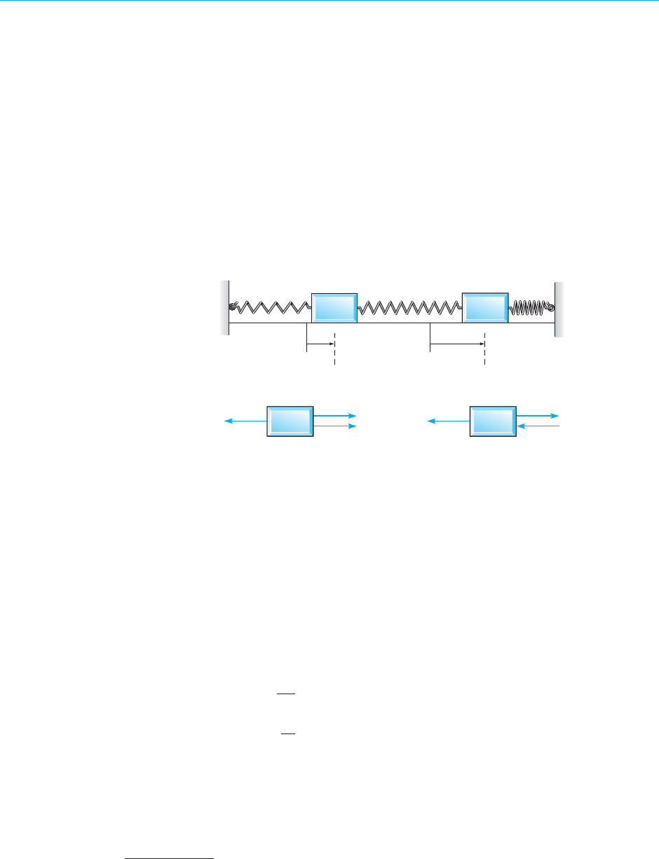
August 7, 2012 21:04 c07 Sheet number 7 Page number 365 cyan black
7.1 Introduction 365
16. Let x = x
1
(t), y = y
1
(t) and x = x
2
(t), y = y
2
(t) be any two solutions of the linear
nonhomogeneous system
x
′
= p
11
(t)x + p
12
(t)y + g
1
(t),
y
′
= p
21
(t)x + p
22
(t)y + g
2
(t).
Show that x = x
1
(t) − x
2
(t), y = y
1
(t) − y
2
(t) is a solution of the corresponding homoge-
neous system.
17. Equations (1) can be derived by drawing a free-body diagram showing the forces acting
on each mass. Figure 7.1.3a shows the situation when the displacements x
1
and x
2
of the
two masses are both positive (to the right) and x
2
> x
1
.Then springs 1 and 2 are elongated
and spring 3 is compressed, giving rise to forces as shown in Figure 7.1.3b. Use Newton’s
law (F = ma) to derive Eqs. (1).
k
1
k
2
x
1
x
2
k
3
(a)
m
2
m
1
F
1
(t)
k
1
x
1
k
2
(x
2
– x
1
)
k
2
(x
2
– x
1
) k
3
x
2
F
2
(t)
m
1
m
2
(b)
FIGURE 7.1.3 (a) The displacements x
1
and x
2
are both positive.
(b) The free-body diagram for the spring–mass system.
18. Transform the system (1) into a system of first order equations by letting y
1
= x
1
, y
2
= x
2
,
y
3
= x
′
1
, and y
4
= x
′
2
.
Electric Circuits. The theory of electric circuits, such as that shown in Figure 7.1.2, consisting
of inductors, resistors, and capacitors, is based on Kirchhoff’s laws: (1) The net flow of current
into each node (or junction) is zero, and (2) the net voltage drop around each closed loop
is zero. In addition to Kirchhoff’s laws, we also have the relation between the current I in
amperes through each circuit element and the voltage drop V in volts across the element:
V = RI, R = resistance in ohms;
C
dV
dt
= I, C = capacitance in farads
1
;
L
dI
dt
= V, L = inductance in henrys.
Kirchhoff’s laws and the current–voltage relation for each circuit element provide a system of
algebraic and differential equations from which the voltage and current throughout the circuit
can be determined. Problems 19 through 21 illustrate the procedure just described.
1
Actual capacitors typically have capacitances measured in microfarads. We use farad as the unit for
numerical convenience.

August 7, 2012 21:04 c07 Sheet number 8 Page number 366 cyan black
366 Chapter 7. Systems of First Order Linear Equations
19. Consider the circuit shown in Figure 7.1.2. Let I
1
, I
2
, and I
3
be the currents through the
capacitor, resistor, and inductor, respectively. Likewise, let V
1
, V
2
, and V
3
be the corre-
sponding voltage drops. The arrows denote the arbitrarily chosen directions in which
currents and voltage drops will be taken to be positive.
(a) Applying Kirchhoff’s second law to the upper loop in the circuit, show that
V
1
− V
2
= 0. (i)
In a similar way, show that
V
2
− V
3
= 0. (ii)
(b) Applying Kirchhoff’s first law to either node in the circuit, show that
I
1
+ I
2
+ I
3
= 0. (iii)
(c) Use the current–voltage relation through each element in the circuit to obtain the
equations
CV
′
1
= I
1
, V
2
= RI
2
, LI
′
3
= V
3
. (iv)
(d) Eliminate V
2
, V
3
, I
1
, and I
2
among Eqs. (i) through (iv) to obtain
CV
′
1
=−I
3
−
V
1
R
, LI
′
3
= V
1
. (v)
Observe that if we omit the subscripts in Eqs. (v), then we have the system (2) of this
section.
20. Consider the circuit shown in Figure 7.1.4. Use the method outlined in Problem 19 to show
that the current I through the inductor and the voltage V across the capacitor satisfy the
system of differential equations
dI
dt
=−I − V,
dV
dt
= 2I − V.
R = 1 ohm
R = 2 ohms
L = 1 henry
C = farad
1
2
FIGURE 7.1.4 The circuit in Problem 20.

August 7, 2012 21:04 c07 Sheet number 9 Page number 367 cyan black
7.1 Introduction 367
21. Consider the circuit shown in Figure 7.1.5. Use the method outlined in Problem 19 to show
that the current I through the inductor and the voltage V across the capacitor satisfy the
system of differential equations
L
dI
dt
=−R
1
I − V, C
dV
dt
= I −
V
R
2
.
C
L
R
2
R
1
FIGURE 7.1.5 The circuit in Problem 21.
22. Consider the two interconnected tanks shown in Figure 7.1.6. Tank 1 initially contains
30 gal of water and 25 oz of salt, and Tank 2 initially contains 20 gal of water and 15 oz
of salt. Water containing 1 oz/gal of salt flows into Tank 1 at a rate of 1.5 gal/min. The
mixture flows fromTank 1 to Tank 2 at a rate of 3 gal/min.Water containing 3 oz/gal of salt
also flows into Tank 2 at a rate of 1 gal/min (from the outside). The mixture drains from
Tank 2 at a rate of 4 gal/min, of which some flows back into Tank 1 at a rate of 1.5 gal/min,
while the remainder leaves the system.
(a) Let Q
1
(t) and Q
2
(t), respectively, be the amount of salt in each tank at time t. Write
down differential equations and initial conditions that model the flow process. Observe
that the system of differential equations is nonhomogeneous.
(b) Find the values of Q
1
and Q
2
for which the system is in equilibrium—that is, does not
change with time. Let Q
E
1
and Q
E
2
be the equilibrium values. Can you predict which tank
will approach its equilibrium state more rapidly?
(c) Let x
1
= Q
1
(t) − Q
E
1
and x
2
= Q
2
(t) − Q
E
2
. Determine an initial value problem for x
1
and x
2
. Observe that the system of equations for x
1
and x
2
is homogeneous.
1.5 gal/min
1 gal/min
3 gal/min
3 oz/gal
2 knaT1 knaT
Q
1
(t) oz salt
30 gal water
Q
2
(t) oz salt
20 gal water
2.5 gal/min
1 oz/gal
1.5 gal/min
FIGURE 7.1.6 Two interconnected tanks (Problem 22).

August 7, 2012 21:04 c07 Sheet number 10 Page number 368 cyan black
368 Chapter 7. Systems of First Order Linear Equations
23. Consider two interconnected tanks similar to those in Figure 7.1.6. Initially,Tank 1 contains
60 gal of water and Q
0
1
oz of salt, and Tank 2 contains 100 gal of water and Q
0
2
oz of salt.
Water containing q
1
oz/gal of salt flows into Tank 1 at a rate of 3 gal/min. The mixture
in Tank 1 flows out at a rate of 4 gal/min, of which half flows into Tank 2, while the
remainder leaves the system.Water containing q
2
oz/gal of salt also flows intoTank 2 from
the outside at the rate of 1 gal/min. The mixture in Tank 2 leaves it at a rate of 3 gal/min, of
which some flows back into Tank 1 at a rate of 1 gal/min, while the rest leaves the system.
(a) Draw a diagram that depicts the flow process described above. Let Q
1
(t) and Q
2
(t),
respectively,be the amount of salt in each tank at time t. Write down differential equations
and initial conditions for Q
1
and Q
2
that model the flow process.
(b) Find the equilibrium values Q
E
1
and Q
E
2
in terms of the concentrations q
1
and q
2
.
(c) Is it possible (by adjusting q
1
and q
2
) to obtain Q
E
1
= 60 and Q
E
2
= 50 as anequilibrium
state?
(d) Describe which equilibrium states are possible for this system for various values of q
1
and q
2
.
7.2 Review of Matrices
For both theoretical and computational reasons, it is advisable to bring some of the
results of matrix algebra
2
to bear on the initial value problem for a system of linear
differential equations. For reference purposes, this section and the next are devoted
to a brief summary of the facts that will be needed later. More details can be found
in any elementary book on linear algebra. We assume, however, that you are familiar
with determinants and how to evaluate them.
We designate matrices by boldfaced capitals A, B, C, ..., occasionally using bold-
faced Greek capitals #, $, ....A matrix A consists of a rectangular array of numbers,
or elements, arranged in m rows and n columns—that is,
A =
⎛
⎜
⎜
⎜
⎝
a
11
a
12
··· a
1n
a
21
a
22
··· a
2n
.
.
.
.
.
.
.
.
.
a
m1
a
m2
··· a
mn
⎞
⎟
⎟
⎟
⎠
. (1)
We speak of A as an m × n matrix. Although later in the chapter we will often assume
that the elements of certain matrices are real numbers, in this section we assume that
2
The properties of matrices were first extensively explored in 1858 in a paper by the English algebraist
Arthur Cayley (1821–1895),although the word“matrix”was introduced by his good friend James Sylvester
(1814–1897) in 1850. Cayley did some of his best mathematical work while practicing law from 1849 to
1863; he then became professor of mathematics at Cambridge, a position he held for the rest of his life.
After Cayley’s groundbreaking work,the development of matrix theory proceeded rapidly,with significant
contributions by Charles Hermite, Georg Frobenius, and Camille Jordan, among others.

August 7, 2012 21:04 c07 Sheet number 11 Page number 369 cyan black
7.2 Review of Matrices 369
the elements of matrices may be complex numbers. The element lying in the ith row
and jth column is designated by a
ij
, the first subscript identifying its row and the
second its column. Sometimes the notation (a
ij
) is used to denote the matrix whose
generic element is a
ij
.
Associated with each matrix A is the matrix A
T
, which is known as the transpose
of A and is obtained from A by interchanging the rows and columns of A.Thus,if
A = (a
ij
), then A
T
= (a
ji
). Also, we will denote by a
ij
the complex conjugate of a
ij
,
and by
A the matrix obtained from A by replacing each element a
ij
by its conjugate
a
ij
. The matrix A is called the conjugate of A. It will also be necessary to consider
the transpose of the conjugate matrix
A
T
. This matrix is called the adjoint of A and
will be denoted by A
∗
.
For example, let
A =
#
32− i
4 + 3i −5 + 2i
$
.
Then
A
T
=
#
34+ 3i
2 − i −5 + 2i
$
, A =
#
32+ i
4 − 3i −5 − 2i
$
,
A
∗
=
#
34− 3i
2 + i −5 − 2i
$
.
We are particularly interested in two somewhat special kinds of matrices: square
matrices, which have the same number of rows and columns—that is, m = n; and
vectors (or column vectors), which can be thought of as n × 1 matrices, or matri-
ces having only one column. Square matrices having n rows and n columns are
said to be of order n. We denote (column) vectors by boldfaced lowercase letters:
x, y, ξ, η, ....The transpose x
T
of an n × 1 column vector is a 1 × n row vector—that
is, the matrix consisting of one row whose elements are the same as the elements in
the corresponding positions of x.
Prop ert ie s of Mat ri ces .
1. Equality. Two m × n matrices A and B are said to be equal if all corresponding
elements are equal—that is, if a
ij
= b
ij
for each i and j.
2. Zero. The symbol 0 will be used to denote the matrix (or vector) each of whose
elements is zero.
3. Addition. The sum of two m × n matrices A and B is defined as the matrix
obtained by adding corresponding elements:
A + B = (a
ij
) + (b
ij
) = (a
ij
+ b
ij
). (2)

August 7, 2012 21:04 c07 Sheet number 12 Page number 370 cyan black
370 Chapter 7. Systems of First Order Linear Equations
With this definition, it follows that matrix addition is commutative and associative,
so that
A + B = B +A, A + (B + C) = (A + B) + C. (3)
4. Multiplication by a Number. The product of a matrix A by a real or complex
number α is defined as follows:
αA = α(a
ij
) = (αa
ij
); (4)
that is, each element of A is multiplied by α. The distributive laws
α(A + B) = αA + αB, (α + β)A = αA + βA (5)
are satisfied for this type of multiplication. In particular, the negative of A, denoted
by −A, is defined by
−A = (−1)A. (6)
5. Subtraction. The difference A − B of two m × n matrices is defined by
A − B = A + (−B). (7)
Thus
A − B = (a
ij
) − (b
ij
) = (a
ij
− b
ij
), (8)
which is similar to Eq. (2).
6. Multiplication. The product AB of two matrices is defined whenever the num-
ber of columns in the first factor is the same as the number of rows in the second.
If A and B are m × n and n × r matrices, respectively, then the product C = AB is an
m × r matrix. The element in the ith row and jth column of C is found by multiplying
each element of the ith row of A by the corresponding element of the jth column of
B and then adding the resulting products. In symbols,
c
ij
=
n
4
k=1
a
ik
b
kj
. (9)
By direct calculation, it can be shown that matrix multiplication satisfies the
associative law
(AB)C = A(BC) (10)
and the distributive law
A(B + C) = AB +AC. (11)
However, in general, matrix multiplication is not commutative. For both products
AB and BA to exist and to be of the same size, it is necessary that A and B be square
matrices of the same order. Even in that case the two products are usually unequal,
so that, in general,
AB ̸= BA. (12)

August 7, 2012 21:04 c07 Sheet number 13 Page number 371 cyan black
7.2 Review of Matrices 371
EXAMPLE
1
To illustrate the multiplication of matrices, and also the fact that matrix multiplication is not
necessarily commutative, consider the matrices
A =
⎛
⎜
⎝
1 −21
02−1
211
⎞
⎟
⎠
, B =
⎛
⎜
⎝
21−1
1 −10
2 −11
⎞
⎟
⎠
.
From the definition of multiplication given in Eq. (9), we have
AB =
⎛
⎜
⎝
2 − 2 + 21+ 2 − 1 −1 + 0 + 1
0 + 2 − 20− 2 + 10+ 0 − 1
4 + 1 + 22− 1 − 1 −2 + 0 + 1
⎞
⎟
⎠
=
⎛
⎜
⎝
220
0 −1 −1
70−1
⎞
⎟
⎠
.
Similarly
,
we find that
BA =
⎛
⎜
⎝
0 −30
1 −42
4 −54
⎞
⎟
⎠
.
Clearly, AB ̸= BA.
7. Multiplication of Vectors. There are several ways of forming a product of two
vectors x and y, each with n components. One is a direct extension to n dimensions
of the familiar dot product from physics and calculus; we denote it by x
T
y and write
x
T
y =
n
4
i=1
x
i
y
i
. (13)
The result of Eq. (13) isa realor complex number,and it follows directly fromEq. (13)
that
x
T
y = y
T
x, x
T
(y + z) = x
T
y + x
T
z, (αx)
T
y = α(x
T
y) = x
T
(αy). (14)
There is another vector product that is also defined for any two vectors having the
same number of components. This product, denoted by (x, y), is called the scalar or
inner product and is defined by
(x, y) =
n
4
i=1
x
i
y
i
. (15)
The scalar product is also a real or complex number, and by comparing Eqs. (13) and
(15), we see that
(x, y) = x
T
y. (16)
Thus,if all the elements of y are real,then the two products (13) and (15) are identical.
From Eq. (15) it follows that
(x, y) =
(y, x), (x, y + z) = (x, y) + (x, z),
(17)
(αx, y) = α(x, y), (x, αy) =
α(x, y).

August 7, 2012 21:04 c07 Sheet number 14 Page number 372 cyan black
372 Chapter 7. Systems of First Order Linear Equations
Note that even if the vector x has elements with nonzero imaginary parts,the scalar
product of x with itself yields a nonnegative real number
(x, x) =
n
4
i=1
x
i
x
i
=
n
4
i=1
|x
i
|
2
. (18)
The nonnegative quantity (x, x)
1/2
, often denoted by ∥x∥, is called the length, or
magnitude,ofx.If(x, y) = 0, then the two vectors x and y are said to be orthogonal.
For example, the unit vectors i, j, k of three-dimensional vector geometry form an
orthogonal set. On the other hand, if some of the elements of x are not real, then the
product
x
T
x =
n
4
i=1
x
2
i
(19)
may not be a real number.
For example, let
x =
⎛
⎜
⎝
i
−2
1 + i
⎞
⎟
⎠
, y =
⎛
⎜
⎝
2 − i
i
3
⎞
⎟
⎠
.
Then
x
T
y = (i)(2 − i) + (−2)(i) + (1 + i)(3) = 4 + 3i,
(x, y) = (i)(2 + i) + (−2)(−i) + (1 + i )(3) = 2 + 7i,
x
T
x = (i)
2
+ (−2)
2
+ (1 + i)
2
= 3 + 2i,
(x, x) = (i)(−i ) + (−2)(−2) + (1 + i)(1 − i) = 7.
8. Identity. The multiplicative identity, or simply the identity matrix I, is given by
I =
⎛
⎜
⎜
⎜
⎝
10··· 0
01··· 0
.
.
.
.
.
.
.
.
.
00··· 1
⎞
⎟
⎟
⎟
⎠
. (20)
From the definition of matrix multiplication, we have
AI = IA = A (21)
for any (square) matrix A. Hence the commutative law does hold for square matrices
if one of the matrices is the identity.
9. Inverse. The square matrix A is said to be nonsingular or invertible if there
is another matrix B such that AB = I and BA = I
, where I is the identity. If there is
such
a B, it can be shown that there is only one. It is called the multiplicative inverse,
or simply the inverse, of A, and we write B = A
−1
. Then
AA
−1
= A
−1
A = I. (22)
Matrices that do not have an inverse are called singular or noninvertible.
There are various ways to compute A
−1
from A, assuming that it exists. One way
involves the use of determinants. Associated with each element a
ij
of a given matrix

August 7, 2012 21:04 c07 Sheet number 15 Page number 373 cyan black
7.2 Review of Matrices 373
is the minor M
ij
, which is the determinant of the matrix obtained by deleting the
ith row and jth column of the original matrix—that is, the row and column con-
taining a
ij
. Also associated with each element a
ij
is the cofactor C
ij
defined by the
equation
C
ij
= (−1)
i+j
M
ij
. (23)
If B = A
−1
, then it can be shown that the general element b
ij
is given by
b
ij
=
C
ji
detA
. (24)
Although Eq. (24) is not an efficient way
3
to calculate A
−1
, it does suggest a con-
dition that A must satisfy for it to have an inverse. In fact, the condition is both
necessary and sufficient: A is nonsingular if and only if det A ̸= 0. If detA = 0, then
A is singular.
Another (and usually better) way to compute A
−1
is by means of elementary row
operations. There are three such operations:
1. Interchange of two rows.
2. Multiplication of a row by a nonzero scalar.
3. Addition of any multiple of one row to another row.
The transformation of a matrix by a sequence of elementary row operations is
referred to as row reduction or Gaussian
4
elimination. Any nonsingular matrix A
can be transformed into the identity I by a systematic sequence of these operations.
It is possible to show that if the same sequence of operations is then performed on I,it
is transformed into A
−1
. It is most efficient to perform the sequence of operations on
both matrices at the same time by forming the augmented matrix A |I. The following
example illustrates the calculation of an inverse matrix in this way.
EXAMPLE
2
Find the inverse of
A =
⎛
⎜
⎝
1 −1 −1
3 −12
223
⎞
⎟
⎠
.
3
For large n the number of multiplications required to evaluate A
−1
by Eq. (24) is proportional to n!. If we
use a more efficient method, such as the row reduction procedure described in this section, the number
of multiplications is proportional only to n
3
. Even for small values of n (such as n = 4), determinants are
not an economical tool in calculating inverses, and row reduction methods are preferred.
4
Carl Friedrich Gauss (1777–1855) was born in Brunswick (Germany) and spent most of his life as pro-
fessor of astronomy and director of the Observatory at the University of Göttingen. Gauss made major
contributions to many areas of mathematics, including number theory, algebra, non-Euclidean and dif-
ferential geometry, and analysis, as well as to more applied fields such as geodesy, statistics, and celestial
mechanics. He is generally considered to be among the half-dozen best mathematicians of all time.

August 7, 2012 21:04 c07 Sheet number 16 Page number 374 cyan black
374 Chapter 7. Systems of First Order Linear Equations
We begin by forming the augmented matrix A |I:
A |I =
⎛
⎜
⎝
1 −1 −1
100
3 −12
010
223
001
⎞
⎟
⎠
.
The matrix A can be transformed into I by the following sequence of operations, and at the
same time, I is transformed into A
−1
. The result of each step appears below the statement.
(a) Obtain zeros in the off-diagonal positions in the first column by adding (−3) times the
first row to the second row and adding (−2) times the first row to the third row.
⎛
⎜
⎝
1 −1 −1
100
025
−310
045
−201
⎞
⎟
⎠
(b) Obtain a 1 in the diagonal position in the second column by multiplying the second row
by
1
2
.
⎛
⎜
⎝
1 −1 −1
100
01
5
2
−
3
2
1
2
0
045
−201
⎞
⎟
⎠
(c) Obtain zeros in the off-diagonal positions in the second column by adding the second row
to the first row and adding (−4) times the second row to the third row.
⎛
⎜
⎝
10
3
2
−
1
2
1
2
0
01
5
2
−
3
2
1
2
0
00−5
4 −21
⎞
⎟
⎠
(d) Obtaina1inthediagonal position in the third column by multiplying the third row by
(−
1
5
).
⎛
⎜
⎝
10
3
2
−
1
2
1
2
0
01
5
2
−
3
2
1
2
0
001
−
4
5
2
5
−
1
5
⎞
⎟
⎠
(e) Obtain zeros in the off-diagonal positions in the third column by adding (−
3
2
) times the
third row to the first row and adding (−
5
2
) times the third row to the second row.
⎛
⎜
⎝
100
7
10
−
1
10
3
10
010
1
2
−
1
2
1
2
001−
4
5
2
5
−
1
5
⎞
⎟
⎠
The last of these matrices is I |A
−1
, a fact that can be verified by direct multiplication with
the original matrix A.
This example was made slightly simpler by the fact that the given matrix A had a 1
in the upper left corner (a
11
= 1). If this is not the case,then the first step is to produce
a 1 there by multiplying the first row by 1/a
11
, as long as a
11
̸= 0. If a
11
= 0, then the
first row must be interchanged with some other row to bring a nonzero element
into the upper left position before proceeding. If this cannot be done, because every
element in the first column is zero, then the matrix has no inverse and is singular.

August 7, 2012 21:04 c07 Sheet number 17 Page number 375 cyan black
7.2 Review of Matrices 375
A similar situation may occur at later stages of the process as well, and the remedy
is the same: interchange the given row with a lower row so as to bring a nonzero
element to the desired diagonal location. If this cannot be done, then the original
matrix is singular.
Matrix Functions. We sometimes need to consider vectors or matrices whose elements
are functions of a real variable t. We write
x(t) =
⎛
⎜
⎝
x
1
(t)
.
.
.
x
n
(t)
⎞
⎟
⎠
, A(t) =
⎛
⎜
⎝
a
11
(t) ··· a
1n
(t)
.
.
.
.
.
.
a
m1
(t) ··· a
mn
(t)
⎞
⎟
⎠
, (25)
respectively.
The matrix A(t) is said to be continuous at t = t
0
or on an interval α<t <βif each
element of A is a continuous function at the given point or on the given interval.
Similarly,A(t) is said to be differentiable if each of its elements is differentiable, and
its derivative dA/dt is defined by
dA
dt
=
'
da
ij
dt
(
; (26)
that is, each element of dA/dt is the derivative of the corresponding element of A.
In the same way, the integral of a matrix function is defined as
"
b
a
A(t) dt =
'
"
b
a
a
ij
(t) dt
(
. (27)
For example, if
A(t) =
'
sin tt
1 cos t
(
,
then
A
′
(t) =
'
cos t 1
0 −sin t
(
,
"
π
0
A(t) dt =
'
2 π
2
/2
π 0
(
.
Many of the rules of elementary calculus extend easily to matrix functions; in partic-
ular,
d
dt
(CA) = C
dA
dt
, where C is a constant matrix; (28)
d
dt
(A + B) =
dA
dt
+
d B
dt
; (29)
d
dt
(AB) = A
d B
dt
+
dA
dt
B. (30)
In Eqs. (28) and (30), care must be taken in each term to avoid interchanging the
order of multiplication. The definitions expressed by Eqs. (26) and (27) also apply as
special cases to vectors.
To conclude this section:some important operations on matrices are accomplished
by applyingthe operation separately to each element ofthe matrix. Examples include

August 7, 2012 21:04 c07 Sheet number 18 Page number 376 cyan black
376 Chapter 7. Systems of First Order Linear Equations
multiplication by a number,differentiation, and integration. However,this is not true
of many other operations. For instance, the square of a matrix is not calculated by
squaring each of its elements.
PROBLEMS
1. If A =
⎛
⎜
⎝
1 −20
32−1
−213
⎞
⎟
⎠
and B =
⎛
⎜
⎝
4 −23
−150
612
⎞
⎟
⎠
, find
(a) 2A + B (b) A − 4B
(c) AB (d) BA
2. If A =
#
1 + i −1 + 2i
3 + 2i 2 − i
$
and B =
#
i 3
2 −2i
$
, find
(a) A −2B (b) 3A + B
(c) AB (d) BA
3. If A =
⎛
⎜
⎝
−212
10−3
2 −11
⎞
⎟
⎠
and B =
⎛
⎜
⎝
12
3
3 −
1 −1
−210
⎞
⎟
⎠
, find
(a) A
T
(b) B
T
(c) A
T
+ B
T
(d) (A + B)
T
4. If A =
#
3 − 2i 1 + i
2 − i −2 + 3i
$
, find
(a) A
T
(b) A (c) A
∗
5. If A =
⎛
⎜
⎝
32−1
2 −12
121
⎞
⎟
⎠
and B =
⎛
⎜
⎝
21−1
−233
102
⎞
⎟
⎠
, verify that 2(A + B) = 2A + 2B.
6. If A =
⎛
⎜
⎝
1 −20
32−1
−203
⎞
⎟
⎠
, B =
⎛
⎜
⎝
21−1
−233
102
⎞
⎟
⎠
, and C =
⎛
⎜
⎝
210
122
01−1
⎞
⎟
⎠
, verify that
(a) (AB)C = A(BC) (b) (A + B) + C = A + (B + C)
(c) A(B + C) = AB +AC
7.
Prove
each of the following laws of matrix algebra:
(a) A + B = B +A (b) A + (B + C) = (A + B) + C
(c) α(A + B) = αA + αB (d) (α + β)A = αA + βA
(e) A (BC) = (AB)C (f) A(B + C) = AB +AC
8. If x =
⎛
⎜
⎝
2
3i
1 − i
⎞
⎟
⎠
and y =
⎛
⎜
⎝
−1 + i
2
3 − i
⎞
⎟
⎠
,
find
(a) x
T
y (b) y
T
y
(c) (x, y) (d) (y, y)

August 7, 2012 21:04 c07 Sheet number 19 Page number 377 cyan black
7.2 Review of Matrices 377
9. If x =
⎛
⎜
⎝
1 − 2i
i
2
⎞
⎟
⎠
and y =
⎛
⎜
⎝
2
3 − i
1 + 2i
⎞
⎟
⎠
, show that
(a) x
T
y = y
T
x (b) (x,y) = (y, x)
In each of Problems 10 through 19, either compute the inverse of the given matrix, or else
show that it is singular.
10.
#
14
−23
$
11.
#
3 −1
62
$
12.
⎛
⎜
⎝
123
245
356
⎞
⎟
⎠
13.
⎛
⎜
⎝
11−1
2 −11
112
⎞
⎟
⎠
14.
⎛
⎜
⎝
121
−218
1 −2 −7
⎞
⎟
⎠
15.
⎛
⎜
⎝
210
021
002
⎞
⎟
⎠
16.
⎛
⎜
⎝
1 −1 −1
210
3 −21
⎞
⎟
⎠
17.
⎛
⎜
⎝
231
−121
4 −1 −1
⎞
⎟
⎠
18.
⎛
⎜
⎜
⎜
⎝
100−1
0 −110
−10
10
01−
11
⎞
⎟
⎟
⎟
⎠
19.
⎛
⎜
⎜
⎜
⎝
1 −120
−12−42
1013
−220−1
⎞
⎟
⎟
⎟
⎠
20. IfA is a square matrix,and if there are two matrices B and C such that AB = I and CA = I,
show that B = C. Thus, if a matrix has an inverse, it can have only one.
21. If A(t) =
⎛
⎜
⎝
e
t
2e
−t
e
2t
2e
t
e
−t
−e
2t
−e
t
3e
−t
2e
2t
⎞
⎟
⎠
and B(t) =
⎛
⎜
⎝
2e
t
e
−t
3e
2t
−e
t
2e
−t
e
2t
3e
t
−e
−t
−e
2t
⎞
⎟
⎠
, find
(a) A + 3B (b) AB
(c) dA/dt (d)
"
1
0
A(t) dt
In each of Problems 22 through 24, verify that the given vector satisfies the given differential
equation.
22. x
′
=
#
3 −2
2 −2
$
x, x =
#
4
2
$
e
2t
23. x
′
=
#
2 −1
3 −2
$
x +
#
1
−1
$
e
t
, x =
#
1
0
$
e
t
+ 2
#
1
1
$
te
t

August 7, 2012 21:04 c07 Sheet number 20 Page number 378 cyan black
378 Chapter 7. Systems of First Order Linear Equations
24. x
′
=
⎛
⎜
⎝
111
21−1
0 −11
⎞
⎟
⎠
x, x =
⎛
⎜
⎝
6
−8
−4
⎞
⎟
⎠
e
−t
+ 2
⎛
⎜
⎝
0
1
−1
⎞
⎟
⎠
e
2t
In each of Problems 25 and 26, verify that the given matrix satisfies the given differential
equation.
25. $
′
=
#
11
4 −2
$
$, $(t) =
#
e
−3t
e
2t
−4e
−3t
e
2t
$
26. $
′
=
⎛
⎜
⎝
1 −14
32−1
21−1
⎞
⎟
⎠
$, $(t) =
⎛
⎜
⎝
e
t
e
−2t
e
3t
−4e
t
−e
−2t
2e
3t
−e
t
−e
−2t
e
3t
⎞
⎟
⎠
7.3 Systems of Linear Algebraic Equations; Linear Independence,
Eigenvalues, Eigenvectors
In this section we review some results from linear algebra that are important for the
solution of systems of linear differential equations. Some of these results are easily
proved and others are not;since we are interested simply in summarizing some useful
information in compact form, we give no indication of proofs in either case. All the
results in this section depend on some basic facts about the solution of systems of
linear algebraic equations.
Systems of Linear Algebraic Equations. A set ofn simultaneouslinear algebraic equations
in n variables
a
11
x
1
+ a
12
x
2
+···+a
1n
x
n
= b
1
,
.
.
. (1)
a
n1
x
1
+ a
n2
x
2
+···+a
nn
x
n
= b
n
can be written as
Ax = b, (2)
where the n × n matrix A and the vector b are given, and the components of x are
to be determined. If b = 0, the system is said to be homogeneous; otherwise, it is
nonhomogeneous.
If the coefficient matrix A is nonsingular—that is, if detA is not zero—then there
is a unique solution of the system (2). Since A is nonsingular, A
−1
exists, and the
solution can be found by multiplying each side of Eq. (2) on the left by A
−1
; thus
x = A
−1
b. (3)
In particular, the homogeneous problem Ax = 0, corresponding to b = 0 in Eq. (2),
has only the trivial solution x = 0.

August 7, 2012 21:04 c07 Sheet number 21 Page number 379 cyan black
7.3 Systems of Linear Equations; Linear Independence, Eigenvalues, Eigenvectors 379
On the other hand, if A is singular—that is, if detA is zero—then solutions of
Eq. (2) either do not exist, or do exist but are not unique. Since A is singular, A
−1
does not exist, so Eq. (3) is no longer valid. The homogeneous system
Ax = 0 (4)
has (infinitely many) nonzero solutions in addition to the trivial solution. The situ-
ation for the nonhomogeneous system (2) is more complicated. This system has no
solution unless the vector b satisfies a certain further condition.This condition is that
(b, y) = 0, (5)
for all vectors y satisfying A
∗
y = 0, where A
∗
is the adjoint of A. If condition (5) is
met, then the system (2) has (infinitely many) solutions. These solutions are of the
form
x = x
(0)
+ ξ, (6)
where x
(0)
is a particular solution of Eq. (2), and ξ is the most general solution of the
homogeneous system (4). Note the resemblance between Eq. (6) and the solution of
a nonhomogeneous linear differential equation. The proofs of some of the preceding
statements are outlined in Problems 26 through 30.
The results in the preceding paragraph are important as a means of classifying the
solutions of linear systems. However,for solving particular systems,it is generally best
to use row reduction to transform the system into a much simpler one from which
the solution(s), if there are any, can be written down easily. To do this efficiently, we
can form the augmented matrix
A |b =
⎛
⎜
⎝
a
11
··· a
1n
b
1
.
.
.
.
.
.
.
.
.
a
n1
··· a
nn
b
n
⎞
⎟
⎠
(7)
by adjoining the vector b to the coefficient matrix A as an additional column. The
vertical line replaces the equals sign and is said to partition the augmented matrix.
We now perform row operations on the augmented matrix so as to transform A into
an upper triangular matrix—that is,a matrix whose elements belowthe maindiagonal
are all zero. Once this is done, it is easy to see whether the system has solutions, and
to find them if it does. Observe that elementary row operations on the augmented
matrix (7) correspond to legitimate operations on the equations in the system (1).
The following examples illustrate the process.
EXAMPLE
1
Solve the system of equations
x
1
− 2x
2
+ 3x
3
= 7,
−x
1
+ x
2
− 2x
3
=−5, (8)
2x
1
− x
2
− x
3
= 4.

August 7, 2012 21:04 c07 Sheet number 22 Page number 380 cyan black
380 Chapter 7. Systems of First Order Linear Equations
The augmented matrix for the system (8) is
⎛
⎜
⎝
1 −23
7
−11−2
−5
2 −1 −1
4
⎞
⎟
⎠
. (9)
We now perform row operations on the matrix (9) with a view to introducing zeros in the
lower left part of the matrix. Each step is described and the result recorded below.
(a) Add the first row to the second row, and add (−2) times the first row to the third row.
⎛
⎜
⎝
1 −23
7
0 −11
2
03−7
−10
⎞
⎟
⎠
(b) Multiply the second row by −1.
⎛
⎜
⎝
1 −23
7
01−1
−2
03−7
−10
⎞
⎟
⎠
(c) Add (−3) times the second row to the third row.
⎛
⎜
⎝
1 −23
7
01−1
−2
00−4
−4
⎞
⎟
⎠
(d) Divide the third row by −4.
⎛
⎜
⎝
1 −23
7
01−1
−2
001
1
⎞
⎟
⎠
The matrix obtained in this manner corresponds to the system of equations
x
1
− 2x
2
+ 3x
3
= 7,
x
2
− x
3
=−2, (10)
x
3
= 1,
which is equivalent to the original system (8). Note that the coefficients in Eqs. (10) form
a triangular matrix. From the last of Eqs. (10) we have x
3
= 1, from the second equation
x
2
=−2 + x
3
=−1, and from the first equation x
1
= 7 + 2x
2
− 3x
3
= 2. Thus we obtain
x =
⎛
⎜
⎝
2
−1
1
⎞
⎟
⎠
,
which is the solution of the given system (8). Incidentally, since the solution is unique, we
conclude that the coefficient matrix is nonsingular.

August 7, 2012 21:04 c07 Sheet number 23 Page number 381 cyan black
7.3 Systems of Linear Equations; Linear Independence, Eigenvalues, Eigenvectors 381
EXAMPLE
2
Discuss solutions of the system
x
1
− 2x
2
+ 3x
3
= b
1
,
−x
1
+ x
2
− 2x
3
= b
2
, (11)
2x
1
− x
2
+ 3x
3
= b
3
for various values of b
1
, b
2
, and b
3
.
Observe that the coefficientsin thesystem (11)are the same as those in thesystem (8)except
for the coefficient of x
3
in the third equation. The augmented matrix for the system (11) is
⎛
⎜
⎝
1 −23
b
1
−11−2 b
2
2 −13b
3
⎞
⎟
⎠
. (12)
By performing steps (a), (b), and (c) as in Example 1, we transform the matrix (12) into
⎛
⎜
⎝
1 −23
b
1
01−1 −b
1
− b
2
000b
1
+ 3b
2
+ b
3
⎞
⎟
⎠
. (13)
The equation corresponding to the third row of the matrix (13) is
b
1
+ 3b
2
+ b
3
= 0; (14)
thus the system (11) has no solution unless the condition (14) is satisfied by b
1
, b
2
, and b
3
.Itis
possible to show that this condition is just Eq. (5) for the system (11).
Let us now assume that b
1
= 2,b
2
= 1, and b
3
=−5,in which case Eq. (14) is satisfied. Then
the first two rows of the matrix (13) correspond to the equations
x
1
− 2x
2
+ 3x
3
= 2,
(15)
x
2
− x
3
=−3.
To solve the system (15), we can choose one of the unknowns arbitrarily and then solve for
the other two. If we let x
3
= α, where α is arbitrary, it then follows that
x
2
= α − 3,
x
1
= 2(α − 3) − 3α + 2 =−α − 4.
If we write the solution in vector notation, we have
x =
⎛
⎜
⎝
−α − 4
α − 3
α
⎞
⎟
⎠
= α
⎛
⎜
⎝
−1
1
1
⎞
⎟
⎠
+
⎛
⎜
⎝
−4
−3
0
⎞
⎟
⎠
. (16)
It is easy to verify that the second term on the right side of Eq. (16) is a solution of the nonho-
mogeneous system (11) and that the first term is the most general solution of the homogeneous
system corresponding to (11).
Row reduction is also useful in solving homogeneous systems and systems in which
the number of equations is different from the number of unknowns.

August 7, 2012 21:04 c07 Sheet number 24 Page number 382 cyan black
382 Chapter 7. Systems of First Order Linear Equations
Linear Dependence and Independence. A set of k vectors x
(1)
, ..., x
(k)
is said to be linearly
dependent if there exists a set of real or complex numbers c
1
, ..., c
k
, at least one of
which is nonzero, such that
c
1
x
(1)
+···+c
k
x
(k)
= 0. (17)
In other words, x
(1)
, ..., x
(k)
are linearly dependent if there is a linear relation among
them. On the other hand, if the only set c
1
, ..., c
k
for which Eq. (17) is satisfied is
c
1
= c
2
=···=c
k
= 0, then x
(1)
, ..., x
(k)
are said to be linearly independent.
Consider now a set of n vectors, each of which has n components. Let x
ij
= x
(j )
i
be
the ith component of the vector x
(j )
,and let X = (x
ij
).Then Eq. (17) can be written as
⎛
⎜
⎝
x
(1)
1
c
1
+···+x
(n)
1
c
n
.
.
.
.
.
.
x
(1)
n
c
1
+···+x
(n)
n
c
n
⎞
⎟
⎠
=
⎛
⎜
⎝
x
11
c
1
+···+x
1n
c
n
.
.
.
.
.
.
x
n1
c
1
+···+x
nn
c
n
⎞
⎟
⎠
= 0,
or, equivalently,
Xc = 0. (18)
If det X ̸= 0, then the only solution of Eq. (18) is c = 0, but if det X = 0, there are
nonzero solutions. Thus the set of vectors x
(1)
, ..., x
(n)
is linearly independent if and
only if det X ̸= 0.
EXAMPLE
3
Determine whether the vectors
x
(1)
=
⎛
⎜
⎝
1
2
−1
⎞
⎟
⎠
, x
(2)
=
⎛
⎜
⎝
2
1
3
⎞
⎟
⎠
, x
(3)
=
⎛
⎜
⎝
−4
1
−11
⎞
⎟
⎠
(19)
are linearly independent or linearly dependent. If they are linearly dependent, find a linear
relation among them.
To determine whether x
(1)
, x
(2)
, and x
(3)
are linearly dependent, we seek constants c
1
, c
2
, and
c
3
such that
c
1
x
(1)
+ c
2
x
(2)
+ c
3
x
(3)
= 0. (20)
Equation (20) can also be written in the form
⎛
⎜
⎝
12−4
21 1
−13−11
⎞
⎟
⎠
⎛
⎜
⎝
c
1
c
2
c
3
⎞
⎟
⎠
=
⎛
⎜
⎝
0
0
0
⎞
⎟
⎠
(21)
and solved by means of elementary row operations starting from the augmented matrix
⎛
⎜
⎝
12−4
0
21 1
0
−13−11
0
⎞
⎟
⎠
. (22)
We proceed as in Examples 1 and 2.

August 7, 2012 21:04 c07 Sheet number 25 Page number 383 cyan black
7.3 Systems of Linear Equations; Linear Independence, Eigenvalues, Eigenvectors 383
(a) Add (−2) times the first row to the second row, and add the first row to the third row.
⎛
⎜
⎝
12−4
0
0 −39
0
05−15
0
⎞
⎟
⎠
(b) Divide the second row by −3; then add (−5) times the second row to the third row.
⎛
⎜
⎝
12−4
0
01−3
0
000
0
⎞
⎟
⎠
Thus we obtain the equivalent system
c
1
+ 2c
2
− 4c
3
= 0,
(23)
c
2
− 3c
3
= 0.
From the second of Eqs. (23) we have c
2
= 3c
3
, and then from the first we obtain
c
1
= 4c
3
− 2c
2
=−2c
3
. Thus we have solved for c
1
and c
2
in terms of c
3
, with the latter remain-
ing arbitrary. If we choose c
3
=−1 for convenience, then c
1
= 2 and c
2
=−3. In this case the
relation (20) becomes
2x
(1)
− 3x
(2)
− x
(3)
= 0,
and the given vectors are linearly dependent.
Alternatively, we can compute det(x
ij
), whose columns are the components of x
(1)
, x
(2)
, and
x
(3)
, respectively. Thus
det(x
ij
) =
3
3
3
3
3
3
12−4
21 1
−13−11
3
3
3
3
3
3
and direct calculation shows that it is zero. Hence x
(1)
, x
(2)
, and x
(3)
are linearly dependent.
However, if the coefficients c
1
, c
2
, and c
3
are required, we still need to solve Eq. (20) to find
them.
Frequently, it is useful to think of the columns (or rows) of a matrix A as vectors.
These column (or row) vectors are linearly independent if and only if detA ̸= 0.
Further, if C = AB, then it can be shown that det C = (det A)(det B). Therefore, if
the columns (or rows) of both A and B are linearly independent, then the columns
(or rows) of C are also linearly independent.
Now let us extend the concepts of linear dependence and independence to a set
of vector functions x
(1)
(t), ..., x
(k)
(t) defined on an interval α<t <β. The vectors
x
(1)
(t), ..., x
(k)
(t) are said to be linearly dependent on α<t <βif there exists a set
of constants c
1
, ..., c
k
, not all of which are zero, such that
c
1
x
(1)
(t) +···+c
k
x
(k)
(t) = 0 for all t in the interval.
Otherwise, x
(1)
(t), ..., x
(k)
(t) are said to be linearly independent. Note that if
x
(1)
(t), ..., x
(k)
(t) are linearly dependent on an interval, they are linearly dependent
at each point in the interval. However, if x
(1)
(t), ..., x
(k)
(t) are linearly independent
on an interval, they may or may not be linearly independent at each point; they may,

August 7, 2012 21:04 c07 Sheet number 26 Page number 384 cyan black
384 Chapter 7. Systems of First Order Linear Equations
in fact, be linearly dependent at each point, but with different sets of constants at
different points. See Problem 15 for an example.
Eigenvalues and Eigenvectors. The equation
Ax = y (24)
can be viewed as a linear transformation that maps (or transforms) a given vector x
into a new vector y. Vectors that are transformed into multiples of themselves are
important in many applications.
5
To find such vectors, we set y = λx, where λ is a
scalar proportionality factor, and seek solutions of the equation
Ax = λx, (25)
or
(A − λI)x = 0. (26)
The latter equation has nonzero solutions if and only if λ is chosen so that
det(A − λI) = 0. (27)
Equation (27) is a polynomial equation of degree n in λ and is called the characteristic
equation of the matrix A. Values of λ that satisfy Eq. (27) may be either real- or
complex-valued and are called eigenvalues of A. The nonzero solutions of Eq. (25)
or (26) that are obtained by using such a value of λ are called the eigenvectors
corresponding to that eigenvalue.
If A is a 2 × 2 matrix, then Eq. (26) is
'
a
11
− λ a
12
a
21
a
22
− λ
('
x
1
x
2
(
=
'
0
0
(
(28)
and Eq. (27) becomes
(a
11
− λ)(a
22
− λ) − a
12
a
21
= 0,
or
λ
2
− (a
11
+ a
22
)λ + a
11
a
22
− a
12
a
21
= 0. (29)
The following example illustrates how eigenvalues and eigenvectors are found.
EXAMPLE
4
Find the eigenvalues and eigenvectors of the matrix
A =
#
3 −1
4 −2
$
. (30)
The eigenvalues λ and eigenvectors x satisfy the equation (A − λI)x = 0, or
#
3 − λ −1
4 −2 − λ
$#
x
1
x
2
$
=
#
0
0
$
. (31)
5
For example, this problem is encountered in finding the principal axes of stress or strain in an elastic
body, and in finding the modes of free vibration in a conservative system with a finite number of degrees
of freedom.

August 7, 2012 21:04 c07 Sheet number 27 Page number 385 cyan black
7.3 Systems of Linear Equations; Linear Independence, Eigenvalues, Eigenvectors 385
The eigenvalues are the roots of the equation
det(A − λI) =
3
3
3
3
3
3 − λ −1
4 −2 − λ
3
3
3
3
3
= λ
2
− λ − 2 = (λ − 2)(λ + 1) = 0. (32)
Thus the eigenvalues are λ
1
= 2 and λ
2
=−1.
To find the eigenvectors, we return to Eq. (31) and replace λ by each of the eigenvalues in
turn. For λ = 2 we have
#
1 −1
4 −4
$#
x
1
x
2
$
=
#
0
0
$
. (33)
Hence each row of this vector equation leads to the condition x
1
− x
2
= 0, so x
1
and x
2
are
equal but their value is not determined. If x
1
= c, then x
2
= c also, and the eigenvector x
(1)
is
x
(1)
= c
#
1
1
$
, c ̸= 0. (34)
Thus there is an infinite family of eigenvectors,indexed by the arbitrary constant c,correspond-
ing to the eigenvalue λ
1
. We will choose a single member of this family as a representative of
the rest; in this example it seems simplest to let c = 1. Then, instead of Eq. (34), we write
x
(1)
=
#
1
1
$
(35)
and remember that any nonzero multiple of this vector is also an eigenvector. We say that x
(1)
is the eigenvector corresponding to the eigenvalue λ
1
= 2.
Now, setting λ =−1 in Eq. (31), we obtain
#
4 −1
4 −1
$#
x
1
x
2
$
=
#
0
0
$
. (36)
Again we obtain a single condition on x
1
and x
2
, namely, 4x
1
− x
2
= 0. Thus the eigenvector
corresponding to the eigenvalue λ
2
=−1 is
x
(2)
=
#
1
4
$
(37)
or any nonzero multiple of this vector.
As Example 4 illustrates, eigenvectors are determined only up to an arbitrary
nonzero multiplicative constant; if this constant is specified in some way, then the
eigenvectors are said to be normalized. In Example 4, we chose the constant c so
that the components of the eigenvectors would be small integers. However, any
other choice of c is equally valid, although perhaps less convenient. Sometimes it
is useful to normalize an eigenvector x by choosing the constant so that its length
∥x∥=(x, x)
1/2
= 1.
Since the characteristic equation (27) for an n × n matrix A is a polynomial equa-
tion of degree n in λ, each such matrix has n eigenvalues λ
1
, ..., λ
n
, some of which
may be repeated. If a given eigenvalue appears m times as a root of Eq. (27), then
that eigenvalue is said to have algebraic multiplicity m. Each eigenvalue has at least
one associated eigenvector,and an eigenvalue of algebraic multiplicity m may have q

August 7, 2012 21:04 c07 Sheet number 28 Page number 386 cyan black
386 Chapter 7. Systems of First Order Linear Equations
linearly independent eigenvectors. The integer q is called the geometric multiplicity
of the eigenvalue, and it is possible to show that
1 ≤ q ≤ m. (38)
Further, examples demonstrate that q may be any integer in this interval. If each
eigenvalue of A is simple (has algebraic multiplicity 1),then each eigenvalue also has
geometric multiplicity 1.
It is possible to show that if λ
1
and λ
2
are two eigenvalues of A and if λ
1
̸= λ
2
,then
their corresponding eigenvectors x
(1)
and x
(2)
are linearly independent (Problem 34).
This result extends to any set λ
1
, ..., λ
k
of distinct eigenvalues: their eigenvectors
x
(1)
, ..., x
(k)
are linearly independent. Thus, if each eigenvalue of an n × n matrix
is simple, then the n eigenvectors of A, one for each eigenvalue, are linearly inde-
pendent. On the other hand, if A has one or more repeated eigenvalues, then there
may be fewer than n linearly independent eigenvectors associated with A, since for a
repeated eigenvalue we may have q < m. As we will see in Section 7.8, this fact may
lead to complications later on in the solution of systems of differential equations.
EXAMPLE
5
Find the eigenvalues and eigenvectors of the matrix
A =
⎛
⎜
⎝
011
101
110
⎞
⎟
⎠
. (39)
The eigenvalues λ and eigenvectors x satisfy the equation (A − λI)x = 0, or
⎛
⎜
⎝
−λ 11
1 −λ 1
11−λ
⎞
⎟
⎠
⎛
⎜
⎝
x
1
x
2
x
3
⎞
⎟
⎠
=
⎛
⎜
⎝
0
0
0
⎞
⎟
⎠
. (40)
The eigenvalues are the roots of the equation
det(A − λI) =
3
3
3
3
3
3
3
−λ 11
1 −λ 1
11−λ
3
3
3
3
3
3
3
=−λ
3
+ 3λ + 2 = 0. (41)
The roots of Eq. (41) are λ
1
= 2, λ
2
=−1, and λ
3
=−1. Thus 2 is a simple eigenvalue, and −1
is an eigenvalue of algebraic multiplicity 2, or a double eigenvalue.
To find the eigenvector x
(1)
corresponding to the eigenvalue λ
1
, we substitute λ = 2in
Eq. (40); this gives the system
⎛
⎜
⎝
−211
1 −21
11−2
⎞
⎟
⎠
⎛
⎜
⎝
x
1
x
2
x
3
⎞
⎟
⎠
=
⎛
⎜
⎝
0
0
0
⎞
⎟
⎠
. (42)
We can reduce this to the equivalent system
⎛
⎜
⎝
2 −1 −1
01−1
000
⎞
⎟
⎠
⎛
⎜
⎝
x
1
x
2
x
3
⎞
⎟
⎠
=
⎛
⎜
⎝
0
0
0
⎞
⎟
⎠
(43)

August 7, 2012 21:04 c07 Sheet number 29 Page number 387 cyan black
7.3 Systems of Linear Equations; Linear Independence, Eigenvalues, Eigenvectors 387
by elementary row operations. Solving this system yields the eigenvector
x
(1)
=
⎛
⎜
⎝
1
1
1
⎞
⎟
⎠
. (44)
For λ =−1, Eqs. (40) reduce immediately to the single equation
x
1
+ x
2
+ x
3
= 0. (45)
Thus values for two of the quantities x
1
, x
2
, x
3
can be chosen arbitrarily, and the third is
determined from Eq. (45). For example, if x
1
= c
1
and x
2
= c
2
, then x
3
=−c
1
− c
2
. In vector
notation we have
x =
⎛
⎜
⎝
c
1
c
2
−c
1
− c
2
⎞
⎟
⎠
= c
1
⎛
⎜
⎝
1
0
−1
⎞
⎟
⎠
+ c
2
⎛
⎜
⎝
0
1
−1
⎞
⎟
⎠
. (46)
For example, by choosing c
1
= 1 and c
2
= 0, we obtain the eigenvector
x
(2)
=
⎛
⎜
⎝
1
0
−1
⎞
⎟
⎠
. (47)
Any nonzero multiple of x
(2)
is also an eigenvector, but a second independent eigenvector can
be found by making another choice of c
1
and c
2
—for instance, c
1
= 0 and c
2
= 1. In this case
we obtain
x
(3)
=
⎛
⎜
⎝
0
1
−1
⎞
⎟
⎠
, (48)
which is linearly independent of x
(2)
. Therefore, in this example, two linearly independent
eigenvectors are associated with the double eigenvalue.
An important special class of matrices, called self-adjoint or Hermitian matrices,
are those for which A
∗
= A;that is, a
ji
= a
ij
. Hermitian matrices include as a subclass
real symmetric matrices—that is, matrices that have real elements and for which
A
T
= A. The eigenvalues and eigenvectors of Hermitian matrices always have the
following useful properties:
1. All eigenvalues are real.
2. There always exists a full set of n linearly independent eigenvectors, regardless of the
algebraic multiplicities of the eigenvalues.
3. If x
(1)
and x
(2)
are eigenvectors that correspond to different eigenvalues, then
(x
(1)
, x
(2)
) = 0. Thus, if all eigenvalues are simple, then the associated eigenvectors form an
orthogonal set of vectors.
4. Corresponding to an eigenvalue of algebraic multiplicity m, it is possible to choose m
eigenvectors that are mutually orthogonal. Thus the full set of n eigenvectors can always
be chosen to be orthogonal as well as linearly independent.
The proofsof statements 1 and 3 aboveare outlined in Problems 32 and33. Example
5 involves a real symmetric matrix and illustrates properties 1, 2, and 3, but the choice
we have made for x
(2)
and x
(3)
does not illustrate property 4. However, it is always
possible to choose an x
(2)
and x
(3)
so that (x
(2)
, x
(3)
) = 0. For instance, in Example 5

August 7, 2012 21:04 c07 Sheet number 30 Page number 388 cyan black
388 Chapter 7. Systems of First Order Linear Equations
we could have chosen x
(2)
as before and x
(3)
by using c
1
= 1 and c
2
=−2 in Eq. (46).
In this way we obtain
x
(2)
=
⎛
⎜
⎝
1
0
−1
⎞
⎟
⎠
, x
(3)
=
⎛
⎜
⎝
1
−2
1
⎞
⎟
⎠
as the eigenvectors associated with the eigenvalue λ =−1. These eigenvectors are
orthogonal to each other as well as to the eigenvector x
(1)
that corresponds to the
eigenvalue λ = 2.
PROBLEMS In each of Problems 1 through 6, either solve the given system of equations, or else show that
there is no solution.
1. x
1
− x
3
= 0
3x
1
+ x
2
+ x
3
= 1
−x
1
+ x
2
+ 2x
3
= 2
2. x
1
+ 2x
2
− x
3
= 1
2x
1
+ x
2
+ x
3
= 1
x
1
− x
2
+ 2x
3
= 1
3. x
1
+ 2x
2
− x
3
= 2
2x
1
+ x
2
+ x
3
= 1
x
1
− x
2
+ 2x
3
=−1
4. x
1
+ 2x
2
− x
3
= 0
2x
1
+ x
2
+ x
3
= 0
x
1
− x
2
+ 2x
3
= 0
5. x
1
− x
3
= 0
3x
1
+ x
2
+ x
3
= 0
−x
1
+ x
2
+ 2x
3
= 0
6. x
1
+ 2x
2
− x
3
=−2
−2x
1
− 4x
2
+ 2x
3
= 4
2x
1
+ 4x
2
− 2x
3
=−4
In each of Problems 7 through 11, determine whether the members of the given set of vectors
are linearly independent. If they are linearly dependent, find a linear relation among them.
The vectors are written as row vectors to save space but may be considered as column vectors;
that is, the transposes of the given vectors may be used instead of the vectors themselves.
7. x
(1)
= (1, 1, 0), x
(2)
= (0, 1, 1), x
(3)
= (1, 0, 1)
8. x
(1)
= (2, 1, 0), x
(2)
= (0, 1, 0), x
(3)
= (−1, 2, 0)
9. x
(1)
= (1, 2, 2,3), x
(2)
= (−1, 0, 3,1), x
(3)
= (−2, −1, 1,0), x
(4)
= (−3, 0, −1,3)
10. x
(1)
= (1, 2, −1,0), x
(2)
= (2, 3, 1,−1), x
(3)
= (−1, 0, 2,2), x
(4)
= (3, −1, 1,3)
11. x
(1)
= (1, 2, −2), x
(2)
= (3, 1, 0), x
(3)
= (2, −1, 1), x
(4)
= (4, 3, −2)
12. Suppose that each of the vectors x
(1)
, ..., x
(m)
has n components, where n < m. Show that
x
(1)
, ..., x
(m)
are linearly dependent.
In each of Problems 13 and 14, determine whether the members of the given set of vectors are
linearly independent for −∞ < t < ∞. If they are linearly dependent, find the linear relation
among them.As in Problems 7 through 11,the vectors are written as row vectors to save space.
13. x
(1)
(t) = (e
−t
,2e
−t
), x
(2)
(t) = (e
−t
, e
−t
), x
(3)
(t) = (3e
−t
,0)
14. x
(1)
(t) = (2 sin t, sin t), x
(2)
(t) = (sin t, 2 sin t)

August 7, 2012 21:04 c07 Sheet number 31 Page number 389 cyan black
7.3 Systems of Linear Equations; Linear Independence, Eigenvalues, Eigenvectors 389
15. Let
x
(1)
(t) =
#
e
t
te
t
$
, x
(2)
(t) =
#
1
t
$
.
Show that x
(1)
(t) and x
(2)
(t) are linearly dependent at each point in the interval 0 ≤ t ≤ 1.
Nevertheless, show that x
(1)
(t) and x
(2)
(t) are linearly independent on 0 ≤ t ≤ 1.
In each of Problems 16 through 25, find all eigenvalues and eigenvectors of the given matrix.
16.
#
5 −1
31
$
17.
#
3 −2
4 −1
$
18.
#
−21
1 −2
$
19.
#
1 i
−i 1
$
20.
#
1
√
3
√
3 −1
$
21.
#
−33/4
−51
$
22.
⎛
⎜
⎝
100
21−2
321
⎞
⎟
⎠
23.
⎛
⎜
⎝
322
141
−2 −4 −1
⎞
⎟
⎠
24.
⎛
⎜
⎝
11/9 −2/98/9
−2/92/910/9
8/910/95/9
⎞
⎟
⎠
25.
⎛
⎜
⎝
324
202
423
⎞
⎟
⎠
Problems 26 through 30 deal with the problem of solving Ax = b when detA = 0.
26. (a) Suppose that A is a real-valued n × n matrix. Show that (Ax, y) = (x,A
T
y) for any
vectors x and y.
Hint: You may find it simpler to consider first the case n = 2; then extend the result to an
arbitrary value of n.
(b) If A is not necessarily real, show that (Ax, y) = (x,A
∗
y) for any vectors x and y.
(c) If A is Hermitian, show that (Ax, y) = (x,Ay ) for any vectors x and y.
27. Suppose that, for a given matrix A, there is a nonzero vector x such that Ax = 0. Show
that there is also a nonzero vector y such that A
∗
y = 0.
28. Suppose that detA = 0 and thatAx = b has solutions. Show that (b, y) = 0, where y is any
solution ofA
∗
y = 0. Verify that this statement is true for the set of equations in Example 2.
Hint: Use the result of Problem 26(b).
29. Suppose that det A = 0 and that x = x
(0)
is a solution ofAx = b. Show that if ξ is a solution
of Aξ = 0 and α is any constant, then x = x
(0)
+ αξ is also a solution of Ax = b.
30. Suppose that detA = 0 and that y is a solution ofA
∗
y = 0. Show that if (b, y) = 0 for every
such y, then Ax = b has solutions. Note that this is the converse of Problem 28; the form
of the solution is given by Problem 29.
Hint: What does the relation A
∗
y = 0 say about the rows of A? Again, it may be helpful
to consider the case n = 2 first.

August 7, 2012 21:04 c07 Sheet number 32 Page number 390 cyan black
390 Chapter 7. Systems of First Order Linear Equations
31. Prove that λ = 0 is an eigenvalue of A if and only if A is singular.
32. In this problem we show that the eigenvalues of a Hermitian matrix A are real. Let x be
an eigenvector corresponding to the eigenvalue λ.
(a) Show that (Ax, x) = (x, Ax). Hint: See Problem 26(c).
(b) Show that λ(x, x) =
λ(x, x). Hint: Recall that Ax = λx.
(c) Show that λ =
λ; that is, the eigenvalue λ is real.
33. Show that if λ
1
and λ
2
are eigenvalues of a Hermitian matrix A, and if λ
1
̸= λ
2
, then the
corresponding eigenvectors x
(1)
and x
(2)
are orthogonal.
Hint: Use the results of Problems 26(c) and 32 to show that (λ
1
− λ
2
)(x
(1)
, x
(2)
) = 0.
34. Show that if λ
1
and λ
2
are eigenvalues of any matrix A, and if λ
1
̸= λ
2
, then the corre-
sponding eigenvectors x
(1)
and x
(2)
are linearly independent.
Hint: Start from c
1
x
(1)
+ c
2
x
(2)
= 0; multiply by A to obtain c
1
λ
1
x
(1)
+ c
2
λ
2
x
(2)
= 0. Then
show that c
1
= c
2
= 0.
7.4 Basic Theory of Systems of First Order Linear Equations
The general theory of a system of n first order linear equations
x
′
1
= p
11
(t)x
1
+···+p
1n
(t)x
n
+ g
1
(t),
.
.
. (1)
x
′
n
= p
n1
(t)x
1
+···+p
nn
(t)x
n
+ g
n
(t)
closely parallels that of a single linear equation of nth order. The discussion in this
section therefore follows the same general lines as that in Sections 3.2 and 4.1.
To discuss the system (1) most effectively, we write it in matrix notation. That is, we
consider x
1
= φ
1
(t), ..., x
n
= φ
n
(t) to be components of a vector x = φ(t); similarly,
g
1
(t), ..., g
n
(t) are components of a vector g(t), and p
11
(t), ..., p
nn
(t) are elements of
an n × n matrix P(t). Equation (1) then takes the form
x
′
= P(t)x + g(t). (2)
The use of vectors and matrices not only saves a great deal of space and facilitates
calculations but also emphasizes the similarity between systems of equations and
single (scalar) equations.
A vector x = φ(t) is said to be a solution of Eq. (2) if its components satisfy the sys-
tem of equations (1). Throughout this section we assume that P and g are continuous
on some interval α<t <β; that is, each of the scalar functions p
11
, ..., p
nn
, g
1
, ..., g
n
is continuous there. According to Theorem 7.1.2, this is sufficient to guarantee the
existence of solutions of Eq. (2) on the interval α<t <β.
It is convenient to consider first the homogeneous equation
x
′
= P(t)x (3)
obtained from Eq. (2) by setting g(t) = 0. Once the homogeneous equation has been
solved, there are several methods that can be used to solve the nonhomogeneous

August 7, 2012 21:04 c07 Sheet number 33 Page number 391 cyan black
7.4 Basic Theory of Systems of First Order Linear Equations 391
equation (2); this is taken up in Section 7.9. We use the notation
x
(1)
(t) =
⎛
⎜
⎜
⎜
⎝
x
11
(t)
x
21
(t)
.
.
.
x
n1
(t)
⎞
⎟
⎟
⎟
⎠
, ..., x
(k)
(t) =
⎛
⎜
⎜
⎜
⎝
x
1k
(t)
x
2k
(t)
.
.
.
x
nk
(t)
⎞
⎟
⎟
⎟
⎠
, ... (4)
to designate specific solutions of the system (3). Note that x
ij
(t) = x
(j )
i
(t) refers to
the i th component of the jth solution x
(j )
(t). The main facts about the structure of
solutions of the system (3) are stated inTheorems 7.4.1 to 7.4.5.They closely resemble
the corresponding theorems in Sections 3.2 and 4.1; some of the proofs are left to
you as exercises.
Theorem 7.4.1
If the vector functions x
(1)
and x
(2)
are solutions of the system (3), then the linear
combination c
1
x
(1)
+ c
2
x
(2)
is also a solution for any constants c
1
and c
2
.
This is the principle of superposition; it is proved simply by differentiating
c
1
x
(1)
+ c
2
x
(2)
and using the fact that x
(1)
and x
(2)
satisfy Eq. (3). As an example,
it can be verified that
x
(1)
(t) =
'
e
3t
2e
3t
(
=
'
1
2
(
e
3t
, x
(2)
(t) =
'
e
−t
−2e
−t
(
=
'
1
−2
(
e
−t
(5)
satisfy the equation
x
′
=
'
11
41
(
x. (6)
Then, according to Theorem 7.4.1,
x = c
1
'
1
2
(
e
3t
+ c
2
'
1
−2
(
e
−t
= c
1
x
(1)
(t) + c
2
x
(2)
(t) (7)
also satisfies Eq. (6).
By repeated application of Theorem 7.4.1, we can conclude that if x
(1)
, ..., x
(k)
are
solutions of Eq. (3), then
x = c
1
x
(1)
(t) +···+c
k
x
(k)
(t) (8)
is also a solution for any constants c
1
, ..., c
k
. Thus every finite linear combination
of solutions of Eq. (3) is also a solution. The question that now arises is whether all
solutions of Eq. (3) can be found in this way. By analogy with previous cases, it is
reasonable to expect that for the system (3) of n first order equations, it is sufficient to
form linear combinations of n properly chosen solutions. Therefore, let x
(1)
, ..., x
(n)

August 7, 2012 21:04 c07 Sheet number 34 Page number 392 cyan black
392 Chapter 7. Systems of First Order Linear Equations
be n solutions of the system (3), and consider the matrix X(t) whose columns are the
vectors x
(1)
(t), ..., x
(n)
(t):
X(t) =
⎛
⎜
⎝
x
11
(t) ··· x
1n
(t)
.
.
.
.
.
.
x
n1
(t) ··· x
nn
(t)
⎞
⎟
⎠
. (9)
Recall from Section 7.3 that the columns of X(t) are linearly independent for a given
value of t if and only if det X ̸= 0 for that value of t. This determinant is called the
Wronskian of the n solutions x
(1)
, ..., x
(n)
and is also denoted by W[x
(1)
, ..., x
(n)
];
that is,
W[x
(1)
, ..., x
(n)
](t) = det X(t). (10)
The solutions x
(1)
, ..., x
(n)
are then linearly independent at a point if and only if
W[ x
(1)
, ..., x
(n)
] is not zero there.
Theorem 7.4.2
If the vector functions x
(1)
, ..., x
(n)
are linearly independent solutions of the sys-
tem (3) for each point in the interval α<t <β, then each solution x = φ(t) of the
system (3) can be expressed as a linear combination of x
(1)
, ..., x
(n)
φ(t) = c
1
x
(1)
(t) +···+c
n
x
(n)
(t) (11)
in exactly one way.
Before proving Theorem 7.4.2, note that according to Theorem 7.4.1, all expres-
sions of the form (11) are solutions of the system (3), while by Theorem 7.4.2 all
solutions of Eq. (3) can be written in the form (11). If the constants c
1
, ..., c
n
are
thought of as arbitrary, then Eq. (11) includes all solutions of the system (3), and it is
customary to call it the general solution. Any set of solutions x
(1)
, ..., x
(n)
of Eq. (3)
that is linearly independent at each point in the interval α<t <βis said to be a
fundamental set of solutions for that interval.
To prove Theorem 7.4.2, we will show that any solution φ of Eq. (3) can be written
as φ(t) = c
1
x
(1)
(t) +···+c
n
x
(n)
(t) for suitable values of c
1
, ..., c
n
. Let t = t
0
be some
point in the interval α<t <βand let ξ = φ(t
0
). We now wish to determine whether
there is any solution of the form x = c
1
x
(1)
(t) +···+c
n
x
(n)
(t) that also satisfies the
same initial condition x(t
0
) = ξ. That is, we wish to know whether there are values of
c
1
, ..., c
n
such that
c
1
x
(1)
(t
0
) +···+c
n
x
(n)
(t
0
) = ξ, (12)
or, in scalar form,
c
1
x
11
(t
0
) +···+c
n
x
1n
(t
0
) = ξ
1
,
.
.
. (13)
c
1
x
n1
(t
0
) +···+c
n
x
nn
(t
0
) = ξ
n
.
The necessary and sufficient condition that Eqs. (13) possess a unique solution
c
1
, ..., c
n
is precisely the nonvanishing of the determinant of coefficients, which is
the Wronskian W[ x
(1)
, ..., x
(n)
] evaluated at t = t
0
. The hypothesis that x
(1)
, ..., x
(n)
are linearly independent throughout α<t <βguarantees that W[x
(1)
, ..., x
(n)
] is

August 7, 2012 21:04 c07 Sheet number 35 Page number 393 cyan black
7.4 Basic Theory of Systems of First Order Linear Equations 393
not zero at t = t
0
, and therefore there is a (unique) solution of Eq. (3) of the form
x = c
1
x
(1)
(t) +···+c
n
x
(n)
(t) that also satisfies the initial condition (12). By the
uniqueness part of Theorem 7.1.2, this solution is identical to φ(t), and hence
φ(t) = c
1
x
(1)
(t) +···+c
n
x
(n)
(t), as was to be proved.
Theorem 7.4.3
If x
(1)
, ..., x
(n)
are solutions of Eq. (3) on the interval α<t <β, then in this interval
W[x
(1)
, ..., x
(n)
] either is identically zero or else never vanishes.
The significance of Theorem 7.4.3 lies in the fact that it relieves us of the necessity
of examining W[x
(1)
, ..., x
(n)
] at all points in the interval of interest and enables us
to determine whether x
(1)
, ..., x
(n)
form a fundamental set of solutions merely by
evaluating their Wronskian at any convenient point in the interval.
Theorem 7.4.3 is proved by first establishing that the Wronskian of x
(1)
, ..., x
(n)
satisfies the differential equation (see Problem 2)
dW
dt
=[p
11
(t) + p
22
(t) +···+p
nn
(t)]W. (14)
Hence
W(t) = c exp
=
"
[p
11
(t) +···+p
nn
(t)]dt
>
, (15)
where c is an arbitrary constant, and the conclusion of the theorem follows imme-
diately. The expression for W(t) in Eq. (15) is known as Abel’s formula; note the
similarity of this result to Theorem 3.2.7 and especially to Eq. (23) of Section 3.2.
Alternatively, Theorem 7.4.3 can be established by showing that if n solu-
tions x
(1)
, ..., x
(n)
of Eq. (3) are linearly dependent at one point t = t
0
, then they
must be linearly dependent at each point in α<t <β (see Problem 8). Conse-
quently, if x
(1)
, ..., x
(n)
are linearly independent at one point, they must be linearly
independent at each point in the interval.
The next theorem states that the system (3) always has at least one fundamental
set of solutions.
Theorem 7.4.4
Let
e
(1)
=
⎛
⎜
⎜
⎜
⎜
⎜
⎝
1
0
0
.
.
.
0
⎞
⎟
⎟
⎟
⎟
⎟
⎠
, e
(2)
=
⎛
⎜
⎜
⎜
⎜
⎜
⎝
0
1
0
.
.
.
0
⎞
⎟
⎟
⎟
⎟
⎟
⎠
, ..., e
(n)
=
⎛
⎜
⎜
⎜
⎜
⎜
⎝
0
0
.
.
.
0
1
⎞
⎟
⎟
⎟
⎟
⎟
⎠
;
further, let x
(1)
, ..., x
(n)
be the solutions of the system (3) that satisfy the initial
conditions
x
(1)
(t
0
) = e
(1)
, ..., x
(n)
(t
0
) = e
(n)
, (16)
respectively, where t
0
is any point in α<t <β. Then x
(1)
, ..., x
(n)
form a funda-
mental set of solutions of the system (3).

August 7, 2012 21:04 c07 Sheet number 36 Page number 394 cyan black
394 Chapter 7. Systems of First Order Linear Equations
To prove this theorem, note that the existence and uniqueness of the solutions
x
(1)
, ..., x
(n)
mentioned in Theorem 7.4.4 are ensured by Theorem 7.1.2. It is not
hard to see that the Wronskian of these solutions is equal to 1 when t = t
0
; therefore
x
(1)
, ..., x
(n)
are a fundamental set of solutions.
Once one fundamental set of solutions has been found, other sets can be gener-
ated by forming (independent) linear combinations of the first set. For theoretical
purposes, the set given by Theorem 7.4.4 is usually the simplest.
Finally, it may happen (just as for second order linear equations) that a system
whose coefficients are all real may give rise to solutions that are complex-valued.
In this case, the following theorem is analogous to Theorem 3.2.6 and enables us to
obtain real-valued solutions instead.
Theorem 7.4.5
Consider the system (3)
x
′
= P(t)x,
where each element of P is a real-valued continuous function. If x = u(t) + iv(t) is
a complex-valued solution of Eq. (3), then its real part u(t) and its imaginary part
v(t) are also solutions of this equation.
To prove this result, we substitute u(t) + iv(t) for x in Eq. (3), thereby obtaining
x
′
− P(t)x = u
′
(t) − P(t)u(t) + i
[
v
′
(t) − P(t)v(t)
]
= 0. (17)
We have used the assumption that P(t) is real-valued to separate Eq. (17) into
its real and imaginary parts. Since a complex number is zero if and only if its
real and imaginary parts are both zero, we conclude that u
′
(t) − P(t)u(t) = 0 and
v
′
(t) − P(t)v(t) = 0. Therefore, u(t) and v(t) are solutions of Eq. (3).
To summarize the results of this section:
1. Any set of n linearly independent solutions of the system x
′
= P(t)x constitutes a
fundamental set of solutions.
2. Under the conditions given in this section, such fundamental sets always exist.
3. Every solution of the system x
′
= P(t)x can be represented as a linear combination of any
fundamental set of solutions.
PROBLEMS 1. Prove the generalization of Theorem 7.4.1, as expressed in the sentence that includes
Eq. (8), for an arbitrary value of the integer k.
2. In this problem we outline a proof of Theorem 7.4.3 in the case n = 2. Let x
(1)
and x
(2)
be solutions of Eq. (3) for α<t <β, and let W be the Wronskian of x
(1)
and x
(2)
.
(a) Show that
dW
dt
=
3
3
3
3
3
3
3
3
dx
(1)
1
dt
dx
(2)
1
dt
x
(1)
2
x
(2)
2
3
3
3
3
3
3
3
3
+
3
3
3
3
3
3
3
3
x
(1)
1
x
(2)
1
dx
(1)
2
dt
dx
(2)
2
dt
3
3
3
3
3
3
3
3
.

August 7, 2012 21:04 c07 Sheet number 37 Page number 395 cyan black
7.4 Basic Theory of Systems of First Order Linear Equations 395
(b) Using Eq. (3), show that
dW
dt
= (p
11
+ p
22
)W.
(c) Find W(t) by solving the differential equation obtained in part (b). Use this expression
to obtain the conclusion stated in Theorem 7.4.3.
(d) ProveTheorem 7.4.3 for an arbitrary value of n by generalizing the procedure of parts
(a), (b), and (c).
3. Show that the Wronskians of two fundamental sets of solutions of the system (3) can differ
at most by a multiplicative constant.
Hint: Use Eq. (15).
4. If x
1
= y and x
2
= y
′
, then the second order equation
y
′′
+ p(t)y
′
+ q(t)y = 0 (i)
corresponds to the system
x
′
1
= x
2
,
x
′
2
=−q(t)x
1
− p(t)x
2
. (ii)
Show that if x
(1)
and x
(2)
are a fundamental set of solutions of Eqs. (ii), and if y
(1)
and y
(2)
are a fundamental set of solutions of Eq. (i), then W[y
(1)
, y
(2)
]=cW[x
(1)
, x
(2)
], where c is a
nonzero constant.
Hint: y
(1)
(t) and y
(2)
(t) must be linear combinations of x
11
(t) and x
12
(t).
5. Show that the general solution of x
′
= P(t)x + g(t) is the sum of any particular solution x
(p)
of this equation and the general solution x
(c)
of the corresponding homogeneous equation.
6. Consider the vectors x
(1)
(t) =
'
t
1
(
and x
(2)
(t) =
'
t
2
2t
(
.
(a) Compute the Wronskian of x
(1)
and x
(2)
.
(b) In what intervals are x
(1)
and x
(2)
linearly independent?
(c) What conclusion can be drawn about the coefficients in the system of homogeneous
differential equations satisfied by x
(1)
and x
(2)
?
(d) Find this system of equations and verify the conclusions of part (c).
7. Consider the vectors x
(1)
(t) =
'
t
2
2t
(
and x
(2)
(t) =
'
e
t
e
t
(
, and answer the same questions as
in Problem 6.
The following two problems indicate an alternative derivation of Theorem 7.4.2.
8. Let x
(1)
, ..., x
(m)
be solutions of x
′
= P(t)x on the interval α<t <β. Assume that P is
continuous, and let t
0
be an arbitrary point in the given interval. Show that x
(1)
, ..., x
(m)
are linearly dependent for α<t <βif (and only if) x
(1)
(t
0
), ..., x
(m)
(t
0
) are linearly depen-
dent. In other words x
(1)
, ..., x
(m)
are linearly dependent on the interval (α, β) if they are
linearly dependent at any point in it.
Hint: There are constants c
1
, ..., c
m
that satisfy c
1
x
(1)
(t
0
) +···+c
m
x
(m)
(t
0
) = 0. Let
z(t) = c
1
x
(1)
(t) +···+c
m
x
(m)
(t), and use the uniqueness theorem to show that z(t) = 0
for each t in α<t <β.
9. Let x
(1)
, ..., x
(n)
be linearly independent solutions of x
′
= P(t)x, where P is continuous on
α<t <β.

August 7, 2012 21:04 c07 Sheet number 38 Page number 396 cyan black
396 Chapter 7. Systems of First Order Linear Equations
(a) Show that any solution x = z(t) can be written in the form
z(t) = c
1
x
(1)
(t) +···+c
n
x
(n)
(t)
for suitable constants c
1
, ..., c
n
.
Hint: Use the result of Problem 12 of Section 7.3, and also Problem 8 above.
(b) Show that the expression for the solution z(t) in part (a) is unique; that is, if
z(t) = k
1
x
(1)
(t) +···+k
n
x
(n)
(t), then k
1
= c
1
, ..., k
n
= c
n
.
Hint: Show that (k
1
− c
1
)x
(1)
(t) +···+(k
n
− c
n
)x
(n)
(t) = 0 for each t in α<t <β, and use
the linear independence of x
(1)
, ..., x
(n)
.
7.5 Homogeneous Linear Systems with Constant Coefficients
We will concentrate most of our attention on systems of homogeneous linear
equations with constant coefficients—that is, systems of the form
x
′
= Ax, (1)
where A is a constant n × n matrix. Unless stated otherwise, we will assume further
that all the elements of A are real (rather than complex) numbers.
If n = 1, then the system reduces to a single first order equation
dx
dt
= ax, (2)
whose solution is x = ce
at
. Note that x = 0 is the only equilibrium solution if a ̸= 0.
If a < 0, then other solutions approach x = 0ast increases, and in this case we say
that x = 0 is an asymptotically stable equilibrium solution. On the other hand, if
a > 0, then x = 0 is unstable, since other solutions depart from it with increasing t.
For systems of n equations,the situation is similar but more complicated. Equilibrium
solutions are found by solving Ax = 0. We usually assume that det A ̸= 0, so x = 0
is the only equilibrium solution. An important question is whether other solutions
approach this equilibrium solution or depart from it as t increases; in other words, is
x = 0 asymptotically stable or unstable? Or are there still other possibilities?
The case n = 2 is particularly important and lends itself to visualization in the
x
1
x
2
-plane, called the phase plane. By evaluating Ax at a large number of points
and plotting the resulting vectors, we obtain a direction field of tangent vectors to
solutions of the system of differential equations. A qualitative understanding of the
behavior of solutions can usually be gained from a direction field. More precise
information results from including in the plot some solution curves, or trajectories.
A plot that shows a representative sample of trajectories for a given system is called
a phase portrait. A well-constructed phase portrait provides easily understood infor-
mation about all solutions of a two-dimensional system in a single graphical display.
Although creating quantitatively accurate phase portraits requires computer assis-
tance, it is usually possible to sketch qualitatively accurate phase portraits by hand,
as we demonstrate in Examples 2 and 3 below.

August 7, 2012 21:04 c07 Sheet number 39 Page number 397 cyan black
7.5 Homogeneous Linear Systems with Constant Coefficients 397
Our first task, however, is to show how to find solutions of systems such as Eq. (1).
We start with a particularly simple example.
EXAMPLE
1
Find the general solution of the system
x
′
=
#
20
0 −3
$
x. (3)
The most important feature of this system is that the coefficient matrix is a diagonal matrix.
Thus, by writing the system in scalar form, we obtain
x
′
1
= 2x
1
, x
′
2
=−3x
2
.
Each of these equations involves only one of the unknown variables, so we can solve the two
equations separately. In this way we find that
x
1
= c
1
e
2t
, x
2
= c
2
e
−3t
,
where c
1
and c
2
are arbitrary constants. Then, by writing the solution in vector form, we have
x =
#
c
1
e
2t
c
2
e
−3t
$
= c
1
#
e
2t
0
$
+ c
2
#
0
e
−3t
$
= c
1
#
1
0
$
e
2t
+ c
2
#
0
1
$
e
−3t
. (4)
Now we define the two solutions x
(1)
and x
(2)
so that
x
(1)
(t) =
#
1
0
$
e
2t
, x
(2)
(t) =
#
0
1
$
e
−3t
, (5)
The Wronskian of these solutions is
W[x
(1)
, x
(2)
](t) =
3
3
3
3
3
e
2t
0
0 e
−3t
3
3
3
3
3
= e
−t
, (6)
which is never zero. Therefore, x
(1)
and x
(2)
form a fundamental set of solutions, and the
general solution of Eq. (3) is given by Eq. (4).
In Example 1 we found two independent solutions of the given system (3) in
the form of an exponential function multiplied by a vector. This was perhaps to be
expected since we have found other linear equations with constant coefficients to
have exponential solutions, and the unknown x in the system (3) is a vector. So let us
try to extend this idea to the general system (1) by seeking solutions of the form
x = ξe
rt
, (7)
where the exponent r and the vector ξ are to be determined. Substituting from Eq. (7)
for x in the system (1) gives
rξe
rt
= Aξe
rt
.
Upon canceling the nonzero scalar factor e
rt
, we obtain Aξ = rξ, or
(A − rI)ξ = 0, (8)
where I is the n × n identity matrix. Thus, to solve the system of differential equa-
tions (1), we must solve the system of algebraic equations (8). This latter problem is
precisely the one that determines the eigenvalues and eigenvectors of the matrix A.

August 7, 2012 21:04 c07 Sheet number 40 Page number 398 cyan black
398 Chapter 7. Systems of First Order Linear Equations
Therefore, the vector x given by Eq. (7) is a solution of Eq. (1), provided that r is an
eigenvalue and ξ an associated eigenvector of the coefficient matrix A.
The following two examples are typical of 2 × 2 systems with eigenvalues that are
real and different. In each example we will solve the system and construct a corre-
sponding phase portrait. We will see that solutions have very distinct geometrical
patterns depending on whether the eigenvalues have the same sign or different signs.
Later in the section we return to a further discussion of the general n × n system.
EXAMPLE
2
Consider the system
x
′
=
#
11
41
$
x. (9)
Plot a direction field and determine the qualitative behavior of solutions.Then find the general
solution and draw a phase portrait showing several trajectories.
A direction field for this system is shown in Figure 7.5.1. By following the arrows in this
figure, you can see that a typical solution in the second quadrant eventually moves into the
first or third quadrant, and likewise for a typical solution in the fourth quadrant. On the
other hand, no solution leaves either the first or the third quadrant. Further, it appears that
a typical solution departs from the neighborhood of the origin and ultimately has a slope of
approximately 2.
2
1
–1
–2
–2 –1 1 2
x
1
x
2
FIGURE 7.5.1 Direction field for the system (9).
To find solutions explicitly, we assume that x = ξe
rt
and substitute for x in Eq. (9). We are
led to the system of algebraic equations
#
1 − r 1
41− r
$#
ξ
1
ξ
2
$
=
#
0
0
$
. (10)

August 7, 2012 21:04 c07 Sheet number 41 Page number 399 cyan black
7.5 Homogeneous Linear Systems with Constant Coefficients 399
Equations (10) have a nontrivial solution if and only if the determinant of coefficients is zero.
Thus, allowable values of r are found from the equation
3
3
3
3
3
1 − r 1
41− r
3
3
3
3
3
= (1 − r)
2
− 4
= r
2
− 2r − 3 = (r − 3)(r + 1) = 0. (11)
Equation (11) has the roots r
1
= 3 and r
2
=−1; these are the eigenvalues of the coefficient
matrix in Eq. (9). If r = 3, then the system (10) reduces to the single equation
−2ξ
1
+ ξ
2
= 0. (12)
Thus ξ
2
= 2ξ
1
, and the eigenvector corresponding to r
1
= 3 can be taken as
ξ
(1)
=
#
1
2
$
. (13)
Similarly, corresponding to r
2
=−1, we find that ξ
2
=−2ξ
1
, so the eigenvector is
ξ
(2)
=
#
1
−2
$
. (14)
The corresponding solutions of the differential equation are
x
(1)
(t) =
#
1
2
$
e
3t
, x
(2)
(t) =
#
1
−2
$
e
−t
. (15)
The Wronskian of these solutions is
W[x
(1)
, x
(2)
](t) =
3
3
3
3
3
e
3t
e
−t
2e
3t
−2e
−t
3
3
3
3
3
=−4e
2t
, (16)
which is never zero. Hence the solutions x
(1)
and x
(2)
form a fundamental set, and the general
solution of the system (9) is
x = c
1
x
(1)
(t) + c
2
x
(2)
(t)
= c
1
#
1
2
$
e
3t
+ c
2
#
1
−2
$
e
−t
, (17)
where c
1
and c
2
are arbitrary constants.
To visualize the solution (17), it is helpful to consider its graph in the x
1
x
2
-plane for various
values of the constants c
1
and c
2
. We start with x = c
1
x
(1)
(t) or, in scalar form,
x
1
= c
1
e
3t
, x
2
= 2c
1
e
3t
.
By eliminating t between these two equations, we see that this solution lies on the straight line
x
2
= 2x
1
;see Figure 7.5.2a.This is the line through the origin in the direction of the eigenvector
ξ
(1)
. If we look on the solution as the trajectory of a moving particle, then the particle is in the
first quadrant when c
1
> 0 and in the third quadrant when c
1
< 0. In either case the particle
departs from the origin as t increases. Next consider x = c
2
x
(2)
(t), or
x
1
= c
2
e
−t
, x
2
=−2c
2
e
−t
.

August 7, 2012 21:04 c07 Sheet number 42 Page number 400 cyan black
400 Chapter 7. Systems of First Order Linear Equations
This solution lies on the line x
2
=−2x
1
, whose direction is determined by the eigenvector ξ
(2)
.
The solution is in the fourth quadrant when c
2
> 0 and in the second quadrant when c
2
< 0, as
shown in Figure 7.5.2a. In both cases the particle moves toward the origin as t increases. The
solution (17) is a combination of x
(1)
(t) and x
(2)
(t). For large t the term c
1
x
(1)
(t) is dominant
and the term c
2
x
(2)
(t) becomes negligible.Thus all solutions for which c
1
̸= 0 are asymptotic to
the line x
2
= 2x
1
as t →∞. Similarly, all solutions for which c
2
̸= 0 are asymptotic to the line
x
2
=−2x
1
as t →−∞.A phase portrait for the system including the graphs of severalsolutions
is shown in Figure 7.5.2a. The pattern of trajectories in this figure is typical of all 2 × 2 systems
x
′
= Ax for which the eigenvalues are real and of opposite signs. The origin is called a saddle
point in this case. Saddle points are always unstable because almost all trajectories depart
from them as t increases.
x
2
1–1–2 2
1
2
–1
–2
x
(2)
(t)
x
(1)
(t)
x
1
(a)
1
t
0.5
x
1
–2
(b)
2
FIGURE 7.5.2 (a) A phase portrait for the system (9); the origin is a saddle point.
(b) Typical plots of x
1
versus t for the system (9).
In the preceding paragraph, we have described how to draw by hand a qualitatively correct
sketch of the trajectories of a system such as Eq. (9), once the eigenvalues and eigenvectors
have been determined. However, to produce a detailed and accurate drawing, such as Figure
7.5.2a and other figures that appear later in this chapter, a computer is extremely helpful, if
not indispensable.
As an alternative to Figure 7.5.2a, you can also plot x
1
or x
2
as a function of t; some typical
plots of x
1
versus t are shown in Figure 7.5.2b, and those of x
2
versus t are similar. For certain
initial conditions it follows that c
1
= 0 in Eq. (17),so that x
1
= c
2
e
−t
and x
1
→ 0ast →∞. One
such graph is shownin Figure 7.5.2b,corresponding to a trajectory that approachesthe originin
Figure 7.5.2a. For most initial conditions, however, c
1
̸= 0 and x
1
is given by x
1
= c
1
e
3t
+ c
2
e
−t
.
Then the presence of the positive exponential term causes x
1
to grow exponentially in mag-
nitude as t increases. Several graphs of this type are shown in Figure 7.5.2b, corresponding to
trajectories that depart from the neighborhood of the origin in Figure 7.5.2a. It is important to
understand the relation between parts (a) and (b) of Figure 7.5.2 and other similar figures that
appear later, since you may want to visualize solutions either in the x
1
x
2
-plane or as functions
of the independent variable t.

August 7, 2012 21:04 c07 Sheet number 43 Page number 401 cyan black
7.5 Homogeneous Linear Systems with Constant Coefficients 401
EXAMPLE
3
Consider the system
x
′
=
#
−3
√
2
√
2 −2
$
x. (18)
Draw a direction field for this system and find its general solution. Then plot a phase portrait
showing several typical trajectories in the phase plane.
Thedirection field for the system (18) in Figure7.5.3 shows clearly that all solutions approach
the origin. To find the solutions, we assume that x = ξe
rt
; then we obtain the algebraic system
#
−3 − r
√
2
√
2 −2 − r
$#
ξ
1
ξ
2
$
=
#
0
0
$
. (19)
The eigenvalues satisfy
(−3 − r)(−2 − r) − 2 = r
2
+ 5r + 4
= (r + 1)(r + 4) = 0, (20)
so r
1
=−1 and r
2
=−4. For r =−1, Eq. (19) becomes
#
−2
√
2
√
2 −1
$#
ξ
1
ξ
2
$
=
#
0
0
$
. (21)
Hence ξ
2
=
√
2 ξ
1
, and the eigenvector ξ
(1)
corresponding to the eigenvalue r
1
=−1 can be
taken as
ξ
(1)
=
#
1
√
2
$
. (22)
Similarly, corresponding to the eigenvalue r
2
=−4 we have ξ
1
=−
√
2 ξ
2
, so the eigenvector is
ξ
(2)
=
#
−
√
2
1
$
. (23)
Thus a fundamental set of solutions of the system (18) is
x
(1)
(t) =
#
1
√
2
$
e
−t
, x
(2)
(t) =
#
−
√
2
1
$
e
−4t
, (24)
2
1
–1
–2
–2 –1 1 2
x
1
x
2
FIGURE 7.5.3 Direction field for the system (18).

August 7, 2012 21:04 c07 Sheet number 44 Page number 402 cyan black
402 Chapter 7. Systems of First Order Linear Equations
and the general solution is
x = c
1
x
(1)
(t) + c
2
x
(2)
= c
1
#
1
√
2
$
e
−t
+ c
2
#
−
√
2
1
$
e
−4t
. (25)
A phase portrait for the system (18) is constructed by drawing graphs of the solution (25)
for several values of c
1
and c
2
, as shown in Figure 7.5.4a. The solution x
(1)
(t) approaches
the origin along the line x
2
=
√
2 x
1
, and the solution x
(2)
(t) approaches the origin along the
line x
1
=−
√
2 x
2
. The directions of these lines are determined by the eigenvectors ξ
(1)
and
ξ
(2)
, respectively. In general, we have a combination of these two fundamental solutions. As
t →∞, the solution x
(2)
(t) is negligible compared to x
(1)
(t). Thus, unless c
1
= 0, the solution
(25) approaches the origin tangent to the line x
2
=
√
2x
1
. The pattern of trajectories shown
in Figure 7.5.4a is typical of all 2 × 2 systems x
′
= Ax for which the eigenvalues are real,
different, and of the same sign. The origin is called a node for such a system. If the eigenvalues
were positive rather than negative, then the trajectories would be similar but traversed in
the outward direction. Nodes are asymptotically stable if the eigenvalues are negative and
unstable if the eigenvalues are positive.
–2
–2
–1
–1
12
2
1
(a)
x
2
x
1
x
(1)
(t)
x
(2)
(t)
x
1
t
0.5 1
–1
1
(b)
FIGURE 7.5.4 (a) A phase portrait for the system (18); the origin is an asynptotically
stable node. (b) Typical plots of x
1
versus t for the system (18).
Although Figure 7.5.4a was computer-generated, a qualitatively correct sketch of the tra-
jectories can be drawn quickly by hand on the basis of a knowledge of the eigenvalues and
eigenvectors.
Some typical plots of x
1
versus t are shown in Figure 7.5.4b. Observe that each of the
graphs approaches the t-axis asymptotically as t increases, corresponding to a trajectory that
approaches the origin in Figure 7.5.2a. The behavior of x
2
as a function of t is similar.
Examples 2 and 3illustrate thetwo maincases for2 × 2 systems having eigenvalues
that are real and different. The eigenvalues have either opposite signs (Example 2)
or the same sign (Example 3). The other possibility is that zero is an eigenvalue,
but in this case it follows that det A = 0, which violates the assumption made at the
beginning of this section. However, see Problems 7 and 8.

August 7, 2012 21:04 c07 Sheet number 45 Page number 403 cyan black
7.5 Homogeneous Linear Systems with Constant Coefficients 403
Returning to the general system (1), we proceed as in the examples. To find solu-
tions of the differential equation (1), we must find the eigenvalues and eigenvectors
of A from the associated algebraic system (8). The eigenvalues r
1
, ..., r
n
(which need
not all be different) are roots of the nth degree polynomial equation
det(A − rI) = 0. (26)
The nature of the eigenvalues and the corresponding eigenvectors determines the
nature of the general solution of the system (1). If we assume that A is a real-valued
matrix, then we must consider the following possibilities for the eigenvalues of A:
1. All eigenvalues are real and different from each other.
2. Some eigenvalues occur in complex conjugate pairs.
3. Some eigenvalues, either real or complex, are repeated.
If the n eigenvalues are all real and different, as in the three preceding examples,
then associated with each eigenvalue r
i
is a real eigenvector ξ
(i)
, and the n eigen-
vectors ξ
(1)
, ..., ξ
(n)
are linearly independent. The corresponding solutions of the
differential system (1) are
x
(1)
(t) = ξ
(1)
e
r
1
t
, ..., x
(n)
(t) = ξ
(n)
e
r
n
t
. (27)
To show that these solutions form a fundamental set, we evaluate their Wronskian:
W[x
(1)
, ..., x
(n)
](t) =
3
3
3
3
3
3
3
ξ
(1)
1
e
r
1
t
··· ξ
(n)
1
e
r
n
t
.
.
.
.
.
.
ξ
(1)
n
e
r
1
t
··· ξ
(n)
n
e
r
n
t
3
3
3
3
3
3
3
= e
(r
1
+···+r
n
)t
3
3
3
3
3
3
3
ξ
(1)
1
··· ξ
(n)
1
.
.
.
.
.
.
ξ
(1)
n
··· ξ
(n)
n
3
3
3
3
3
3
3
. (28)
First, we observe that the exponential function is never zero. Next, since the eigen-
vectors ξ
(1)
, ..., ξ
(n)
are linearly independent, the determinant in the last term of
Eq. (28) is nonzero. As a consequence, the Wronskian W[x
(1)
, ..., x
(n)
](t) is never
zero; hence x
(1)
, ..., x
(n)
form a fundamental set of solutions. Thus the general
solution of Eq. (1) is
x = c
1
ξ
(1)
e
r
1
t
+···+c
n
ξ
(n)
e
r
n
t
. (29)
If A is real and symmetric (a special case of Hermitian matrices), recall from Sec-
tion 7.3 that all the eigenvalues r
1
, ..., r
n
must be real. Further, even if some of the
eigenvalues are repeated, there is always a full set of n eigenvectors ξ
(1)
, ..., ξ
(n)
that
are linearly independent (in fact, orthogonal). Hence the corresponding solutions of
the differentialsystem (1)given byEq. (27) again form a fundamental set of solutions,
and the general solution is again given by Eq. (29). The following example illustrates
this case.
EXAMPLE
4
Find the general solution of
x
′
=
⎛
⎜
⎝
011
101
110
⎞
⎟
⎠
x. (30)

August 7, 2012 21:04 c07 Sheet number 46 Page number 404 cyan black
404 Chapter 7. Systems of First Order Linear Equations
Observe that the coefficient matrix is real and symmetric.The eigenvalues and eigenvectors
of this matrix were found in Example 5 of Section 7.3:
r
1
= 2, ξ
(1)
=
⎛
⎜
⎝
1
1
1
⎞
⎟
⎠
; (31)
r
2
=−1, r
3
=−1; ξ
(2)
=
⎛
⎜
⎝
1
0
−1
⎞
⎟
⎠
, ξ
(3)
=
⎛
⎜
⎝
0
1
−1
⎞
⎟
⎠
. (32)
Hence a fundamental set of solutions of Eq. (30) is
x
(1)
(t) =
⎛
⎜
⎝
1
1
1
⎞
⎟
⎠
e
2t
, x
(2)
(t) =
⎛
⎜
⎝
1
0
−1
⎞
⎟
⎠
e
−t
, x
(3)
(t) =
⎛
⎜
⎝
0
1
−1
⎞
⎟
⎠
e
−t
, (33)
and the general solution is
x = c
1
⎛
⎜
⎝
1
1
1
⎞
⎟
⎠
e
2t
+ c
2
⎛
⎜
⎝
1
0
−1
⎞
⎟
⎠
e
−t
+ c
3
⎛
⎜
⎝
0
1
−1
⎞
⎟
⎠
e
−t
. (34)
This example illustrates the fact that even though an eigenvalue (r =−1) has algebraic mul-
tiplicity 2, it may still be possible to find two linearly independent eigenvectors ξ
(2)
and ξ
(3)
and, as a consequence, to construct the general solution (34).
The behavior of the solution (34) depends critically on the initial conditions. For large t the
first term on the right side of Eq. (34) is the dominant one; therefore, if c
1
̸= 0, all components
of x become unbounded as t →∞. On the other hand, for certain initial points c
1
will be zero.
In this case, the solution involves only the negative exponential terms, and x → 0 as t →∞.
The initial points that cause c
1
to be zero are precisely those that lie in the plane determined by
the eigenvectors ξ
(2)
and ξ
(3)
corresponding to the two negative eigenvalues.Thus solutions that
start in this plane approach the origin as t →∞, while all other solutions become unbounded.
If some of the eigenvalues occur in complex conjugate pairs, then there are still n
linearly independent solutions of the form (27), provided that all the eigenvalues are
different. Of course, the solutions arising from complex eigenvalues are complex-
valued. However, as in Section 3.3, it is possible to obtain a full set of real-valued
solutions. This is discussed in Section 7.6.
More serious difficulties can occur if an eigenvalue is repeated. In this event the
number of corresponding linearly independent eigenvectors may be smaller than
the algebraic multiplicity of the eigenvalue. If so,the number of linearly independent
solutions of the form ξe
rt
will be smaller than n. To construct a fundamental set
of solutions, it is then necessary to seek additional solutions of another form. The
situation issomewhat analogousto thatfor an nth order linear equation with constant
coefficients; a repeated root of the characteristic equation gave rise to solutions of
the form e
rt
, te
rt
, t
2
e
rt
, ....The case of repeated eigenvalues is treated in Section 7.8.
Finally, if A is complex, then complex eigenvalues need not occur in conjugate
pairs, and the eigenvectors are normally complex-valued even though the associated
eigenvalue may be real. The solutions of the differential equation (1) are still of the

August 7, 2012 21:04 c07 Sheet number 47 Page number 405 cyan black
7.5 Homogeneous Linear Systems with Constant Coefficients 405
form (27),provided that there are n linearly independent eigenvectors, but in general
all the solutions are complex-valued.
PROBLEMS In each of Problems 1 through 6:
(a) Find the general solution of the given system of equations and describe the behavior of
the solution as t →∞.
(b) Draw a direction field and plot a few trajectories of the system.
1.
x
′
=
#
3 −2
2 −2
$
x 2.
x
′
=
#
1 −2
3 −4
$
x
3.
x
′
=
#
2 −1
3 −2
$
x 4.
x
′
=
#
11
4 −2
$
x
5.
x
′
=
#
−21
1 −2
$
x 6.
x
′
=
#
5
4
3
4
3
4
5
4
$
x
In each of Problems 7 and 8:
(a) Find the general solution of the given system of equations.
(b) Draw a direction field and a few of the trajectories. In each of these problems, the coef-
ficient matrix has a zero eigenvalue. As a result, the pattern of trajectories is different from
those in the examples in the text.
7.
x
′
=
#
4 −3
8 −6
$
x 8.
x
′
=
#
36
−1 −2
$
x
In each of Problems 9 through 14, find the general solution of the given system of equations.
9. x
′
=
#
1 i
−i 1
$
x 10. x
′
=
#
22+ i
−1 −1 − i
$
x
11. x
′
=
⎛
⎜
⎝
112
121
211
⎞
⎟
⎠
x 12. x
′
=
⎛
⎜
⎝
324
202
423
⎞
⎟
⎠
x
13. x
′
=
⎛
⎜
⎝
111
21−1
−8 −5 −3
⎞
⎟
⎠
x 14. x
′
=
⎛
⎜
⎝
1 −14
32−1
21−1
⎞
⎟
⎠
x
In each of Problems 15 through 18,solve the given initial value problem. Describe the behavior
of the solution as t →∞.
15. x
′
=
#
5 −1
31
$
x, x(0) =
#
2
−1
$
16. x
′
=
#
−21
−54
$
x, x(0) =
#
1
3
$
17. x
′
=
⎛
⎜
⎝
112
022
−113
⎞
⎟
⎠
x, x(0) =
⎛
⎜
⎝
2
0
1
⎞
⎟
⎠
18. x
′
=
⎛
⎜
⎝
00−1
200
−124
⎞
⎟
⎠
x, x(0) =
⎛
⎜
⎝
7
5
5
⎞
⎟
⎠
19. The system tx
′
= Ax is analogous to the second order Euler equation (Section 5.4).
Assuming that x = ξt
r
, where ξ is a constant vector, show that ξ and r must satisfy
(A − rI)ξ = 0 in order to obtain nontrivial solutions of the given differential equation.

August 7, 2012 21:04 c07 Sheet number 48 Page number 406 cyan black
406 Chapter 7. Systems of First Order Linear Equations
Referring to Problem 19, solve the given system of equations in each of Problems 20 through
23. Assume that t > 0.
20. tx
′
=
#
2 −1
3 −2
$
x 21. tx
′
=
#
5 −1
31
$
x
22. tx
′
=
#
4 −3
8 −6
$
x 23. tx
′
=
#
3 −2
2 −2
$
x
In each of Problems 24 through 27, the eigenvalues and eigenvectors of a matrix A are given.
Consider the corresponding system x
′
= Ax.
(a) Sketch a phase portrait of the system.
(b) Sketch the trajectory passing through the initial point (2, 3).
(c) For the trajectory in part (b), sketch the graphs of x
1
versus t and of x
2
versus t on the
same set of axes.
24. r
1
=−1, ξ
(1)
=
#
−1
2
$
; r
2
=−2, ξ
(2)
=
#
1
2
$
25. r
1
= 1, ξ
(1)
=
#
−1
2
$
; r
2
=−2, ξ
(2)
=
#
1
2
$
26. r
1
=−1, ξ
(1)
=
#
−1
2
$
; r
2
= 2, ξ
(2)
=
#
1
2
$
27. r
1
= 1, ξ
(1)
=
#
1
2
$
; r
2
= 2, ξ
(2)
=
#
1
−2
$
28. Consider a 2 × 2 system x
′
= Ax. If we assume that r
1
̸= r
2
, the general solution is
x = c
1
ξ
(1)
e
r
1
t
+ c
2
ξ
(2)
e
r
2
t
,provided that ξ
(1)
and ξ
(2)
are linearly independent. In this prob-
lem we establish the linear independence of ξ
(1)
and ξ
(2)
by assuming that they are linearly
dependent and then showing that this leads to a contradiction.
(a) Note that ξ
(1)
satisfies the matrix equation (A − r
1
I)ξ
(1)
= 0; similarly, note that
(A − r
2
I)ξ
(2)
= 0.
(b) Show that (A − r
2
I)ξ
(1)
= (r
1
− r
2
)ξ
(1)
.
(c) Suppose that ξ
(1)
and ξ
(2)
are linearly dependent. Then c
1
ξ
(1)
+ c
2
ξ
(2)
= 0 and at least
one of c
1
and c
2
(say c
1
) is not zero. Show that (A − r
2
I)(c
1
ξ
(1)
+ c
2
ξ
(2)
) = 0,and also show
that (A − r
2
I)(c
1
ξ
(1)
+ c
2
ξ
(2)
) = c
1
(r
1
− r
2
)ξ
(1)
. Hence c
1
= 0, which is a contradiction.
Therefore, ξ
(1)
and ξ
(2)
are linearly independent.
(d) Modify the argument of part (c) if we assume that c
2
̸= 0.
(e) Carry out a similar argument for the case in which the order n is equal to 3; note that
the procedure can be extended to an arbitrary value of n.
29. Consider the equation
ay
′′
+ by
′
+ cy = 0, (i)
where a, b, and c are constants with a ̸= 0. In Chapter 3 it was shown that the general
solution depended on the roots of the characteristic equation
ar
2
+ br + c = 0. (ii)
(a) Transform Eq. (i) into a system of first order equations by letting x
1
= y, x
2
= y
′
. Find
the system of equations x
′
= Ax satisfied by x =
'
x
1
x
2
(
.

August 7, 2012 21:04 c07 Sheet number 49 Page number 407 cyan black
7.5 Homogeneous Linear Systems with Constant Coefficients 407
(b) Find the equation that determines the eigenvalues of the coefficient matrix A in
part (a). Note that this equation is just the characteristic equation (ii) of Eq. (i).
30.
The two-tank system of Problem 22 in Section 7.1 leads to the initial value problem
x
′
=
#
−
1
10
3
40
1
10
−
1
5
$
x, x(0) =
#
−17
−21
$
,
where x
1
and x
2
are the deviations of the salt levels Q
1
and Q
2
from their respective
equilibria.
(a) Find the solution of the given initial value problem.
(b) Plot x
1
versus t and x
2
versus t on the same set of axes.
(c) Find the smallest time T such that |x
1
(t)|≤0 .5 and |x
2
(t)|≤0.5 for all t ≥ T.
31. Consider the system
x
′
=
#
−1 −1
−α −1
$
x.
(a) Solve the system for α = 0.5. What are the eigenvalues of the coefficient matrix?
Classify the equilibrium point at the origin as to type.
(b) Solve the system for α = 2.Whatare the eigenvaluesof the coefficient matrix? Classify
the equilibrium point at the origin as to type.
(c) In parts (a) and (b),solutions of the system exhibit two quite different types of behav-
ior. Find the eigenvalues of the coefficient matrix in terms of α, and determine the value
of α between 0.5 and 2 where the transition from one type of behavior to the other occurs.
Electric Circuits. Problems 32 and 33 are concerned with the electric circuit described by the
system of differential equations in Problem 21 of Section 7.1:
d
dt
#
I
V
$
=
⎛
⎜
⎜
⎝
−
R
1
L
−
1
L
1
C
−
1
CR
2
⎞
⎟
⎟
⎠
#
I
V
$
. (i)
32. (a) Find the general solution of Eq. (i) if R
1
= 1 4, R
2
=
3
5
4, L = 2 H, and C =
2
3
F.
(b) Show that I(t) → 0 and V(t) → 0ast →∞, regardless of the initial values I(0) and
V(0).
33. Consider the preceding system of differential equations (i).
(a) Find a condition on R
1
, R
2
, C, and L that must be satisfied if the eigenvalues of the
coefficient matrix are to be real and different.
(b) If the condition found in part (a) is satisfied, show that both eigenvalues are negative.
Then show that I(t) → 0 and V(t) → 0 as t →∞, regardless of the initial conditions.
(c) If the condition found in part (a) is not satisfied, then the eigenvalues are either
complex or repeated. Do you think that I(t) → 0 and V(t) → 0ast →∞in these cases
as well?
Hint: In part (c), one approach is to change the system (i) into a single second order
equation. We also discuss complex and repeated eigenvalues in Sections 7.6 and 7.8.

August 7, 2012 21:04 c07 Sheet number 50 Page number 408 cyan black
408 Chapter 7. Systems of First Order Linear Equations
7.6 Complex Eigenvalues
In this section we consider again a system of n linear homogeneous equations with
constant coefficients
x
′
= Ax, (1)
where the coefficient matrixA is real-valued. If we seek solutions of the form x = ξe
rt
,
then it follows, as in Section 7.5, that r must be an eigenvalue and ξ a corresponding
eigenvector of the coefficient matrix A. Recall that the eigenvalues r
1
, ..., r
n
of A
are the roots of the characteristic equation
det(A − rI) = 0 (2)
and that the corresponding eigenvectors satisfy
(A − rI)ξ = 0. (3)
If A is real, then the coefficients in the polynomial equation (2) for r are real, and
any complex eigenvalues must occur in conjugate pairs. For example, if r
1
= λ + iµ,
where λ and µ are real, is an eigenvalue of A, then so is r
2
= λ − iµ. To explore the
effect of complex eigenvalues, we begin with an example.
EXAMPLE
1
Find a fundamental set of real-valued solutions of the system
x
′
=
#
−
1
2
1
−1 −
1
2
$
x. (4)
Plot a phase portrait and graphs of components of typical solutions.
A direction field for the system (4) is shown in Figure 7.6.1. This plot suggests that the
trajectories in the phase plane spiral clockwise toward the origin.
To find a fundamental set of solutions, we assume that
x = ξe
rt
(5)
and obtain the set of linear algebraic equations
#
−
1
2
− r 1
−1 −
1
2
− r
$#
ξ
1
ξ
2
$
=
#
0
0
$
(6)
for the eigenvalues and eigenvectors of A . The characteristic equation is
3
3
3
3
3
−
1
2
− r 1
−1 −
1
2
− r
3
3
3
3
3
= r
2
+ r +
5
4
= 0; (7)
therefore the eigenvalues are r
1
=−
1
2
+ i and r
2
=−
1
2
− i. From Eq. (6) a straightforward
calculation shows that the corresponding eigenvectors are
ξ
(1)
=
#
1
i
$
, ξ
(2)
=
#
1
−i
$
. (8)
Observe that the eigenvectors ξ
(1)
and ξ
(2)
are also complex conjugates. Hence a fundamental
set of solutions of the system (4) is
x
(1)
(t) =
#
1
i
$
e
(−1/2+i)t
, x
(2)
(t) =
#
1
−i
$
e
(−1/2−i)t
. (9)

August 7, 2012 21:04 c07 Sheet number 51 Page number 409 cyan black
7.6 Complex Eigenvalues 409
2
–2
1
–1
12–2 –1
x
1
x
2
FIGURE 7.6.1 A direction field for the system (4).
To obtain a set of real-valued solutions, we can (by Theorem 7.4.5) choose the real and
imaginary parts of either x
(1)
or x
(2)
. In fact,
x
(1)
(t) =
#
1
i
$
e
−t/2
(cos t + i sin t) =
#
e
−t/2
cos t
−e
−t/2
sin t
$
+ i
#
e
−t/2
sin t
e
−t/2
cos t
$
. (10)
Hence a set of real-valued solutions of (Eq. 4) is
u(t) = e
−t/2
#
cos t
−sin t
$
, v(t) = e
−t/2
#
sin t
cos t
$
. (11)
To verify that u(t) and v(t) are linearly independent, we compute their Wronskian:
W(u , v)(t) =
3
3
3
3
3
e
−t/2
cos te
−t/2
sin t
−e
−t/2
sin te
−t/2
cos t
3
3
3
3
3
= e
−t
(cos
2
t + sin
2
t) = e
−t
.
TheWronskian W(u, v)(t) is never zero,so it follows that u(t) and v(t) constitute a fundamental
set of (real-valued) solutions of the system (4).
The graphs of the solutions u(t) and v(t) are shown in Figure 7.6.2a. Since
u(0) =
#
1
0
$
, v(0) =
#
0
1
$
,
the graphs of u(t) and v(t) pass through the points (1, 0 ) and (0,1),respectively. Other solutions
of the system (4) are linear combinations of u(t) and v (t),and graphs of a few of these solutions
are also shown in Figure 7.6.2a; this figure is a phase portrait for the system (4). Each trajectory
approaches the origin along a spiral path as t →∞, making infinitely many circuits about the
origin; this is due to the fact that the solutions (11) are products of decaying exponential and
sine or cosine factors. Some typical graphs of x
1
versus t are shown in Figure 7.6.2b; each one
represents a decaying oscillation in time.

August 7, 2012 21:04 c07 Sheet number 52 Page number 410 cyan black
410 Chapter 7. Systems of First Order Linear Equations
x
1
x
2
u(t)
v(t)
2
–1
–2
21 –1–2
1
(a)
t
x
1
1
2
–1
4
(b)
FIGURE 7.6.2 (a) A phase portrait for the system (4); the origin is a spiral point.
(b) Plots of x
1
versus t for the system (4); graphs of x
2
versus t are similar.
Figure 7.6.2a is typical of all 2 × 2 systems x
′
= Ax whose eigenvalues are complex with
negative real part. The origin is called a spiral point and is asymptotically stable because all
trajectories approach it as t increases. For a system whose eigenvalues have a positive real
part, the trajectories are similar to those in Figure 7.6.2a, but the direction of motion is away
from the origin, and the trajectories become unbounded. In this case, the origin is unstable. If
the real part of the eigenvalues is zero, then the trajectories neither approach the origin nor
become unbounded but instead repeatedly traverse a closed curve about the origin. Examples
of this behavior can be seen in Figures 7.6.3b and 7.6.4b below. In this case the origin is called
a center and is said to be stable, but not asymptotically stable. In all three cases, the direction
of motion may be either clockwise, as in this example, or counterclockwise, depending on the
elements of the coefficient matrix A.
The phase portrait in Figure 7.6.2a was drawn by a computer, but it is possible to produce
a useful sketch of the phase portrait by hand. We have noted that when the eigenval-
ues λ ± iµ are complex, then the trajectories either spiral in (λ<0), spiral out (λ > 0),or
repeatedly traverse a closed curve (λ = 0). To determine whether the direction of motion
is clockwise or counterclockwise, we only need to determine the direction of motion at a
single convenient point. For instance, in the system (4) we might choose x = (0, 1)
T
. Then
Ax = (1, −
1
2
)
T
. Thus at the point (0,1) in the phase plane the tangent vector x
′
to the tra-
jectory at that point has a positive x
1
-component and therefore is directed from the second
quadrant into the first. The direction of motion is therefore clockwise for the trajectories of
this system.
Returning to the general equation (1)
x
′
= Ax,
we can proceed just as in the example. Suppose that there is a pair of complex
conjugate eigenvalues, r
1
= λ + iµ and r
2
= λ − iµ. Then the corresponding eigen-
vectors ξ
(1)
and ξ
(2)
are also complex conjugates. To see that this is so, recall that

August 7, 2012 21:04 c07 Sheet number 53 Page number 411 cyan black
7.6 Complex Eigenvalues 411
r
1
and ξ
(1)
satisfy
(A − r
1
I)ξ
(1)
= 0. (12)
On taking the complex conjugate of this equation and noting that A and I are real-
valued, we obtain
(A −
r
1
I)ξ
(1)
= 0, (13)
where
r
1
and ξ
(1)
are the complex conjugates of r
1
and ξ
(1)
, respectively. In other
words, r
2
= r
1
is also an eigenvalue, and ξ
(2)
= ξ
(1)
is a corresponding eigenvector.
The corresponding solutions
x
(1)
(t) = ξ
(1)
e
r
1
t
, x
(2)
(t) = ξ
(1)
e
r
1
t
(14)
of the differential equation (1) are then complex conjugates of each other.Therefore,
as in Example 1, we can find two real-valued solutions of Eq. (1) corresponding to
the eigenvalues r
1
and r
2
by taking the real and imaginary parts of x
(1)
(t) or x
(2)
(t)
given by Eq. (14).
Let us write ξ
(1)
= a + ib, where a and b are real; then we have
x
(1)
(t) = (a + ib)e
(λ+iµ)t
= (a + ib)e
λt
(cos µt + i sin µt). (15)
Upon separating x
(1)
(t) into its real and imaginary parts, we obtain
x
(1)
(t) = e
λt
(a cos µt − b sin µt) + ie
λt
(a sin µt + b cos µt). (16)
If we write x
(1)
(t) = u(t) + iv(t), then the vectors
u(t) = e
λt
(a cos µt − b sin µt),
(17)
v(t) = e
λt
(a sin µt + b cos µt)
are real-valued solutions of Eq. (1). It is possible to show that u and v are linearly
independent solutions (see Problem 27).
For example, suppose that the matrix A has two complex eigenvalues r
1
= λ + iµ,
r
2
= λ − iµ, and that r
3
, ..., r
n
are all real and distinct. Let the corresponding eigen-
vectors be ξ
(1)
= a + ib, ξ
(2)
= a − ib, ξ
(3)
, ..., ξ
(n)
. Then the general solution of
Eq. (1) is
x = c
1
u(t) + c
2
v(t) + c
3
ξ
(3)
e
r
3
t
+···+c
n
ξ
(n)
e
r
n
t
, (18)
where u(t) and v(t) are given by Eqs. (17). We emphasize that this analysis applies
only if the coefficient matrix A in Eq. (1) is real, for it is only then that complex
eigenvalues and eigenvectors must occur in conjugate pairs.
For 2 × 2 systems with real coefficients, we have now completed our description
of the three main cases that can occur.
1. Eigenvalues are real and have opposite signs; x = 0 is a saddle point.
2. Eigenvalues are real and have the same sign but are unequal; x = 0 is a node.
3. Eigenvalues are complex with nonzero real part; x = 0 is a spiral point.

August 7, 2012 21:04 c07 Sheet number 54 Page number 412 cyan black
412 Chapter 7. Systems of First Order Linear Equations
Other possibilities are of less importance and occur as transitions between two
of the cases just listed. For example, a zero eigenvalue occurs during the transition
between a saddle point and a node. Purely imaginary eigenvalues occur during a
transition between asymptotically stable and unstable spiral points. Finally, real and
equal eigenvalues appear during the transition between nodes and spiral points.
EXAMPLE
2
The system
x
′
=
#
α 2
−20
$
x (19)
contains a parameter α. Describe how the solutions depend qualitatively on α; in particular,
find the critical values of α at which the qualitative behavior of the trajectories in the phase
plane changes markedly.
The behavior of the trajectories is controlled by the eigenvalues of the coefficient matrix.
The characteristic equation is
r
2
− αr + 4 = 0, (20)
so the eigenvalues are
r =
α ±
√
α
2
− 16
2
. (21)
From Eq. (21) it follows that the eigenvalues are complex conjugates for −4 <α<4 and are
real otherwise. Thus two critical values are α =−4 and α = 4, where the eigenvalues change
from real to complex, or vice versa. For α<−4 both eigenvalues are negative, so all trajecto-
ries approach the origin, which is an asymptotically stable node. For α>4 both eigenvalues
are positive, so the origin is again a node, this time unstable; all trajectories (except x = 0)
become unbounded. In the intermediate range, −4 <α<4, the eigenvalues are complex and
the trajectories are spirals. However, for −4 <α<0 the real part of the eigenvalues is
negative, the spirals are directed inward, and the origin is asymptotically stable, whereas for
0 <α<4 the real part of the eigenvalues is positive and the origin is unstable. Thus α = 0is
also a critical value where the direction of the spirals changes from inward to outward. For
this value of α, the origin is a center and the trajectories are closed curves about the origin,
corresponding to solutions that are periodic in time. The other critical values, α =±4, yield
eigenvalues that are real and equal. In this case the origin is again a node,but the phase portrait
differs somewhat from those in Section 7.5. We take up this case in Section 7.8.
AMultipleSpring–MassSystem. Consider the system of two masses and three springs
shown in Figure 7.1.1, whose equations of motion are given by Eqs. (1) in Section
7.1. If we assume that there are no external forces, then F
1
(t) = 0, F
2
(t) = 0, and the
resulting equations are
m
1
d
2
x
1
dt
2
=−(k
1
+ k
2
)x
1
+ k
2
x
2
,
(22)
m
2
d
2
x
2
dt
2
= k
2
x
1
− (k
2
+ k
3
)x
2
.
These equations can be solved as a system of two second order equations (see
Problem 29), but,as is consistent with our approach in this chapter, we will transform
them into a system of four first order equations. Let y
1
= x
1
, y
2
= x
2
, y
3
= x
′
1
, and
y
4
= x
′
2
. Then
y
′
1
= y
3
, y
′
2
= y
4
, (23)

August 7, 2012 21:04 c07 Sheet number 55 Page number 413 cyan black
7.6 Complex Eigenvalues 413
and, from Eqs. (22),
m
1
y
′
3
=−(k
1
+ k
2
)y
1
+ k
2
y
2
, m
2
y
′
4
= k
2
y
1
− (k
2
+ k
3
)y
2
. (24)
The following example deals with a particular case of this two-mass, three-spring
system.
EXAMPLE
3
Suppose that m
1
= 2, m
2
= 9/4, k
1
= 1, k
2
= 3, and k
3
= 15/4 in Eqs. (23) and (24) so that
these equations become
y
′
1
= y
3
, y
′
2
= y
4
, y
′
3
=−2y
1
+
3
2
y
2
, y
′
4
=
4
3
y
1
− 3y
2
. (25)
Analyze the possible motions described by Eqs. (25), and draw graphs showing typical
behavior.
We can write the system (25) in matrix form as
y
′
=
⎛
⎜
⎜
⎜
⎜
⎝
00 1 0
00 0 1
−2
3
2
00
4
3
−300
⎞
⎟
⎟
⎟
⎟
⎠
y = Ay . (26)
Keep in mind that y
1
and y
2
are the positions of the two masses, relative to their equilibrium
positions,and that y
3
and y
4
are their velocities.We assume, as usual,that y = ξe
rt
,where r must
be an eigenvalue of the matrix A and ξ a corresponding eigenvector. It is possible, though a bit
tedious, to find the eigenvalues and eigenvectors of A by hand, but it is easy with appropriate
computer software. The characteristic polynomial of A is
r
4
+ 5r
2
+ 4 = (r
2
+ 1)(r
2
+ 4), (27)
so the eigenvalues are r
1
= i, r
2
=−i, r
3
= 2i, and r
4
=−2i. The corresponding eigenvectors
are
ξ
(1)
=
⎛
⎜
⎜
⎜
⎝
3
2
3i
2i
⎞
⎟
⎟
⎟
⎠
, ξ
(2)
=
⎛
⎜
⎜
⎜
⎝
3
2
−3i
−2i
⎞
⎟
⎟
⎟
⎠
, ξ
(3)
=
⎛
⎜
⎜
⎜
⎝
3
−4
6i
−8i
⎞
⎟
⎟
⎟
⎠
, ξ
(4)
=
⎛
⎜
⎜
⎜
⎝
3
−4
−6i
8i
⎞
⎟
⎟
⎟
⎠
. (28)
The complex-valued solutions ξ
(1)
e
it
and ξ
(2)
e
−it
are complex conjugates, so two real-valued
solutions can be found by finding the real and imaginary parts of either of them. For instance,
we have
ξ
(1)
e
it
=
⎛
⎜
⎜
⎜
⎝
3
2
3i
2i
⎞
⎟
⎟
⎟
⎠
(cos t + i sin t)
=
⎛
⎜
⎜
⎜
⎝
3 cos t
2 cos t
−3 sin t
−2 sin t
⎞
⎟
⎟
⎟
⎠
+ i
⎛
⎜
⎜
⎜
⎝
3 sin t
2 sin t
3 cos t
2 cos t
⎞
⎟
⎟
⎟
⎠
= u
(1)
(t) + iv
(1)
(t). (29)

August 7, 2012 21:04 c07 Sheet number 56 Page number 414 cyan black
414 Chapter 7. Systems of First Order Linear Equations
In a similar way, we obtain
ξ
(3)
e
2it
=
⎛
⎜
⎜
⎜
⎝
3
−4
6i
−8i
⎞
⎟
⎟
⎟
⎠
(cos 2t + i sin2t)
=
⎛
⎜
⎜
⎜
⎝
3 cos 2t
−4 cos 2t
−6 sin 2t
8 sin 2t
⎞
⎟
⎟
⎟
⎠
+ i
⎛
⎜
⎜
⎜
⎝
3 sin 2t
−4 sin 2t
6 cos 2t
−8 cos 2t
⎞
⎟
⎟
⎟
⎠
= u
(2)
(t) + iv
(2)
(t). (30)
We leave it to you to verify that u
(1)
, v
(1)
, u
(2)
, and v
(2)
are linearly independent and therefore
form a fundamental set of solutions. Thus the general solution of Eq. (26) is
y = c
1
⎛
⎜
⎜
⎜
⎝
3 cos t
2 cos t
−3 sin t
−2 sin t
⎞
⎟
⎟
⎟
⎠
+ c
2
⎛
⎜
⎜
⎜
⎝
3 sin t
2 sin t
3 cos t
2 cos t
⎞
⎟
⎟
⎟
⎠
+ c
3
⎛
⎜
⎜
⎜
⎝
3 cos 2t
−4 cos 2t
−6 sin 2t
8 sin 2t
⎞
⎟
⎟
⎟
⎠
+ c
4
⎛
⎜
⎜
⎜
⎝
3 sin 2t
−4 sin 2t
6 cos 2t
−8 cos 2t
⎞
⎟
⎟
⎟
⎠
, (31)
where c
1
, c
2
, c
3
, and c
4
are arbitrary constants.
The phase space for this system is four-dimensional, and each solution, obtained by a par-
ticular set of values for c
1
, ..., c
4
in Eq. (31), corresponds to a trajectory in this space. Since
each solution, given by Eq. (31), is periodic with period 2π, each trajectory is a closed curve.
No matter where the trajectory starts at t = 0, it returns to that point at t = 2π, t = 4π, and
so forth, repeatedly traversing the same curve in each time interval of length 2π.Wedonot
attempt to show any of these four-dimensional trajectories here. Instead, in the figures below
we show projections of certain trajectories in the y
1
y
3
-ory
2
y
4
-plane, thereby showing the
motion of each mass separately.
The first two terms on the right side of Eq. (31) describe motions with frequency 1 and period
2π. Note that y
2
= (2/3)y
1
in these terms and that y
4
= (2/3)y
3
.This means that the two masses
move back and forth together, always going in the same direction, but with the second mass
moving only two-thirds as far as the first mass. If we focus on the solution u
(1)
(t) and plot y
1
versus t and y
2
versus t on the same axes, we obtain the cosine graphs of amplitude 3 and 2,
respectively, shown in Figure 7.6.3a. The trajectory of the first mass in the y
1
y
3
-plane lies on
the circle of radius 3 shown in Figure 7.6.3b, traversed clockwise starting at the point (3, 0)
and completing a circuit in time 2π. Also shown in this figure is the trajectory of the second
mass in the y
2
y
4
-plane, which lies on the circle of radius 2, also traversed clockwise starting at
(2, 0) and also completing a circuit in time 2π. The origin is a center in the respective y
1
y
3
- and
y
2
y
4
-planes. Similar graphs (with an appropriate shift in time) are obtained from v
(1)
or from
a linear combination of u
(1)
and v
(1)
.
The remaining terms on the right side of Eq. (31) describe motions with frequency 2 and
period π. Observe that in this case, y
2
=−(4/3)y
1
and y
4
=−(4/3)y
3
. This means that the two
masses are always moving in opposite directions and that the second mass moves four-thirds
as far as the first mass. If we look only at u
(2)
(t) and plot y
1
versus t and y
2
versus t on the
same axes, we obtain Figure 7.6.4a. There is a phase difference of π, and the amplitude of y
2
is four-thirds that of y
1
, confirming the preceding statements about the motions of the masses.
Figure 7.6.4b shows a superposition of the trajectories for the two masses in their respective

August 7, 2012 21:04 c07 Sheet number 57 Page number 415 cyan black
7.6 Complex Eigenvalues 415
phase planes. Both graphs are ellipses, the inner one corresponding to the first mass and the
outer one to the second. The trajectory on the inner ellipse starts at (3, 0), and the trajectory
on the outer ellipse starts at (−4, 0). Both are traversed clockwise, and a circuit is completed
in time π. The origin is a center in the respective y
1
y
3
- and y
2
y
4
-planes. Once again, similar
graphs are obtained from v
(2)
or from a linear combination of u
(2)
and v
(2)
.
–3
–2
–1
1
2
3
5 10 15
y
1
y
2
t
y
(a)
y
3
(y
4
)
–3
–2
–1
1
2
3
–3 –2 –1 1 2
3
y
1
(y
2
)
y
2
2
+ y
4
2
= 4
y
1
2
+ y
3
2
= 9
(b)
FIGURE 7.6.3 (a) A plot of y
1
versus t and y
2
versus t for the solution
u
(1)
(t).(b) Superposition of projections of trajectories in the
y
1
y
3
- and y
2
y
4
-planes for the solution u
(1)
(t).
t
y
y
1
y
2
–4
–2
2
4
26810124
(a)
–8
–6
–4
–2
2
4
6
8
–4 –2 2 4
y
3
(y
4
)
y
1
(y
2
)
4y
2
2
+ y
4
2
= 64
4y
1
2
+ y
3
2
= 36
(b)
FIGURE 7.6.4 (a) A plot of y
1
versus t and y
2
versus t for the solution
u
(2)
(t).(b) Superposition of projections of trajectories in the
y
1
y
3
- and y
2
y
4
-planes for the solution u
(2)
(t).
The types of motion described in the two preceding paragraphs are called fundamental
modes of vibration for the two-mass system. Each of them results from fairly special initial
conditions. For example, to obtain the fundamental mode of frequency 1, both of the con-
stants c
3
and c
4
in Eq. (31) must be zero. This occurs only for initial conditions in which

August 7, 2012 21:04 c07 Sheet number 58 Page number 416 cyan black
416 Chapter 7. Systems of First Order Linear Equations
3y
2
(0) = 2y
1
(0) and 3y
4
(0) = 2y
3
(0). Similarly, the mode of frequency 2 is obtained only when
both of the constants c
1
and c
2
in Eq. (31) are zero—that is, when the initial conditions are
such that 3y
2
(0) =−4y
1
(0) and 3y
4
(0) =−4y
3
(0).
For more general initial conditions the solution is a combination of the two fundamental
modes. A plot of y
1
versus t for a typical case is shown in Figure 7.6.5a, and the projection
of the corresponding trajectory in the y
1
y
3
-plane is shown in Figure 7.6.5b. Observe that this
latter figure may be a bit misleading in that it shows the projection of the trajectory crossing
itself. This cannot be the case for the actual trajectory in four dimensions, because it would
violate the general uniqueness theorem: there cannot be two different solutions issuing from
the same initial point.
–4
–2
2
4
5 10 15
y
1
t
(a)
–6
–4
–2
2
4
42–2–4
y
3
y
1
(b)
FIGURE 7.6.5 A solution of the system (25) satisfying the
initial condition y(0) = (−1, 4,1, 1)
T
.(a) A plot of y
1
versus t.(b) The
projection of the trajectory in the y
1
y
3
-plane. As stated in the text, the
actual trajectory in four dimensions does not intersect itself.

August 7, 2012 21:04 c07 Sheet number 59 Page number 417 cyan black
7.6 Complex Eigenvalues 417
PROBLEMS In each of Problems 1 through 6:
(a) Express the general solution of the given system of equations in terms of real-valued
functions.
(b) Also draw a direction field, sketch a few of the trajectories, and describe the behavior of
the solutions as t →∞.
1.
x
′
=
#
3 −2
4 −1
$
x 2.
x
′
=
#
−1 −4
1 −1
$
x
3.
x
′
=
#
2 −5
1 −2
$
x 4.
x
′
=
#
2 −
5
2
9
5
−1
$
x
5.
x
′
=
#
1 −1
5 −3
$
x 6.
x
′
=
#
12
−5 −1
$
x
In each of Problems 7 and 8, express the general solution of the given system of equations in
terms of real-valued functions.
7. x
′
=
⎛
⎜
⎝
100
21−2
321
⎞
⎟
⎠
x 8. x
′
=
⎛
⎜
⎝
−302
1 −10
−2 −10
⎞
⎟
⎠
x
In each of Problems 9 and 10, find the solution of the given initial value problem. Describe the
behavior of the solution as t →∞.
9. x
′
=
#
1 −5
1 −3
$
x, x(0) =
#
1
1
$
10. x
′
=
#
−32
−1 −1
$
x, x(0) =
#
1
−2
$
In each of Problems 11 and 12:
(a) Find the eigenvalues of the given system.
(b) Choose an initial point (other than the origin) and draw the corresponding trajectory in
the x
1
x
2
-plane.
(c) For your trajectory in part (b), draw the graphs of x
1
versus t and of x
2
versus t.
(d) For your trajectory in part (b), draw the corresponding graph in three-dimensional
tx
1
x
2
-space.
11.
x
′
=
#
3
4
−2
1 −
5
4
$
x 12.
x
′
=
#
−
4
5
2
−1
6
5
$
x
In each of Problems 13 through 20, the coefficient matrix contains a parameter α. In each of
these problems:
(a) Determine the eigenvalues in terms of α.
(b) Find the critical value or values of α where the qualitative nature of the phase portrait for
the system changes.
(c) Draw a phase portrait for a value of α slightly below, and for another value slightly above,
each critical value.
13.
x
′
=
#
α 1
−1 α
$
x 14.
x
′
=
#
0 −5
1 α
$
x
15.
x
′
=
#
2 −5
α −2
$
x 16.
x
′
=
#
5
4
3
4
α
5
4
$
x

August 7, 2012 21:04 c07 Sheet number 60 Page number 418 cyan black
418 Chapter 7. Systems of First Order Linear Equations
17. x
′
=
#
−1 α
−1 −1
$
x 18.
x
′
=
#
3 α
−6 −4
$
x
19.
x
′
=
#
α 10
−1 −4
$
x 20.
x
′
=
#
4 α
8 −6
$
x
In each of Problems 21 and 22, solve the given system of equations by the method of Problem
19 of Section 7.5. Assume that t > 0.
21. tx
′
=
#
−1 −1
2 −1
$
x 22. tx
′
=
#
2 −5
1 −2
$
x
In each of Problems 23 and 24:
(a) Find the eigenvalues of the given system.
(b) Choose an initial point (other than the origin) and draw the corresponding trajectory in
the x
1
x
2
-plane. Also draw the trajectories in the x
1
x
3
- and x
2
x
3
-planes.
(c) For the initial point in part (b), draw the corresponding trajectory in x
1
x
2
x
3
-space.
23.
x
′
=
⎛
⎜
⎝
−
1
4
10
−1 −
1
4
0
00−
1
4
⎞
⎟
⎠
x 24.
x
′
=
⎛
⎜
⎝
−
1
4
10
−1 −
1
4
0
00
1
10
⎞
⎟
⎠
x
25. Consider the electric circuit shown in Figure 7.6.6. Suppose that R
1
= R
2
= 4 4,
C =
1
2
F, and L = 8 H.
(a) Show that this circuit is described by the system of differential equations
d
dt
#
I
V
$
=
#
−
1
2
−
1
8
2 −
1
2
$#
I
V
$
, (i)
where I is the current through the inductor and V is the voltage drop across the capacitor.
Hint: See Problem 20 of Section 7.1.
(b) Find the general solution of Eqs. (i) in terms of real-valued functions.
(c) Find I(t) and V(t) if I(0) = 2 A and V(0) = 3V.
(d) Determine the limiting values of I(t) and V(t) as t →∞. Do these limiting values
depend on the initial conditions?
R
1
R
2
L
C
FIGURE 7.6.6 The circuit in Problem 25.
26. Theelectric circuit shown in Figure7.6.7 is described by the system of differential equations
d
dt
#
I
V
$
=
⎛
⎜
⎜
⎝
0
1
L
−
1
C
−
1
RC
⎞
⎟
⎟
⎠
#
I
V
$
, (i)

August 7, 2012 21:04 c07 Sheet number 61 Page number 419 cyan black
7.6 Complex Eigenvalues 419
where I is the current through the inductor and V is the voltage drop across the capacitor.
These differential equations were derived in Problem 19 of Section 7.1.
(a) Show that the eigenvalues of the coefficient matrix are real and different if L > 4R
2
C;
show that they are complex conjugates if L < 4R
2
C.
(b) Suppose that R = 1 4 , C =
1
2
F, and L = 1 H. Find the general solution of the
system (i) in this case.
(c) Find I(t) and V(t) if I(0) = 2 A and V(0) = 1V.
(d) For the circuit of part (b) determine the limiting values of I(t) and V(t) as t →∞.Do
these limiting values depend on the initial conditions?
C
L
R
FIGURE 7.6.7 The circuit in Problem 26.
27. In this problem we indicate how to show that u(t) and v(t), as given by Eqs. (17), are
linearly independent. Letr
1
= λ + iµ and r
1
= λ − iµ be a pair of conjugate eigenvaluesof
the coefficient matrixA of Eq. (1);let ξ
(1)
= a + ib and ξ
(1)
= a − ib be the corresponding
eigenvectors. Recall that it was stated in Section 7.3 that two different eigenvalues have
linearly independent eigenvectors,so if r
1
̸= r
1
,then ξ
(1)
and ξ
(1)
are linearly independent.
(a) First we show that a and b are linearly independent. Consider the equation
c
1
a + c
2
b = 0. Express a and b in terms of ξ
(1)
and ξ
(1)
, and then show that
(c
1
− ic
2
)ξ
(1)
+ (c
1
+ ic
2
)ξ
(1)
= 0.
(b) Show that c
1
− ic
2
= 0 and c
1
+ ic
2
= 0 and then that c
1
= 0 and c
2
= 0. Consequently,
a and b are linearly independent.
(c) To show that u(t) and v(t) are linearly independent, consider the equation
c
1
u(t
0
) + c
2
v(t
0
) = 0, where t
0
is an arbitrary point. Rewrite this equation in terms of a
and b, and then proceed as in part (b) to show that c
1
= 0 and c
2
= 0. Hence u(t) and v(t)
are linearly independent at the arbitrary point t
0
.Therefore, they are linearly independent
at every point and on every interval.
28. A mass m on a spring with constant k satisfies the differential equation (see Section 3.7)
mu
′′
+ ku = 0,
where u(t) is the displacement at time t of the mass from its equilibrium position.
(a) Let x
1
= u, x
2
= u
′
, and show that the resulting system is
x
′
=
#
01
−k/m 0
$
x.
(b) Find the eigenvalues of the matrix for the system in part (a).
(c) Sketch several trajectories of the system. Choose one of your trajectories, and sketch
the corresponding graphs of x
1
versus t and x
2
versus t. Sketch both graphs on one set of
axes.
(d) What is the relation between the eigenvalues of the coefficient matrix and the natural
frequency of the spring–mass system?

August 7, 2012 21:04 c07 Sheet number 62 Page number 420 cyan black
420 Chapter 7. Systems of First Order Linear Equations
29. Consider the two-mass,three-spring system of Example 3 in the text. Instead of converting
the problem into a system of four first order equations, we indicate here how to proceed
directly from Eqs. (22).
(a) Show that Eqs. (22) can be written in the form
x
′′
=
#
−2
3
2
4
3
−3
$
x = Ax . (i)
(b) Assume that x = ξ e
rt
and show that
(A − r
2
I)ξ = 0.
Note that r
2
(rather than r) is an eigenvalue of A corresponding to an eigenvector ξ.
(c) Find the eigenvalues and eigenvectors of A.
(d) Write down expressions for x
1
and x
2
. There should be four arbitrary constants in
these expressions.
(e) By differentiating the results from part (d),write down expressions for x
′
1
and x
′
2
.Your
results from parts (d) and (e) should agree with Eq. (31) in the text.
30.
Consider the two-mass, three-spring system whose equations of motion are Eqs. (22) in
the text. Let m
1
= 1, m
2
= 4/3, k
1
= 1, k
2
= 3, and k
3
= 4/3.
(a) As in the text, convert the system to four first order equations of the form y
′
= Ay.
Determine the coefficient matrix A.
(b) Find the eigenvalues and eigenvectors of A.
(c) Write down the general solution of the system.
(d) Describe the fundamental modes of vibration. For each fundamental mode draw
graphs of y
1
versus t and y
2
versus t. Also draw the corresponding trajectories in the y
1
y
3
-
and y
2
y
4
-planes.
(e) Consider the initial conditions y(0) = (2, 1, 0, 0)
T
. Evaluate the arbitrary constants in
the general solution in part (c). What is the period of the motion in this case? Plot graphs
of y
1
versus t and y
2
versus t. Also plot the corresponding trajectories in the y
1
y
3
- and
y
2
y
4
-planes. Be sure you understand how the trajectories are traversed for a full period.
(f) Consider other initial conditions of your own choice, and plot graphs similar to those
requested in part (e).
31.
Consider the two-mass, three-spring system whose equations of motion are Eqs. (22) in
the text. Let m
1
= m
2
= 1 and k
1
= k
2
= k
3
= 1.
(a) As in the text, convert the system to four first order equations of the form y
′
= Ay.
Determine the coefficient matrix A.
(b) Find the eigenvalues and eigenvectors of A.
(c) Write down the general solution of the system.
(d) Describe the fundamental modes of vibration. For each fundamental mode draw
graphs of y
1
versus t and y
2
versus t. Also draw the corresponding trajectories in the y
1
y
3
-
and y
2
y
4
-planes.
(e) Consider the initial conditions y(0 ) = (−1, 3, 0, 0)
T
. Evaluate the arbitrary constants
in the general solution in part (c). Plot y
1
versus t and y
2
versus t. Do you think the solution
is periodic? Also draw the trajectories in the y
1
y
3
- and y
2
y
4
-planes.
(f) Consider other initial conditions of your own choice, and plot graphs similar to those
requested in part (e).

August 7, 2012 21:04 c07 Sheet number 63 Page number 421 cyan black
7.7 Fundamental Matrices 421
7.7 Fundamental Matrices
The structure of the solutions of systems of linear differential equations can be
further illuminated by introducing the idea of a fundamental matrix. Suppose that
x
(1)
(t), ..., x
(n)
(t) form a fundamental set of solutions for the equation
x
′
= P(t)x (1)
on some interval α<t <β. Then the matrix
$(t) =
⎛
⎜
⎝
x
(1)
1
(t) ··· x
(n)
1
(t)
.
.
.
.
.
.
x
(1)
n
(t) ··· x
(n)
n
(t)
⎞
⎟
⎠
, (2)
whose columns are the vectors x
(1)
(t), ..., x
(n)
(t), is said to be a fundamental matrix
for the system (1). Note that a fundamental matrix is nonsingular since its columns
are linearly independent vectors.
EXAMPLE
1
Find a fundamental matrix for the system
x
′
=
#
11
41
$
x. (3)
In Example 2 of Section 7.5, we found that
x
(1)
(t) =
#
e
3t
2e
3t
$
, x
(2)
(t) =
#
e
−t
−2e
−t
$
are linearly independent solutions of Eq. (3). Thus a fundamental matrix for the system (3) is
$(t) =
#
e
3t
e
−t
2e
3t
−2e
−t
$
. (4)
The solution of an initial value problem can be written very compactly in terms of
a fundamental matrix. The general solution of Eq. (1) is
x = c
1
x
(1)
(t) +···+c
n
x
(n)
(t) (5)
or, in terms of $(t),
x = $(t)c, (6)
where c is a constant vector with arbitrary components c
1
, ..., c
n
. For an initial value
problem consisting of the differential equation (1) and the initial condition
x(t
0
) = x
0
, (7)
where t
0
is a given point in α<t <βand x
0
is a given initial vector,it is only necessary
to choose the vector c in Eq. (6) so as to satisfy the initial condition (7). Hence c must
satisfy
$(t
0
)c = x
0
. (8)

August 7, 2012 21:04 c07 Sheet number 64 Page number 422 cyan black
422 Chapter 7. Systems of First Order Linear Equations
Therefore, since $(t
0
) is nonsingular,
c = $
−1
(t
0
)x
0
(9)
and
x = $(t)$
−1
(t
0
)x
0
(10)
is the solution of the initial value problem (1), (7). We emphasize, however, that to
solve a giveninitial value problem,we would ordinarily solveEq. (8) by rowreduction
and then substitute for c in Eq. (6), rather than compute $
−1
(t
0
) and use Eq. (10).
Recall that each column of the fundamental matrix $ is a solution of Eq. (1). It
follows that $ satisfies the matrix differential equation
$
′
= P(t)$. (11)
This relation is readily confirmed by comparing the two sides of Eq. (11) column by
column.
Sometimes it is convenient to make use of the special fundamental matrix,denoted
by #(t),whose columns are thevectors x
(1)
(t), ..., x
(n)
(t) designated inTheorem 7.4.4.
Besides the differential equation (1), these vectors satisfy the initial conditions
x
(j )
(t
0
) = e
(j )
, (12)
where e
(j )
is the unit vector, defined in Theorem 7.4.4, with a one in the jth position
and zeros elsewhere. Thus #(t) has the property that
#(t
0
) =
⎛
⎜
⎜
⎜
⎝
10··· 0
01··· 0
.
.
.
.
.
.
.
.
.
00··· 1
⎞
⎟
⎟
⎟
⎠
= I. (13)
We will always reserve the symbol # to denote the fundamental matrix satisfying the
initial condition (13) and use $ when an arbitrary fundamental matrix is intended.
In terms of #(t), the solution of the initial value problem (1), (7) is even simpler in
appearance; since #
−1
(t
0
) = I, it follows from Eq. (10) that
x = #(t)x
0
. (14)
Although the fundamental matrix #(t) is often more complicated than $(t),itis
especially helpful if the same system of differential equations is to be solved repeat-
edly subject to many different initial conditions. This corresponds to a given physical
system that can be started from many different initial states. If the fundamental
matrix #(t) has been determined, then the solution for each set of initial condi-
tions can be found simply by matrix multiplication, as indicated by Eq. (14). The
matrix #(t) thus represents a transformation of the initial conditions x
0
into the solu-
tion x(t) at an arbitrary time t. Comparing Eqs. (10) and (14) makes it clear that
#(t) = $(t)$
−1
(t
0
).

August 7, 2012 21:04 c07 Sheet number 65 Page number 423 cyan black
7.7 Fundamental Matrices 423
EXAMPLE
2
For the system (3)
x
′
=
#
11
41
$
x
in Example 1, find the fundamental matrix # such that #(0) = I.
The columns of # are solutions of Eq. (3) that satisfy the initial conditions
x
(1)
(0) =
'
1
0
(
, x
(2)
(0) =
'
0
1
(
. (15)
Since the general solution of Eq. (3) is
x = c
1
'
1
2
(
e
3t
+ c
2
'
1
−2
(
e
−t
,
we can find the solution satisfying the first set of these initial conditions by choosing
c
1
= c
2
=
1
2
; similarly, we obtain the solution satisfying the second set of initial conditions
by choosing c
1
=
1
4
and c
2
=−
1
4
. Hence
#(t) =
⎛
⎝
1
2
e
3t
+
1
2
e
−t
1
4
e
3t
−
1
4
e
−t
e
3t
− e
−t
1
2
e
3t
+
1
2
e
−t
⎞
⎠
. (16)
Note that the elements of #(t) are more complicated than those of the fundamental matrix
$(t) given by Eq. (4); however, it is now easy to determine the solution corresponding to any
set of initial conditions.
The Matrix exp(At). Recall that the solution of the scalar initial value problem
x
′
= ax, x(0) = x
0
, (17)
where a is a constant, is
x = x
0
exp(at). (18)
Now consider the corresponding initial value problem for an n × n system, namely,
x
′
= Ax, x(0) = x
0
, (19)
where A is a constant matrix. Applying the results of this section to the problem (19),
we can write its solution as
x = #(t)x
0
, (20)
where #(0) = I. Comparing the problems (17) and (19), and their solutions, sug-
gests that the matrix #(t) might have an exponential character. We now explore this
possibility.
The scalar exponential function exp(at) can be represented by the power series
exp(at) = 1 +
∞
4
n=1
a
n
t
n
n!
, (21)
which converges for all t. Let us now replace the scalar a by the n × n constant matrix
A and consider the corresponding series
I +
∞
4
n=1
A
n
t
n
n!
= I +At +
A
2
t
2
2!
+···+
A
n
t
n
n!
+···. (22)

August 7, 2012 21:04 c07 Sheet number 66 Page number 424 cyan black
424 Chapter 7. Systems of First Order Linear Equations
Each term in the series (22) is an n × n matrix. It is possible to show that each element
of this matrix sum converges for all t as n →∞. Thus the series (22) defines as its
sum a new matrix, which we denote by exp(At); that is,
exp(At) = I +
∞
4
n=1
A
n
t
n
n!
, (23)
analogous to the expansion (21) of the scalar function exp(at).
By differentiating the series (23) term by term, we obtain
d
dt
[exp(At)]=
∞
4
n=1
A
n
t
n−1
(n − 1)!
= A
,
I +
∞
4
n=1
A
n
t
n
n!
-
= A exp(At). (24)
Therefore, exp(At) satisfies the differential equation
d
dt
exp(At) = A exp(At). (25)
Further,by setting t = 0 in Eq. (23) we find that exp(At) satisfies the initial condition
exp(At)
3
3
3
t=0
= I. (26)
The fundamental matrix # satisfies the same initial value problem as exp(At),namely,
#
′
= A#, #(0) = I. (27)
Then, by the uniqueness part of Theorem 7.1.2 (extended to matrix differential equa-
tions),we conclude that exp(At) and the fundamental matrix #(t) are the same.Thus
we can write the solution of the initial value problem (19) in the form
x = exp(At)x
0
, (28)
which is analogous to the solution (18) of the initial value problem (17).
Inorderto justify more conclusively the useof exp(At) for the sumof the series (22),
we should demonstrate that this matrix function does indeed have the properties we
associate with the exponential function. One way to do this is outlined in Problem 15.
Diagonalizable Matrices. The basic reason why a system of linear (algebraic or differ-
ential) equations presents some difficulty is that the equations are usually coupled.
In other words, some or all of the equations involve more than one—typically all—of
the unknown variables. Hence the equations in the system must be solved simultane-
ously. In contrast, if each equation involves only a single variable,then each equation
can be solved independently of all the others, which is a much easier task. This obser-
vation suggests that one way to solve a system of equations might be by transforming
it into an equivalent uncoupled system in which each equation contains only one
unknown variable. This corresponds to transforming the coefficient matrix A into a
diagonal matrix.
Eigenvectors are useful in accomplishing such a transformation. Suppose that the
n × n matrix A has a full set of n linearly independent eigenvectors. Recall that this
will certainly be the case if the eigenvalues of A are all different, or if A is Hermitian.

August 7, 2012 21:04 c07 Sheet number 67 Page number 425 cyan black
7.7 Fundamental Matrices 425
Letting ξ
(1)
, ..., ξ
(n)
denote these eigenvectors and λ
1
, ..., λ
n
the corresponding
eigenvalues, form the matrix T whose columns are the eigenvectors—that is,
T =
⎛
⎜
⎝
ξ
(1)
1
··· ξ
(n)
1
.
.
.
.
.
.
ξ
(1)
n
··· ξ
(n)
n
⎞
⎟
⎠
. (29)
Since the columns of T are linearly independent vectors, detT ̸= 0; hence T is non-
singular and T
−1
exists. A straightforward calculation shows that the columns of the
matrix AT are just the vectors Aξ
(1)
, ..., Aξ
(n)
. Since Aξ
(k)
= λ
k
ξ
(k)
, it follows that
AT =
⎛
⎜
⎝
λ
1
ξ
(1)
1
··· λ
n
ξ
(n)
1
.
.
.
.
.
.
λ
1
ξ
(1)
n
··· λ
n
ξ
(n)
n
⎞
⎟
⎠
= TD, (30)
where
D =
⎛
⎜
⎜
⎜
⎝
λ
1
0 ··· 0
0 λ
2
··· 0
.
.
.
.
.
.
.
.
.
00··· λ
n
⎞
⎟
⎟
⎟
⎠
(31)
is a diagonal matrix whose diagonal elements are the eigenvalues ofA. From Eq. (30)
it follows that
T
−1
AT = D. (32)
Thus, if the eigenvalues and eigenvectors of A are known, A can be transformed
into a diagonal matrix by the process shown in Eq. (32). This process is known as a
similarity transformation, and Eq. (32) is summed up in words by saying that A is
similar to the diagonal matrix D. Alternatively, we may say that A is diagonalizable.
Observe that a similarity transformation leaves the eigenvalues of A unchanged and
transforms its eigenvectors into the coordinate vectors e
(1)
, ..., e
(n)
.
If A is Hermitian, then the determination of T
−1
is very simple. The eigenvectors
ξ
(1)
, ..., ξ
(n)
of A are known to be mutually orthogonal, so let us choose them so
that they are also normalized by (ξ
(i)
, ξ
(i)
) = 1 for each i. Then it is easy to verify that
T
−1
= T
∗
; in other words, the inverse of T is the same as its adjoint (the transpose of
its complex conjugate).
Finally, we note that if A has fewer than n linearly independent eigenvectors, then
there is no matrix T such that T
−1
AT = D. In this case,A is not similar to a diagonal
matrix and is not diagonalizable.
EXAMPLE
3
Consider the matrix
A =
#
11
41
$
. (33)
Find the similarity transformation matrix T and show that A can be diagonalized.
In Example 2 of Section 7.5, we found that the eigenvalues and eigenvectors of A are
r
1
= 3, ξ
(1)
=
#
1
2
$
; r
2
=−1, ξ
(2)
=
#
1
−2
$
. (34)

August 7, 2012 21:04 c07 Sheet number 68 Page number 426 cyan black
426 Chapter 7. Systems of First Order Linear Equations
Thus the transformation matrix T and its inverse T
−1
are
T =
#
11
2 −2
$
; T
−1
=
#
1
2
1
4
1
2
−
1
4
$
. (35)
Consequently, you can check that
T
−1
AT =
#
30
0 −1
$
= D. (36)
Now let us turn again to the system
x
′
= Ax, (37)
where A is a constant matrix. In Sections 7.5 and 7.6, we described how to solve
such a system by starting from the assumption that x = ξe
rt
. Now we provide another
viewpoint, one based on diagonalizing the coefficient matrix A.
Accordingto the results stated justabove,it ispossible to diagonalizeA wheneverA
has a full set of n linearly independent eigenvectors. Let ξ
(1)
, ..., ξ
(n)
be eigenvectors
of A corresponding to the eigenvalues r
1
, ..., r
n
and form the transformation matrix
T whose columns are ξ
(1)
, ..., ξ
(n)
. Then, defining a new dependent variable y by the
relation
x = Ty, (38)
we have from Eq. (37) that
Ty
′
= ATy. (39)
Multiplying by T
−1
, we then obtain
y
′
= (T
−1
AT)y, (40)
or, using Eq. (32),
y
′
= Dy. (41)
Recall that D is the diagonal matrix with the eigenvalues r
1
, ..., r
n
of A along the
diagonal. A fundamental matrix for the system (41) is the diagonal matrix (see
Problem 16)
Q(t) = exp(Dt) =
⎛
⎜
⎜
⎜
⎝
e
r
1
t
0 ... 0
0 e
r
2
t
... 0
.
.
.
.
.
.
.
.
.
00··· e
r
n
t
⎞
⎟
⎟
⎟
⎠
. (42)
A fundamental matrix $ for the system (37) is then found from Q by the transfor-
mation (38)
$ = TQ; (43)
that is,
$(t) =
⎛
⎜
⎝
ξ
(1)
1
e
r
1
t
··· ξ
(n)
1
e
r
n
t
.
.
.
.
.
.
ξ
(1)
n
e
r
1
t
··· ξ
(n)
n
e
r
n
t
⎞
⎟
⎠
. (44)

August 7, 2012 21:04 c07 Sheet number 69 Page number 427 cyan black
7.7 Fundamental Matrices 427
The columns of $(t) are the same as the solutions in Eq. (27) of Section 7.5. Thus
the diagonalization procedure does not offer any computational advantage over the
method of Section 7.5, since in either case it is necessary to calculate the eigenvalues
and eigenvectors of the coefficient matrix in the system of differential equations.
EXAMPLE
4
Consider again the system of differential equations
x
′
= Ax, (45)
where A is given by Eq. (33). Using the transformation x = Ty, where T is given by Eq. (35),
you can reduce the system (45) to the diagonal system
y
′
=
#
30
0 −1
$
y = Dy. (46)
Obtain a fundamental matrix for the system (46), and then transform it to obtain a fundamen-
tal matrix for the original system (45).
By multiplying D repeatedly with itself, we find that
D
2
=
#
90
01
$
, D
3
=
#
27 0
0 −1
$
, .... (47)
Therefore, it follows from Eq. (23) that exp(Dt) is a diagonal matrix with the entries e
3t
and
e
−t
on the diagonal; that is,
e
Dt
=
#
e
3t
0
0 e
−t
$
. (48)
Finally, we obtain the required fundamental matrix $(t) by multiplying T and exp(Dt):
$(t) =
#
11
2 −2
$#
e
3t
0
0 e
−t
$
=
#
e
3t
e
−t
2e
3t
−2e
−t
$
. (49)
Observe that this fundamental matrix is the same as the one found in Example 1.
PROBLEMS In each of Problems 1 through 10:
(a) Find a fundamental matrix for the given system of equations.
(b) Also find the fundamental matrix #(t) satisfying #(0) = I.
1. x
′
=
#
3 −2
2 −2
$
x 2. x
′
=
#
−
3
4
1
2
1
8
−
3
4
$
x
3. x
′
=
#
2 −1
3 −2
$
x 4. x
′
=
#
11
4 −2
$
x
5. x
′
=
#
2 −5
1 −2
$
x 6. x
′
=
#
−1 −4
1 −1
$
x
7. x
′
=
#
5 −1
31
$
x 8. x
′
=
#
1 −1
5 −3
$
x

August 7, 2012 21:04 c07 Sheet number 70 Page number 428 cyan black
428 Chapter 7. Systems of First Order Linear Equations
9. x
′
=
⎛
⎜
⎝
111
21−1
−8 −5 −3
⎞
⎟
⎠
x 10. x
′
=
⎛
⎜
⎝
1 −14
32−1
21−1
⎞
⎟
⎠
x
11. Solve the initial value problem
x
′
=
#
2 −1
3 −2
$
x, x(0) =
#
2
−1
$
by using the fundamental matrix #(t) found in Problem 3.
12. Solve the initial value problem
x
′
=
#
−1 −4
1 −1
$
x, x(0) =
#
3
1
$
by using the fundamental matrix #(t) found in Problem 6.
13. Show that #(t) = $(t)$
−1
(t
0
), where #(t) and $(t) are as defined in this section.
14. The fundamental matrix #(t) for the system (3) was found in Example 2. Show that
#(t)#(s) = #(t + s) by multiplying #(t) and #(s).
15. Let #(t) denote the fundamental matrix satisfying #
′
= A#, #(0) = I. In the text we also
denoted this matrix by exp(At). In this problem we show that # does indeed have the
principal algebraic properties associated with the exponential function.
(a) Show that #(t)#(s) = #(t + s); that is, show that exp(At) exp(As) = exp[A(t + s)].
Hint: Show that if s is fixed and t is variable, then both #(t)#(s) and #(t + s) satisfy the
initial value problem Z
′
= AZ, Z(0) = #(s).
(b) Show that #(t)#(−t) = I; that is, exp(At) exp[A(−t)]=I. Then show that
#(−t) = #
−1
(t).
(c) Show that #(t − s) = #(t)#
−1
(s).
16. Show that if A is a diagonal matrix with diagonal elements a
1
, a
2
, ..., a
n
, then exp(At) is
also a diagonal matrix with diagonal elements exp(a
1
t), exp(a
2
t), ..., exp(a
n
t).
17. Consider an oscillator satisfying the initial value problem
u
′′
+ ω
2
u = 0, u(0) = u
0
, u
′
(0) = v
0
. (i)
(a) Let x
1
= u, x
2
= u
′
, and transform Eqs. (i) into the form
x
′
= Ax, x(0) = x
0
. (ii)
(b) By using the series (23), show that
expAt = I cos ωt +A
sin ωt
ω
. (iii)
(c) Find the solution of the initial value problem (ii).
18. The method of successive approximations (see Section 2.8) can also be applied to systems
of equations. For example, consider the initial value problem
x
′
= Ax, x (0) = x
0
, (i)
where A is a constant matrix and x
0
is a prescribed vector.

August 7, 2012 21:04 c07 Sheet number 71 Page number 429 cyan black
7.8 Repeated Eigenvalues 429
(a) Assuming that a solution x = φ(t) exists,show that it must satisfy the integral equation
φ(t) = x
0
+
"
t
0
Aφ(s ) ds. (ii)
(b) Start with the initial approximation φ
(0)
(t) = x
0
. Substitute this expression for φ(s) in
the right side of Eq. (ii) and obtain a new approximation φ
(1)
(t). Show that
φ
(1)
(t) = (I +At)x
0
. (iii)
(c) Repeat this process and thereby obtain a sequence of approximations φ
(0)
, φ
(1)
,
φ
(2)
, ..., φ
(n)
, ....Use an inductive argument to show that
φ
(n)
(t) =
'
I +At +A
2
t
2
2!
+···+A
n
t
n
n!
(
x
0
. (iv)
(d) Let n →∞and show that the solution of the initial value problem (i) is
φ(t) = exp(At)x
0
. (v)
7.8 Repeated Eigenvalues
We conclude our consideration of the linear homogeneous system with constant
coefficients
x
′
= Ax (1)
with a discussion of the case in which the matrix A has a repeated eigenvalue. Recall
that in Section 7.3 we stated that a repeated eigenvalue with algebraic multiplicity
m ≥ 2 may have a geometric multiplicity less than m. In other words, there may be
fewer than m linearly independent eigenvectors associated with this eigenvalue. The
following example illustrates this possibility.
EXAMPLE
1
Find the eigenvalues and eigenvectors of the matrix
A =
#
1 −1
13
$
. (2)
The eigenvalues r and eigenvectors ξ satisfy the equation (A − rI)ξ = 0 , or
#
1 − r −1
13− r
$#
ξ
1
ξ
2
$
=
#
0
0
$
. (3)
The eigenvalues are the roots of the equation
det(A − rI) =
3
3
3
3
3
1 − r −1
13− r
3
3
3
3
3
= r
2
− 4r + 4 = (r − 2)
2
= 0. (4)
Thus the two eigenvalues are r
1
= 2 and r
2
= 2; that is, the eigenvalue 2 has algebraic multi-
plicity 2.

August 7, 2012 21:04 c07 Sheet number 72 Page number 430 cyan black
430 Chapter 7. Systems of First Order Linear Equations
To determine the eigenvectors,we must return to Eq. (3) and use for r the value 2.This gives
#
−1 −1
11
$#
ξ
1
ξ
2
$
=
#
0
0
$
. (5)
Hence we obtain the single condition ξ
1
+ ξ
2
= 0, which determines ξ
2
in terms of ξ
1
, or vice
versa. Thus the eigenvector corresponding to the eigenvalue r = 2 is
ξ
(1)
=
#
1
−1
$
, (6)
or any nonzero multiple of this vector. Observe that there is only one linearly independent
eigenvector associated with the double eigenvalue.
Returning to the system (1), suppose that r = ρ is an m-fold root of the charac-
teristic equation
det(A − rI) = 0. (7)
Then ρ is an eigenvalue of algebraic multiplicity m of the matrix A. In this event,
there are two possibilities: either there are m linearly independent eigenvectors
corresponding to the eigenvalue ρ, or else there are fewer than m such eigenvectors.
In the first case, let ξ
(1)
, ..., ξ
(m)
be m linearly independent eigenvectors associ-
ated with the eigenvalue ρ of algebraic multiplicity m. Then there are m linearly
independent solutions x
(1)
(t) = ξ
(1)
e
ρt
, ..., x
(m)
(t) = ξ
(m)
e
ρt
of Eq. (1). Thus in this
case it makes no difference that the eigenvalue r = ρ is repeated; there is still a fun-
damental set of solutions of Eq. (1) of the form ξe
rt
. This case always occurs if the
coefficient matrix A is Hermitian (or real and symmetric).
However,if the coefficient matrix is not Hermitian,then there may be fewer than m
independent eigenvectors corresponding to an eigenvalue ρ of algebraic multiplicity
m, and if so, there will be fewer than m solutions of Eq. (1) of the form ξe
ρt
associ-
ated with this eigenvalue. Therefore, to construct the general solution of Eq. (1), it is
necessary to find other solutions of a different form. Recall that a similar situation
occurred in Section 3.4 for the linear equation ay
′′
+ by
′
+ cy = 0 when the charac-
teristic equation has a double root r. In that case we found one exponential solution
y
1
(t) = e
rt
, but a second independent solution had the form y
2
(t) = te
rt
. With that
result in mind, consider the following example.
EXAMPLE
2
Find a fundamental set of solutions of
x
′
= Ax =
#
1 −1
13
$
x (8)
and draw a phase portrait for this system.
A direction field for the system (8) is shown in Figure 7.8.1. From this figure it appears that
all nonzero solutions depart from the origin.
To solve the system,observe that the coefficient matrix A is the same as the matrix in Exam-
ple 1.Thus weknow that r = 2 isa double eigenvalueand thatit has onlya single corresponding
eigenvector, which we may take as ξ
T
= (1, −1). Thus one solution of the system (8) is
x
(1)
(t) =
#
1
−1
$
e
2t
, (9)
but there is no second solution of the form x = ξe
rt
.
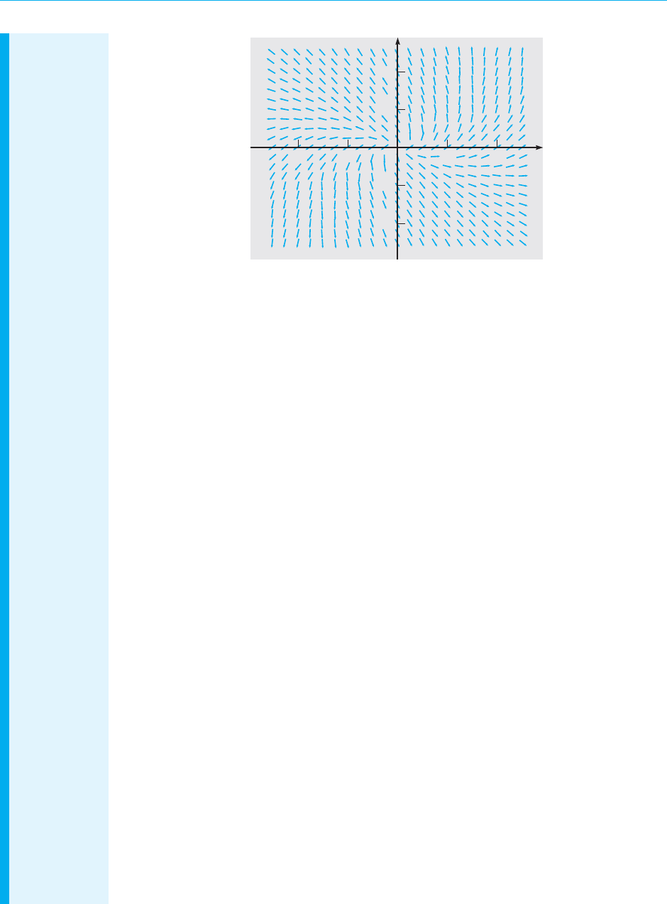
August 7, 2012 21:04 c07 Sheet number 73 Page number 431 cyan black
7.8 Repeated Eigenvalues 431
2
1
–1
–2
–2 –1 12
x
1
x
2
FIGURE 7.8.1 A direction field for the system (8).
Based on the procedure used for second order linear equations in Section 3.4, it may be
natural to attempt to find a second independent solution of the system (8) of the form
x = ξte
2t
, (10)
where ξ is a constant vector to be determined. Substituting for x in Eq. (8), we obtain
2ξte
2t
+ ξe
2t
−Aξte
2t
= 0. (11)
For Eq. (11) to be satisfied for all t, it is necessary for the coefficients of te
2t
and e
2t
both to be
zero. From the term in e
2t
we find that
ξ = 0. (12)
Hence there is no nonzero solution of the system (8) of the form (10).
Since Eq. (11) contains terms in both te
2t
and e
2t
, it appears that in addition to ξte
2t
, the
second solution must contain a term of the form ηe
2t
; in other words, we need to assume that
x = ξte
2t
+ ηe
2t
, (13)
where ξ and η are constant vectors to be determined. Upon substituting this expression for x
in Eq. (8), we obtain
2ξte
2t
+ (ξ + 2η)e
2t
= A(ξte
2t
+ ηe
2t
). (14)
Equating coefficients of te
2t
and e
2t
on each side of Eq. (14) gives the two conditions
(A − 2I)ξ = 0 (15)
and
(A − 2I)η = ξ (16)
for the determination of ξ and η. Equation (15) is satisfied if ξ is an eigenvector of A
corresponding to the eigenvalue r = 2, such as ξ
T
= (1, −1). Since det(A − 2I) is zero,
Eq. (16) is solvable only if the right side ξ satisfies a certain condition. Fortunately, ξ and

August 7, 2012 21:04 c07 Sheet number 74 Page number 432 cyan black
432 Chapter 7. Systems of First Order Linear Equations
its multiples are exactly the vectors that allow Eq. (16) to be solved. The augmented matrix for
Eq. (16) is
#
−1 −1
1
11
−1
$
.
The second row of this matrix is proportional to the first, so the system is solvable. We have
−η
1
− η
2
= 1,
so if η
1
= k, where k is arbitrary, then η
2
=−k − 1. If we write
η =
#
k
−1 − k
$
=
#
0
−1
$
+ k
#
1
−1
$
, (17)
then by substituting for ξ and η in Eq. (13), we obtain
x =
'
1
−1
(
te
2t
+
'
0
−1
(
e
2t
+ k
'
1
−1
(
e
2t
. (18)
The last term in Eq. (18) is merely a multiple of the first solution x
(1)
(t) and may be ignored,
but the first two terms constitute a new solution:
x
(2)
(t) =
#
1
−1
$
te
2t
+
#
0
−1
$
e
2t
. (19)
An elementary calculation shows that W[x
(1)
, x
(2)
](t) =−e
4t
̸= 0, and therefore x
(1)
and x
(2)
form a fundamental set of solutions of the system (8). The general solution is
x = c
1
x
(1)
(t) + c
2
x
(2)
(t)
= c
1
#
1
−1
$
e
2t
+ c
2
,#
1
−1
$
te
2t
+
#
0
−1
$
e
2t
-
. (20)
The main features of a phase portrait for the solution (20) follow from the presence of the
exponential factor e
2t
in every term.Therefore x → 0 as t →−∞and,unless both c
1
and c
2
are
zero,x becomes unbounded as t →∞.Ifc
1
and c
2
are not both zero,then along any trajectory
we have
lim
t→−∞
x
2
(t)
x
1
(t)
= lim
t→−∞
−c
1
− c
2
t − c
2
c
1
+ c
2
t
=−1.
Therefore, as t →−∞, every trajectory approaches the origin tangent to the line x
2
=−x
1
determined by the eigenvector; this behavior is clearly evident in Figure 7.8.2a. Further, as
t →∞, the slope of each trajectory also approaches −1. However, it is possible to show that
trajectories do not approach asymptotes as t →∞. Several trajectories of the system (8) are
shown in Figure 7.8.2a, and some typical plots of x
1
versus t are shown in Figure 7.8.2b.The
pattern of trajectories in this figure is typical of 2 × 2 systems x
′
= Ax with equal eigenvalues
and only one independent eigenvector. The origin is called an improper node in this case. If
the eigenvalues are negative, then the trajectories are similar but are traversed in the inward
direction. An improper node is asymptotically stable or unstable, depending on whether the
eigenvalues are negative or positive.

August 7, 2012 21:04 c07 Sheet number 75 Page number 433 cyan black
7.8 Repeated Eigenvalues 433
x
(1)
(t)
(2)
x
2
x
1
–2 –1
–1
–2
1
1
2
2
(a)
x (t)
(b)
x
1
t
1 2
2
1
–1
–2
FIGURE 7.8.2 (a) Phase portrait of the system (8); the origin is an
improper node. (b) Plots of x
1
versus t for the system (8).
One difference between a system of two first order equations and a single second
order equation is evident from the preceding example. For a second order linear
equation with a repeated root r
1
of the characteristic equation,a term ce
r
1
t
in the sec-
ond solution is not required since it is a multiple of the first solution. On the other
hand, for a system of two first order equations, the term ηe
r
1
t
of Eq. (13) with r
1
= 2
is not, in general, a multiple of the first solution ξe
r
1
t
, so the term ηe
r
1
t
must be
retained.
Example 2 is entirely typical of the general case when there is a double eigenvalue
and a single associated eigenvector. Consider again the system (1), and suppose that
r = ρ isa doubleeigenvalue ofA,but that thereis onlyone correspondingeigenvector
ξ. Then one solution [similar to Eq. (9)] is
x
(1)
(t) = ξe
ρt
, (21)
where ξ satisfies
(A − ρ I)ξ = 0. (22)
By proceeding as in Example 2, we find that a second solution [similar to Eq. (19)] is
x
(2)
(t) = ξte
ρt
+ ηe
ρt
, (23)
where ξ satisfies Eq. (22) and η is determined from
(A − ρ I)η = ξ. (24)
Even though det(A − ρI) = 0, it can be shown that it is always possible to solve
Eq. (24) for η. Note that if we multiply Eq. (24) by A − ρ I and use Eq. (22), then we
obtain
(A − ρ I)
2
η = 0.
The vector η is called a generalized eigenvector of the matrix A corresponding to the
eigenvalue ρ.
Fundamental Matrices. As explained in Section 7.7, fundamental matrices are formed
by arranging linearly independent solutions in columns. Thus, for example, a

August 7, 2012 21:04 c07 Sheet number 76 Page number 434 cyan black
434 Chapter 7. Systems of First Order Linear Equations
fundamental matrix for the system (8) can be formed from the solutions x
(1)
(t) and
x
(2)
(t) from Eqs. (9) and (19), respectively:
$(t) =
'
e
2t
te
2t
−e
2t
−te
2t
− e
2t
(
= e
2t
'
1 t
−1 −1 − t
(
. (25)
The particular fundamental matrix # that satisfies #(0) = I can also be readily found
from the relation #(t) = $(t)$
−1
(0). For Eq. (8) we have
$(0) =
'
10
−1 −1
(
, $
−1
(0) =
'
10
−1 −1
(
, (26)
and then
#(t) = $(t)$
−1
(0) = e
2t
'
1 t
−1 −1 − t
('
10
−1 −1
(
= e
2t
'
1 − t −t
t 1 + t
(
. (27)
The latter matrix is also the exponential matrix exp(At).
Jordan Forms. An n × n matrixA canbe diagonalized as discussed in Section 7.7 only if
it has a full complement of n linearly independent eigenvectors. If there is a shortage
of eigenvectors (because of repeated eigenvalues),then A can always be transformed
into a nearly diagonal matrix called its Jordan
6
form, which has the eigenvalues of
A on the main diagonal, ones in certain positions on the diagonal above the main
diagonal, and zeros elsewhere.
Consider again the matrix A given by Eq. (2). To transform A into its Jordan form,
we construct the transformation matrix T with the single eigenvector ξ from Eq. (6)
in its first column and the generalized eigenvector η from Eq. (17) with k = 0 in the
second column. Then T and its inverse are given by
T =
'
10
−1 −1
(
, T
−1
=
'
10
−1 −1
(
. (28)
As you can verify, it follows that
T
−1
AT =
'
21
02
(
= J. (29)
The matrix J in Eq. (29) is the Jordan form of A. It is typical of all Jordan forms in that
it has a 1 above the main diagonal in the column corresponding to the eigenvector
that is lacking (and is replaced in T by the generalized eigenvector).
If we start again from Eq. (1)
x
′
= Ax,
6
Marie Ennemond Camille Jordan (1838–1922) was professor at the École Polytechnique and the Collège
de France. He is known for his important contributions to analysis and to topology (the Jordan curve
theorem) and especially for his foundational work in group theory. The Jordan form of a matrix appeared
in his influential book Traité des substitutions et des équations algébriques, published in 1870.

August 7, 2012 21:04 c07 Sheet number 77 Page number 435 cyan black
7.8 Repeated Eigenvalues 435
the transformation x = Ty, where T is given by Eq. (28), produces the system
y
′
= Jy, (30)
where J is given by Eq. (29). In scalar form the system (30) is
y
′
1
= 2y
1
+ y
2
, y
′
2
= 2y
2
. (31)
These equations can be solved readily in reverse order—that is, by starting with the
equation for y
2
. In this way we obtain
y
2
= c
1
e
2t
, y
1
= c
1
te
2t
+ c
2
e
2t
. (32)
Thus two independent solutions of the system (30) are
y
(1)
(t) =
'
1
0
(
e
2t
, y
(2)
(t) =
'
t
1
(
e
2t
, (33)
and the corresponding fundamental matrix is
ˆ
$(t) =
'
e
2t
te
2t
0 e
2t
(
. (34)
Since
ˆ
$(0) = I, we can also identify the matrix in Eq. (34) as exp(Jt).The same result
can be reached by calculating powers of J and substituting them into the exponential
series (see Problems 20 through 22). To obtain a fundamental matrix for the original
system, we now form the product
$(t) = T exp(Jt) =
'
e
2t
te
2t
−e
2t
−e
2t
− te
2t
(
, (35)
which is the same as the fundamental matrix given in Eq. (25).
We will not discuss n × n systems x
′
= Ax in more detail here. For large n it is
possible that there may be eigenvalues of high algebraic multiplicity m, perhaps with
much lower geometric multiplicity q, thus giving rise to m − q generalized eigenvec-
tors. For n ≥ 4 there may also be repeated complex eigenvalues. A full discussion
7
of the Jordan form of a general n × n matrix requires a greater background in linear
algebra than we assume for most readers of this book. Problems 18 through 22 ask
you to explore the use of Jordan forms for systems of three equations.
The amount of arithmetic required in the analysis of a general n × n system may
be prohibitive to do by hand even if n is no greater than 3 or 4. Consequently,suitable
computer software should be used routinely in most cases. This does not overcome
all difficulties by any means, but it does make many problems much more tractable.
Finally, for a set of equations arising from modeling a physical system, it is likely
that some of the elements in the coefficient matrix A result from measurements of
some physical quantity. The inevitable uncertainties in such measurements lead to
uncertainties in the values of the eigenvalues of A. For example, in such a case it
may not be clear whether two eigenvalues are actually equal or are merely close
together.
7
For example, see the books listed in the References at the end of this chapter.

August 7, 2012 21:04 c07 Sheet number 78 Page number 436 cyan black
436 Chapter 7. Systems of First Order Linear Equations
PROBLEMS In each of Problems 1 through 4:
(a) Draw a direction field and sketch a few trajectories.
(b) Describe how the solutions behave as t →∞.
(c) Find the general solution of the system of equations.
1.
x
′
=
#
3 −4
1 −1
$
x 2.
x
′
=
#
4 −2
8 −4
$
x
3.
x
′
=
#
−
3
2
1
−
1
4
−
1
2
$
x 4.
x
′
=
#
−3
5
2
−
5
2
2
$
x
In each of Problems 5 and 6, find the general solution of the given system of equations.
5. x
′
=
⎛
⎜
⎝
111
21−1
0 −11
⎞
⎟
⎠
x 6. x
′
=
⎛
⎜
⎝
011
101
110
⎞
⎟
⎠
x
In each of Problems 7 through 10:
(a) Find the solution of the given initial value problem.
(b) Draw the trajectory of the solution in the x
1
x
2
-plane, and also draw the graph of x
1
versus t.
7.
x
′
=
#
1 −4
4 −7
$
x, x(0) =
'
3
2
(
8.
x
′
=
#
−
5
2
3
2
−
3
2
1
2
$
x, x(0) =
#
3
−1
$
9.
x
′
=
#
2
3
2
−
3
2
−1
$
x, x(0) =
#
3
−2
$
10.
x
′
=
#
39
−1 −3
$
x, x(0) =
#
2
4
$
In each of Problems 11 and 12:
(a) Find the solution of the given initial value problem.
(b) Draw the corresponding trajectory in x
1
x
2
x
3
-space, and also draw the graph of x
1
versus t.
11.
x
′
=
⎛
⎜
⎝
100
−410
362
⎞
⎟
⎠
x, x(0) =
⎛
⎜
⎝
−1
2
−30
⎞
⎟
⎠
12.
x
′
=
⎛
⎜
⎜
⎝
−
5
2
11
1 −
5
2
1
11−
5
2
⎞
⎟
⎟
⎠
x, x(0) =
⎛
⎜
⎝
2
3
−1
⎞
⎟
⎠
In each of Problems 13 and 14, solve the given system of equations by the method of Problem
19 of Section 7.5. Assume that t > 0.
13. tx
′
=
#
3 −4
1 −1
$
x 14. tx
′
=
#
1 −4
4 −7
$
x

August 7, 2012 21:04 c07 Sheet number 79 Page number 437 cyan black
7.8 Repeated Eigenvalues 437
15. Show that all solutions of the system
x
′
=
#
ab
cd
$
x
approach zero as t →∞if and only if a + d < 0 and ad − bc > 0. Compare this result
with that of Problem 37 in Section 3.4.
16. Consider again the electric circuit in Problem 26 of Section 7.6. This circuit is described
by the system of differential equations
d
dt
#
I
V
$
=
⎛
⎜
⎜
⎝
0
1
L
−
1
C
−
1
RC
⎞
⎟
⎟
⎠
#
I
V
$
.
(a) Show that the eigenvalues are real and equal if L = 4R
2
C.
(b) Suppose that R = 1 4, C = 1 F, and L = 4 H. Suppose also that I(0) = 1 A and
V(0) = 2 V. Find I(t) and V(t).
17. Consider again the system
x
′
= Ax =
#
1 −1
13
$
x (i)
that we discussed in Example 2.We found there that A has a double eigenvalue r
1
= r
2
= 2
with a single independent eigenvector ξ
(1)
= (1, −1)
T
, or any nonzero multiple thereof.
Thus one solution of the system (i) is x
(1)
(t) = ξ
(1)
e
2t
and a second independent solution
has the form
x
(2)
(t) = ξte
2t
+ ηe
2t
,
where ξ and η satisfy
(A − 2I)ξ = 0, (A − 2I)η = ξ. (ii)
In the text we solved the first equation for ξ and then the second equation for η. Here we
ask you to proceed in the reverse order.
(a) Show that η satisfies (A − 2I)
2
η = 0.
(b) Show that (A − 2I)
2
= 0.Thus the generalized eigenvector η can be chosen arbitrarily,
except that it must be independent of ξ
(1)
.
(c) Let η = (0, −1)
T
. Then determine ξ from the second of Eqs. (ii) and observe that
ξ = (1, −1)
T
= ξ
(1)
. This choice of η reproduces the solution found in Example 2.
(d) Let η = (1, 0)
T
and determine the corresponding eigenvector ξ.
(e) Let η = (k
1
, k
2
)
T
, where k
1
and k
2
are arbitrary numbers. Then determine ξ. How is
it related to the eigenvector ξ
(1)
?
Eigenvalues of Multiplicity 3. If the matrix A has an eigenvalue of algebraic multiplicity 3,
then there may be either one, two, or three corresponding linearly independent eigenvectors.
The general solution of the system x
′
= Ax is different, depending on the number of eigenvec-
tors associated with the triple eigenvalue. As noted in the text, there is no difficulty if there
are three eigenvectors, since then there are three independent solutions of the form x = ξe
rt
.
The following two problems illustrate the solution procedure for a triple eigenvalue with one
or two eigenvectors, respectively.

August 7, 2012 21:04 c07 Sheet number 80 Page number 438 cyan black
438 Chapter 7. Systems of First Order Linear Equations
18. Consider the system
x
′
= Ax =
⎛
⎜
⎝
111
21−1
−324
⎞
⎟
⎠
x. (i)
(a) Show that r = 2 is an eigenvalue of algebraic multiplicity 3 of the coefficient matrix
A and that there is only one corresponding eigenvector, namely,
ξ
(1)
=
⎛
⎜
⎝
0
1
−1
⎞
⎟
⎠
.
(b) Using the information in part (a), write down one solution x
(1)
(t) of the system (i).
There is no other solution of the purely exponential form x = ξe
rt
.
(c) To find a second solution, assume that x = ξte
2t
+ ηe
2t
. Show that ξ and η satisfy the
equations
(A − 2I)ξ = 0, (A − 2I)η = ξ.
Since ξ has already been found in part (a), solve the second equation for η. Neglect the
multiple of ξ
(1)
that appears in η, since it leads only to a multiple of the first solution x
(1)
.
Then write down a second solution x
(2)
(t) of the system (i).
(d) To find a third solution, assume that x = ξ(t
2
/2)e
2t
+ ηte
2t
+ ζe
2t
. Show that ξ, η, and ζ
satisfy the equations
(A − 2I)ξ = 0, (A − 2I)η = ξ, (A − 2I)ζ = η.
The first two equations are the same as in part (c), so solve the third equation for ζ, again
neglecting the multiple of ξ
(1)
that appears. Then write down a third solution x
(3)
(t) of the
system (i).
(e) Write down a fundamental matrix $(t) for the system (i).
(f) Form a matrix T with the eigenvector ξ
(1)
in the first column and the generalized
eigenvectors η and ζ in the second and third columns. Then find T
−1
and form the product
J = T
−1
AT. The matrix J is the Jordan form of A.
19. Consider the system
x
′
= Ax =
⎛
⎜
⎝
5 −3 −2
8 −5 −4
−433
⎞
⎟
⎠
x. (i)
(a) Show that r = 1 is a triple eigenvalue of the coefficient matrix A and that there are
only two linearly independent eigenvectors, which we may take as
ξ
(1)
=
⎛
⎜
⎝
1
0
2
⎞
⎟
⎠
, ξ
(2)
=
⎛
⎜
⎝
0
2
−3
⎞
⎟
⎠
. (ii)
Write down two linearly independent solutions x
(1)
(t) and x
(2)
(t) of Eq. (i).
(b) To find a third solution, assume that x = ξte
t
+ ηe
t
; then show that ξ and η must satisfy
(A − I)ξ = 0, (iii)
(A − I)η = ξ. (iv)

August 7, 2012 21:04 c07 Sheet number 81 Page number 439 cyan black
7.8 Repeated Eigenvalues 439
(c) Equation (iii) is satisfied if ξ is an eigenvector, so one way to proceed is to choose
ξ to be a suitable linear combination of ξ
(1)
and ξ
(2)
so that Eq. (iv) is solvable, and then
to solve that equation for η. However, let us proceed in a different way and follow the
pattern of Problem 17. First, show that η satisfies
(A − I)
2
η = 0.
Further, show that (A − I)
2
= 0. Thus η can be chosen arbitrarily, except that it must be
independent of ξ
(1)
and ξ
(2)
.
(d) A convenient choice for η is η = (0, 0, 1)
T
. Find the corresponding ξ from Eq. (iv).
Verify that ξ is an eigenvector.
(e) Write down a fundamental matrix $(t) for the system (i).
(f) Form a matrix T with the eigenvector ξ
(1)
in the first column and with the eigenvector
ξ from part (d) and the generalized eigenvector η in the other two columns. Find T
−1
and
form the product J = T
−1
AT. The matrix J is the Jordan form of A.
20. Let J =
#
λ 1
0 λ
$
, where λ is an arbitrary real number.
(a) Find J
2
, J
3
, and J
4
.
(b) Use an inductive argument to show that J
n
=
#
λ
n
nλ
n−1
0 λ
n
$
.
(c) Determine exp(Jt).
(d) Use exp(Jt) to solve the initial value problem x
′
= Jx, x (0) = x
0
.
21. Let
J =
⎛
⎜
⎝
λ 00
0 λ 1
00λ
⎞
⎟
⎠
,
where λ is an arbitrary real number.
(a) Find J
2
, J
3
, and J
4
.
(b) Use an inductive argument to show that
J
n
=
⎛
⎜
⎝
λ
n
00
0 λ
n
nλ
n−1
00 λ
n
⎞
⎟
⎠
.
(c) Determine exp(Jt).
(d) Observe that if you choose λ = 1, then the matrix J in this problem is the same as
the matrix J in Problem 19(f). Using the matrix T from Problem 19(f), form the product
T exp(Jt) with λ = 1. Is the resulting matrix the same as the fundamental matrix $(t) in
Problem 19(e)? If not, explain the discrepancy.
22. Let
J =
⎛
⎜
⎝
λ 10
0 λ 1
00λ
⎞
⎟
⎠
,
where λ is an arbitrary real number.
(a) Find J
2
, J
3
, and J
4
.

August 7, 2012 21:04 c07 Sheet number 82 Page number 440 cyan black
440 Chapter 7. Systems of First Order Linear Equations
(b) Use an inductive argument to show that
J
n
=
⎛
⎜
⎝
λ
n
nλ
n−1
[n(n − 1)/2]λ
n−2
0 λ
n
nλ
n−1
00 λ
n
⎞
⎟
⎠
.
(c) Determine exp(Jt).
(d) Note that if you choose λ = 2, then the matrix J in this problem is the same as the
matrix J in Problem 18(f). Using the matrix T from Problem 18(f), form the product
T exp(Jt) with λ = 2. The resulting matrix is the same as the fundamental matrix $(t) in
Problem 18(e).
7.9 Nonhomogeneous Linear Systems
In this section we turn to the nonhomogeneous system
x
′
= P(t)x + g(t), (1)
where the n × n matrix P(t) and n × 1 vector g(t) are continuous for α<t <β.By
the same argument as in Section 3.5 (see also Problem 16 in this section), the general
solution of Eq. (1) can be expressed as
x = c
1
x
(1)
(t) +···+c
n
x
(n)
(t) + v(t), (2)
where c
1
x
(1)
(t) +···+c
n
x
(n)
(t) is the general solution of the homogeneous system
x
′
= P(t)x, and v(t) is a particular solution of the nonhomogeneous system (1). We
will briefly describe several methods for determining v(t).
Diagonalization. We begin with systems of the form
x
′
= Ax + g(t), (3)
where A is an n × n diagonalizable constant matrix. By diagonalizing the coefficient
matrix A, as indicated in Section 7.7, we can transform Eq. (3) into a system of
equations that is readily solvable.
Let T be the matrix whose columns are the eigenvectors ξ
(1)
, ..., ξ
(n)
of A, and
define a new dependent variable y by
x = Ty. (4)
Then, substituting for x in Eq. (3), we obtain
Ty
′
= ATy + g(t).
When we multiply by T
−1
, it follows that
y
′
= (T
−1
AT)y +T
−1
g(t) = Dy + h(t), (5)
where h (t) = T
−1
g(t) and where D is the diagonal matrix whose diagonal entries
are the eigenvalues r
1
, ..., r
n
of A, arranged in the same order as the corresponding
eigenvectors ξ
(1)
, ..., ξ
(n)
that appear as columns of T. Equation (5) is a system of

August 7, 2012 21:04 c07 Sheet number 83 Page number 441 cyan black
7.9 Nonhomogeneous Linear Systems 441
n uncoupled equations for y
1
(t), ..., y
n
(t); as a consequence, the equations can be
solved separately. In scalar form, Eq. (5) has the form
y
′
j
(t) = r
j
y
j
(t) + h
j
(t), j = 1, ..., n, (6)
where h
j
(t) is a certain linear combination of g
1
(t), ..., g
n
(t). Equation (6) is a first
order linear equation and can be solved by the methods of Section 2.1. In fact, we
have
y
j
(t) = e
r
j
t
"
t
t
0
e
−r
j
s
h
j
(s) ds + c
j
e
r
j
t
, j = 1, ..., n, (7)
where the c
j
are arbitrary constants. Finally,the solution x of Eq. (3) is obtained from
Eq. (4). When multiplied by the transformation matrix T, the second term on the
right side of Eq. (7) produces the general solution of the homogeneous equation
x
′
= Ax, while the first term on the right side of Eq. (7) yields a particular solution of
the nonhomogeneous system (3).
EXAMPLE
1
Find the general solution of the system
x
′
=
#
−21
1 −2
$
x +
#
2e
−t
3t
$
= Ax + g(t). (8)
Proceeding as in Section 7.5, we find that the eigenvalues of the coefficient matrix are
r
1
=−3 and r
2
=−1 and that the corresponding eigenvectors are
ξ
(1)
=
#
1
−1
$
, ξ
(2)
=
#
1
1
$
. (9)
Thus the general solution of the homogeneous system is
x = c
1
#
1
−1
$
e
−3t
+ c
2
#
1
1
$
e
−t
. (10)
Before writing down the matrix T of eigenvectors, we recall that eventually we must find T
−1
.
The coefficient matrix A is real and symmetric, so we can use the result stated just above
Example 3 in Section 7.7: T
−1
is simply the adjoint or (since T is real) the transpose of T,
provided that the eigenvectors of A are normalized so that (ξ, ξ) = 1. Hence,upon normalizing
ξ
(1)
and ξ
(2)
, we have
T =
1
√
2
#
11
−11
$
, T
−1
=
1
√
2
#
1 −1
11
$
. (11)
Letting x = Ty and substituting for x in Eq. (8),we obtain the following system of equations
for the new dependent variable y:
y
′
= Dy +T
−1
g(t) =
#
−30
0 −1
$
y +
1
√
2
#
2e
−t
− 3t
2e
−t
+ 3t
$
. (12)
Thus
y
′
1
+ 3y
1
=
√
2e
−t
−
3
√
2
t,
(13)
y
′
2
+ y
2
=
√
2e
−t
+
3
√
2
t.

August 7, 2012 21:04 c07 Sheet number 84 Page number 442 cyan black
442 Chapter 7. Systems of First Order Linear Equations
Each of Eqs. (13) is a first order linear equation and so can be solved by the methods of Section
2.1. In this way we obtain
y
1
=
√
2
2
e
−t
−
3
√
2
%'
t
3
(
−
1
9
&
+ c
1
e
−3t
,
(14)
y
2
=
√
2te
−t
+
3
√
2
(t − 1) + c
2
e
−t
.
Finally, we write the solution in terms of the original variables:
x = Ty =
1
√
2
#
y
1
+ y
2
−y
1
+ y
2
$
=
⎛
⎜
⎝
(c
1
/
√
2)e
−3t
+
;
(c
2
/
√
2) +
1
2
<
e
−t
+ t −
4
3
+ te
−t
−(c
1
/
√
2)e
−3t
+
;
(c
2
/
√
2) −
1
2
<
e
−t
+ 2t −
5
3
+ te
−t
⎞
⎟
⎠
= k
1
#
1
−1
$
e
−3t
+ k
2
#
1
1
$
e
−t
+
1
2
#
1
−1
$
e
−t
+
#
1
1
$
te
−t
+
#
1
2
$
t −
1
3
#
4
5
$
, (15)
where k
1
= c
1
/
√
2 and k
2
= c
2
/
√
2. The first two terms on the right side of Eq. (15) form the
general solution of the homogeneous system corresponding to Eq. (8). The remaining terms
are a particular solution of the nonhomogeneous system.
If the coefficient matrix A in Eq. (3) is not diagonalizable (because of repeated
eigenvalues and a shortage of eigenvectors), it can nevertheless be reduced to
a Jordan form J by a suitable transformation matrix T involving both eigen-
vectors and generalized eigenvectors. In this case the differential equations for
y
1
, ..., y
n
are not totally uncoupled since some rows of J have two nonzero ele-
ments: an eigenvalue in the diagonal position anda1intheadjacent position to
the right. However, the equations for y
1
, ..., y
n
can still be solved consecutively,
starting with y
n
. Then the solution of the original system (3) can be found by the
relation x = Ty.
Undetermined Coefficients. A second way to find a particular solution of the nonho-
mogeneous system (1) is the method of undetermined coefficients that we first
discussed in Section 3.5. To use this method, we assume the form of the solution
with some or all of the coefficients unspecified, and then seek to determine these
coefficients so as to satisfy the differential equation. As a practical matter, this
method is applicable only if the coefficient matrix P is a constant matrix, and if
the components of g are polynomial, exponential, or sinusoidal functions, or sums
or products of these. In these cases the correct form of the solution can be pre-
dicted in a simple and systematic manner. The procedure for choosing the form of
the solution is substantially the same as that given in Section 3.5 for linear second
order equations. The main difference is illustrated by the case of a nonhomogeneous
term of the form ue
λt
, where λ is a simple root of the characteristic equation. In
this situation, rather than assuming a solution of the form ate
λt
, it is necessary to
use ate
λt
+ be
λt
, where a and b are determined by substituting into the differential
equation.

August 7, 2012 21:04 c07 Sheet number 85 Page number 443 cyan black
7.9 Nonhomogeneous Linear Systems 443
EXAMPLE
2
Use the method of undetermined coefficients to find a particular solution of
x
′
=
#
−21
1 −2
$
x +
#
2e
−t
3t
$
= Ax + g(t). (16)
This is the same system of equations as in Example 1. To use the method of undetermined
coefficients, we write g(t) in the form
g(t) =
#
2
0
$
e
−t
+
#
0
3
$
t. (17)
Observe that r =−1 is an eigenvalue of the coefficient matrix, and therefore we must include
both ate
−t
and be
−t
in the assumed solution. Thus we assume that
x = v(t) = ate
−t
+ be
−t
+ ct + d, (18)
where a, b, c, and d are vectors to be determined. By substituting Eq. (18) into Eq. (16) and
collecting terms, we obtain the following algebraic equations for a, b, c, and d:
Aa =−a,
Ab = a − b −
#
2
0
$
,
(19)
Ac =−
#
0
3
$
,
Ad = c.
From the first of Eqs. (19),we see that a is an eigenvector of A corresponding to the eigenvalue
r =−1. Thus a
T
= (α, α), where α is any nonzero constant. Then we find that the second of
Eqs. (19) can be solved only if α = 1 and that in this case,
b = k
#
1
1
$
−
#
0
1
$
(20)
for any constant k. The simplest choice is k = 0, from which b
T
= (0, −1). Then the third and
fourth of Eqs. (19) yield c
T
= (1, 2) and d
T
= (−
4
3
, −
5
3
), respectively. Finally, from Eq. (18) we
obtain the particular solution
v(t) =
#
1
1
$
te
−t
−
#
0
1
$
e
−t
+
#
1
2
$
t −
1
3
#
4
5
$
. (21)
The particular solution (21) is not identical to the one contained in Eq. (15) of Example 1
because the term in e
−t
is different. However,if we choose k =
1
2
in Eq. (20),then b
T
= (
1
2
, −
1
2
)
and the two particular solutions agree.
Variation of Parameters. Now let us turn to more general problems in which the
coefficient matrix is not constant or not diagonalizable. Let
x
′
= P(t)x + g(t), (22)
where P(t) and g(t) are continuous on α<t <β. Assume that a fundamental matrix
$(t) for the corresponding homogeneous system
x
′
= P(t)x (23)

August 7, 2012 21:04 c07 Sheet number 86 Page number 444 cyan black
444 Chapter 7. Systems of First Order Linear Equations
has been found. We use the method of variation of parameters to construct a partic-
ular solution, and hence the general solution, of the nonhomogeneous system (22).
Since the general solution of the homogeneous system (23) is $(t)c, it is natural to
proceed as in Section 3.6 and to seek a solution of the nonhomogeneous system (22)
by replacing the constant vector c by a vector function u(t). Thus we assume that
x = $(t)u(t), (24)
where u(t) is a vector to be found. Upon differentiating x as given by Eq. (24) and
requiring that Eq. (22) be satisfied, we obtain
$
′
(t)u(t) + $(t)u
′
(t) = P(t)$(t)u(t) + g(t). (25)
Since $(t) is a fundamental matrix, $
′
(t) = P(t)$(t); hence Eq. (25) reduces to
$(t)u
′
(t) = g(t). (26)
Recall that $(t) is nonsingular on any interval where P is continuous. Hence $
−1
(t)
exists, and therefore
u
′
(t) = $
−1
(t)g(t). (27)
Thus for u(t) we can select any vector from the class of vectors that satisfy Eq. (27).
These vectors are determined only up to an arbitrary additive constant vector;
therefore, we denote u(t) by
u(t) =
"
$
−1
(t)g(t) dt + c, (28)
where the constant vector c is arbitrary. If the integrals in Eq. (28) can be evaluated,
then the general solution of the system (22) is found by substituting for u(t) from
Eq. (28) in Eq. (24). However, even if the integrals cannot be evaluated, we can still
write the general solution of Eq. (22) in the form
x = $(t)c + $(t)
"
t
t
1
$
−1
(s)g(s) ds, (29)
where t
1
is any point in the interval (α, β).The first term on the right side of Eq. (29) is
the general solution of the corresponding homogeneous system (23), and the second
term is a particular solution of Eq. (22).
Now let us consider the initial value problem consisting of the differential equation
(22) and the initial condition
x(t
0
) = x
0
. (30)
We can find the solution of this problem most conveniently if we choose the lower
limit of integration in Eq. (29) to be the initial point t
0
. Then the general solution of
the differential equation is
x = $(t)c + $(t)
"
t
t
0
$
−1
(s)g(s) ds. (31)
For t = t
0
the integral in Eq. (31) is zero, so the initial condition (30) is also satisfied
if we choose
c = $
−1
(t
0
)x
0
. (32)

August 7, 2012 21:04 c07 Sheet number 87 Page number 445 cyan black
7.9 Nonhomogeneous Linear Systems 445
Therefore,
x = $(t)$
−1
(t
0
)x
0
+ $(t)
"
t
t
0
$
−1
(s)g(s) ds (33)
is the solution of the given initial value problem. Again, although it is helpful to use
$
−1
to write the solutions (29) and (33),it is usually better in particular cases to solve
the necessary equations by row reduction than to calculate $
−1
and substitute into
Eqs. (29) and (33).
The solution (33) takes a slightly simpler form if we use the fundamental matrix
#(t) satisfying #(t
0
) = I. In this case we have
x = #(t)x
0
+ #(t)
"
t
t
0
#
−1
(s)g(s) ds. (34)
Equation (34) can be simplified further if the coefficient matrix P(t) is a constant
matrix (see Problem 17).
EXAMPLE
3
Use the method of variation of parameters to find the general solution of the system
x
′
=
#
−21
1 −2
$
x +
#
2e
−t
3t
$
= Ax + g(t). (35)
This is the same system of equations as in Examples 1 and 2.
The general solution of the corresponding homogeneous system was given in Eq. (10). Thus
$(t) =
#
e
−3t
e
−t
−e
−3t
e
−t
$
(36)
is a fundamental matrix. Then the solution x of Eq. (35) is given by x = $(t)u(t), where u(t)
satisfies $ (t)u
′
(t) = g(t), or
#
e
−3t
e
−t
−e
−3t
e
−t
$#
u
′
1
u
′
2
$
=
#
2e
−t
3t
$
. (37)
Solving Eq. (37) by row reduction, we obtain
u
′
1
= e
2t
−
3
2
te
3t
,
u
′
2
= 1 +
3
2
te
t
.
Hence
u
1
(t) =
1
2
e
2t
−
1
2
te
3t
+
1
6
e
3t
+ c
1
,
u
2
(t) = t +
3
2
te
t
−
3
2
e
t
+ c
2
,
and
x = $(t)u(t)
= c
1
#
1
−1
$
e
−3t
+ c
2
#
1
1
$
e
−t
+
1
2
#
1
−1
$
e
−t
+
#
1
1
$
te
−t
+
#
1
2
$
t −
1
3
#
4
5
$
, (38)
which is the same as the solution obtained in Example 1 [Eq. (15)] and is equivalent to the
solution obtained in Example 2 [Eq. (21)].

August 7, 2012 21:04 c07 Sheet number 88 Page number 446 cyan black
446 Chapter 7. Systems of First Order Linear Equations
Laplace Transforms. We used the Laplace transform in Chapter 6 to solve linear equa-
tions of arbitrary order. It can also be used in very much the same way to solve
systems of equations. Since the transform is an integral, the transform of a vector is
computed component by component. Thus
L{x(t)} is the vector whose components
are the transforms of the respective components of x(t), and similarly for
L{x
′
(t)}.
We will denote
L{x(t)} by X(s). Then, by an extension of Theorem 6.2.1 to vectors,
we also have
L{x
′
(t)}=sX(s) − x(0). (39)
EXAMPLE
4
Use the method of Laplace transforms to solve the system
x
′
=
#
−21
1 −2
$
x +
#
2e
−t
3t
$
= Ax + g(t). (40)
This is the same system of equations as in Examples 1 through 3.
We take the Laplace transform of each term in Eq. (40), obtaining
sX(s) − x(0) = AX(s) + G(s), (41)
where G(s) is the transform of g(t). The transform G(s) is given by
G(s) =
#
2/(s + 1)
3/s
2
$
. (42)
To proceed further we need to choose the initial vector x(0). For simplicity let us choose
x(0) = 0. Then Eq. (41) becomes
(sI −A)X(s) = G(s), (43)
where, as usual, I is the identity matrix. Consequently, X(s) is given by
X(s) = (sI −A)
−1
G(s). (44)
The matrix (sI −A)
−1
is called the transfer matrix because multiplying it by the transform of
the input vector g(t) yields the transform of the output vector x(t). In this example we have
sI −A =
#
s + 2 −1
−1 s + 2
$
, (45)
and by a straightforward calculation, we obtain
(sI −A)
−1
=
1
(s + 1)(s + 3)
#
s + 21
1 s + 2
$
. (46)
Then, substituting from Eqs. (42) and (46) in Eq. (44) and carrying out the indicated multi-
plication, we find that
X(s) =
⎛
⎜
⎜
⎜
⎝
2(s + 2)
(s + 1)
2
(s + 3)
+
3
s
2
(s + 1)(s + 3)
2
(s + 1)
2
(s + 3)
+
3(s + 2)
s
2
(s + 1)(s + 3)
⎞
⎟
⎟
⎟
⎠
. (47)
Finally, we need to obtain the solution x(t) from its transform X(s). This can be done by
expanding the expressions in Eq. (47) in partial fractions and using Table 6.2.1, or (more

August 7, 2012 21:04 c07 Sheet number 89 Page number 447 cyan black
7.9 Nonhomogeneous Linear Systems 447
efficiently) by using appropriate computer software. In any case, after some simplification the
result is
x(t) =
#
2
1
$
e
−t
−
2
3
#
1
−1
$
e
−3t
+
#
1
1
$
te
−t
+
#
1
2
$
t −
1
3
#
4
5
$
. (48)
Equation (48) gives the particular solution of the system (40) that satisfies the initial condition
x(0) = 0. As a result, it differs slightly from the particular solutions obtained in the preceding
three examples. To obtain the general solution of Eq. (40), you must add to the expression in
Eq. (48) the general solution (10) of the homogeneous system corresponding to Eq. (40).
Each of the methods for solving nonhomogeneous equations has some advantages
and disadvantages. The method of undetermined coefficients requires no integra-
tion, but it is limited in scope and may entail the solution of several sets of algebraic
equations. The method of diagonalization requires finding the inverse of the trans-
formation matrix and the solution of a set of uncoupled first order linear equations,
followed by a matrix multiplication. Its main advantage is that for Hermitian coeffi-
cient matrices, the inverse of the transformation matrix can be written down without
calculation—a feature that is more important for large systems. The method of
Laplace transforms involves a matrix inversion to find the transfer matrix, followed
by a multiplication, and finally by the determination of the inverse transform of each
term in the resulting expression. It is particularly useful in problems with forcing
functions that involve discontinuous or impulsive terms. Variation of parameters is
the most general method. On the other hand, it involves the solution of a set of lin-
ear algebraic equations with variable coefficients, followed by an integration and a
matrix multiplication, so it may also be the most complicated from a computational
viewpoint. For many small systems with constant coefficients, such as the one in the
examples in this section,all of these methods work well,and theremay be little reason
to select one over another.
PROBLEMS In each of Problems 1 through 12 find the general solution of the given system of equations.
1. x
′
=
#
2 −1
3 −2
$
x +
#
e
t
t
$
2. x
′
=
#
1
√
3
√
3 −1
$
x +
#
e
t
√
3 e
−t
$
3. x
′
=
#
2 −5
1 −2
$
x +
#
−cos t
sin t
$
4. x
′
=
#
11
4 −2
$
x +
#
e
−2t
−2e
t
$
5. x
′
=
#
4 −2
8 −4
$
x +
#
t
−3
−t
−2
$
, t > 0
6. x
′
=
#
−42
2 −1
$
x +
#
t
−1
2t
−1
+ 4
$
, t > 0
7. x
′
=
#
11
41
$
x +
#
2
−1
$
e
t
8. x
′
=
#
2 −1
3 −2
$
x +
#
1
−1
$
e
t
9. x
′
=
#
−
5
4
3
4
3
4
−
5
4
$
x +
#
2t
e
t
$
10. x
′
=
#
−3
√
2
√
2 −2
$
x +
#
1
−1
$
e
−t

August 7, 2012 21:04 c07 Sheet number 90 Page number 448 cyan black
448 Chapter 7. Systems of First Order Linear Equations
11. x
′
=
#
2 −5
1 −2
$
x +
#
0
cos t
$
,0< t <π
12. x
′
=
#
2 −5
1 −2
$
x +
#
csc t
sec t
$
,
π
2
< t <π
13. Theelectric circuit shown in Figure7.9.1 is described by the system of differential equations
dx
dt
=
#
−
1
2
−
1
8
2 −
1
2
$
x +
#
1
2
0
$
I(t), (i)
where x
1
is the current through the inductor, x
2
is the voltage drop across the capacitor,
and I(t) is the current supplied by the external source.
(a) Determine a fundamental matrix $(t) for the homogeneous system corresponding to
Eq. (i). Refer to Problem 25 of Section 7.6.
(b) If I(t) = e
−t/2
, determine the solution of the system (i) that also satisfies the initial
conditions x(0) = 0.
I(t)
R = 4 ohms R = 4 ohms
L = 8 henrys
C = farad
1
2
FIGURE 7.9.1 The circuit in Problem 13.
In each of Problems 14 and 15, verify that the given vector is the general solution of the
corresponding homogeneous system, and then solve the nonhomogeneous system. Assume
that t > 0.
14. tx
′
=
#
2 −1
3 −2
$
x +
#
1 − t
2
2t
$
, x
(c)
= c
1
#
1
1
$
t + c
2
#
1
3
$
t
−1
15. tx
′
=
#
3 −2
2 −2
$
x +
#
−2t
t
4
− 1
$
, x
(c)
= c
1
#
1
2
$
t
−1
+ c
2
#
2
1
$
t
2
16. Let x = φ(t) be the general solution of x
′
= P(t)x + g(t), and let x = v(t) be some
particular solution of the same system. By considering the difference φ(t) − v(t), show
that φ(t) = u(t) + v(t), where u(t) is the general solution of the homogeneous system
x
′
= P(t)x.
17. Consider the initial value problem
x
′
= Ax + g(t), x(0) = x
0
.
(a) By referring to Problem 15(c) in Section 7.7, show that
x = #(t)x
0
+
"
t
0
#(t − s)g(s) ds.

August 7, 2012 21:04 c07 Sheet number 91 Page number 449 cyan black
7.9 Nonhomogeneous Linear Systems 449
(b) Show also that
x = exp(At)x
0
+
"
t
0
exp[A(t − s)]g(s) ds.
Compare these results with those of Problem 27 in Section 3.6.
18. Use the Laplace transform to solve the system
x
′
=
#
−21
1 −2
$
x +
#
2e
−t
3t
$
= Ax + g(t) (i)
used in the examples in this section. Instead of using zero initial conditions, as in Example
4, let
x(0) =
#
α
1
α
2
$
, (ii)
where α
1
and α
2
are arbitrary. How mustα
1
and α
2
be chosen so that the solution isidentical
to Eq. (38)?
REFERENCES Further information on matrices and linear algebra is available in any introductory book on the subject.
Here is a representative sample:
Anton, H. and Rorres, C., Elementary Linear Algebra (10th ed.) (Hoboken, NJ: Wiley, 2010).
Johnson, L. W., Riess, R. D., and Arnold, J. T., Introduction to Linear Algebra (6th ed.) (Boston: Addison-
Wesley, 2008).
Kolman, B. and Hill, D. R.,Elementary Linear Algebra (8th ed.) (Upper Saddle River, NJ: Pearson, 2004).
Lay, D. C., Linear Algebra and Its Applications(4th ed.)(Boston:Addison-Wesley, 2012).
Leon, S. J., Linear Algebra with Applications (8th ed.) (Upper Saddle River, NJ: Pearson/Prentice-Hall,
2010).
Strang, G., Linear Algebra and Its Applications (4th ed.)(Belmont, CA:Thomson, Brooks/Cole, 2006).
A more extended treatment of systems of first order linear equations may be found in many books,
including the following:
Coddington, E. A. and Carlson, R., Linear Ordinary Differential Equations (Philadelphia, PA: Society for
Industrial and Applied Mahematics, 1997).
Hirsch, M. W., Smale, S., and Devaney, R. L., Differential Equations, Dynamical Systems, and an Introduc-
tion to Chaos (2nd ed.)(San Diego, CA:Academic Press, 2004).
The following book treats elementary differential equations with a particular emphasis on systems of
first order equations:
Brannan, J. R. and Boyce, W. E., Differential Equations: An Introduction to Modern Methods and
Applications (2nd ed.) (New York: Wiley, 2011).
August 7, 2012 21:04 c07 Sheet number 92 Page number 450 cyan black

August 7, 2012 21:05 c08 Sheet number 1 Page number 451 cyan black
451
CHAPTER
8
Numerical
Methods
Up tothis pointwe havediscussed methods for solving differential equations by using
analytical techniques such as integration or series expansions. Usually, the emphasis
was on finding an exact expression for the solution. Unfortunately, there are many
important problems in engineering and science, especially nonlinear ones, to which
these methods either do not apply or are very complicated to use. In this chapter
we discuss an alternative approach, the use of numerical approximation methods to
obtain an accurate approximation to the solution of an initial value problem. We
present these methods in the simplest possible context, namely, a single scalar first
order equation. However, they can readily be extended to systems of first order
equations, and this is outlined briefly in Section 8.5. The procedures described here
can be executed easily on personal computers.
8.1 The Euler or Tangent Line Method
To discuss the development and use of numerical approximation procedures, we
will concentrate mainly on the first order initial value problem consisting of the
differential equation
dy
dt
= f (t, y) (1)
and the initial condition
y(t
0
) = y
0
. (2)
We assumethat the functions f and f
y
are continuous on somerectangle in the ty-plane
containing the point (t
0
, y
0
). Then, by Theorem 2.4.2, there exists a unique solution
y = φ(t) of the given problem in some interval about t
0
. If Eq. (1) is nonlinear, then

August 7, 2012 21:05 c08 Sheet number 2 Page number 452 cyan black
452 Chapter 8. Numerical Methods
the interval of existence of the solution may be difficult to determine and may have
no simple relationship to the function f . However, in all our discussions we assume
that there is a unique solution of the initial value problem (1), (2) in the interval of
interest.
In Section 2.7 we described the oldest and simplest numerical approximation
method, namely, the Euler or tangent line method. To derive this method, let us
write the differential equation (1) at the point t = t
n
in the form
d φ
dt
(t
n
) = f [t
n
, φ(t
n
)]. (3)
Then we approximate the derivative in Eq. (3) by the corresponding (forward)
difference quotient, obtaining
φ(t
n+1
) − φ(t
n
)
t
n+1
− t
n
∼
=
f [t
n
, φ(t
n
)]. (4)
Finally, if we replace φ(t
n+1
) and φ(t
n
) by their approximate values y
n+1
and y
n
,
respectively, and solve for y
n+1
, we obtain the Euler formula
y
n+1
= y
n
+ f (t
n
, y
n
)(t
n+1
− t
n
), n = 0, 1, 2, .... (5)
If the step size t
n+1
− t
n
has a uniform value h for all n and if we denote f (t
n
, y
n
) by
f
n
, then Eq. (5) simplifies to
y
n+1
= y
n
+ hf
n
, n = 0, 1, 2, .... (6)
Euler’s method consists of repeatedly evaluating Eq. (5) or (6), using the result
of each step to execute the next step. In this way we obtain a sequence of values
y
0
, y
1
, y
2
, ..., y
n
, ... that approximate the values of the solution φ(t) at the points
t
0
, t
1
, t
2
, ..., t
n
, ....
A computer program for Euler’s method has a structure such as that shown below.
The specific instructions can be written in any convenient programming language.
The Euler Method
Step 1. define f (t, y)
Step 2. input initial values t0 and y0
Step 3. input step size h and number of steps n
Step 4. output t0 and y0
Step 5. for j from 1 to n do
Step 6. k1 = f (t, y)
y = y + h ∗ k1
t = t + h
Step 7. output t and y
Step 8. end

August 7, 2012 21:05 c08 Sheet number 3 Page number 453 cyan black
8.1 The Euler or Tangent Line Method 453
Some examples of Euler’s method appear in Section 2.7. As another example,
consider the initial value problem
y
′
= 1 − t + 4y, (7)
y(0) = 1. (8)
Equation (7) is a first order linear equation,and you can easily verify that the solution
satisfying the initial condition (8) is
y = φ(t) =
1
4
t −
3
16
+
19
16
e
4t
. (9)
Since the exact solution is known, we do not need numerical methods to approx-
imate the solution of the initial value problem (7), (8). On the other hand, the
availability of the exact solution makes it easy to determine the accuracy of any
numerical procedure that we use on this problem. We will use this problem through-
out the chapter to illustrate and compare different numerical methods. The solutions
of Eq. (7) diverge rather rapidly from each other, so we should expect that it will
be fairly difficult to approximate the solution (9) well over any interval of moder-
ate length. Indeed, this is the reason for choosing this particular problem; it will be
relatively easy to observe the benefits of using more efficient methods.
EXAMPLE
1
Using the Euler formula (6) and step sizes h = 0.05, 0.025, 0.01, and 0.001, determine approx-
imate values of the solution y = φ(t) of the problem (7), (8) on the interval 0 ≤ t ≤ 2.
The indicated calculationswere carriedout on acomputer,andsome ofthe results areshown
in Table 8.1.1. Their accuracy is not particularly impressive. For h = 0.01 the percentage error
is 3.85% at t = 0.5, 7.49% at t = 1.0, and 14.4% at t = 2.0. The corresponding percentage
errors for h = 0.001 are 0.40%, 0.79%, and 1.58%, respectively. Observe that if h = 0.001,
then it requires 2000 steps to traverse the interval from t = 0tot = 2. Thus considerable
computation is needed to obtain even reasonably good accuracy for this problem using the
Euler method. When we discuss other numerical approximation methods later in this chapter,
we will find that it is possible to obtain comparable or better accuracy with much larger step
sizes and many fewer computational steps.
TABLE 8.1.1 A Comparison of Results for the Numerical Approximation of the Solution
of y
′
= 1 − t + 4y, y(0) = 1 Using the Euler Method for Different Step Sizes h
th= 0.05 h = 0.025 h = 0.01 h = 0.001 Exact
0.01.0000000 1.0000000 1.0000000 1.0000000 1.0000000
0.11.5475000 1.5761188 1.5952901 1.6076289 1.6090418
0.22.3249000 2.4080117 2.4644587 2.5011159 2.5053299
0.33.4333560 3.6143837 3.7390345 3.8207130 3.8301388
0.45.0185326 5.3690304 5.6137120 5.7754845 5.7942260
0.57.2901870 7.9264062 8.3766865 8.6770692 8.7120041
1.045.588400 53.807866 60 .037126 64.382558 64.897803
1.5 282.07187 361.75945 426.40818 473.55979 479.25919
2.0
1745
.6662 2432.7878 3029.3279 3484.1608 3540.2001

August 7, 2012 21:05 c08 Sheet number 4 Page number 454 cyan black
454 Chapter 8. Numerical Methods
To begin to investigate the errors in using numerical approximations, and also to
suggest ways to construct more accurate algorithms, it is helpful to mention some
alternative ways to look at the Euler method.
One way to proceed is to write the problem as an integral equation. Let y = φ(t)
be the solution of the initial value problem (1), (2); then, by integrating from t
n
to
t
n+1
, we obtain
"
t
n+1
t
n
φ
′
(t) dt =
"
t
n+1
t
n
f [t, φ(t)]dt,
or
φ(t
n+1
) = φ(t
n
) +
"
t
n+1
t
n
f [t, φ(t)]dt. (10)
The integral in Eq. (10) is represented geometrically as the area under the curve in
Figure 8.1.1 between t = t
n
and t = t
n+1
. If we approximate the integral by replacing
f [t, φ(t)] by its value f [t
n
, φ(t
n
)] at t = t
n
, then we are approximating the actual area
by the area of the shaded rectangle. In this way we obtain
φ(t
n+1
)
∼
=
φ(t
n
) + f [t
n
, φ(t
n
)](t
n+1
− t
n
)
= φ(t
n
) + hf [t
n
, φ(t
n
)]. (11)
Finally,to obtain an approximation y
n+1
for φ(t
n+1
),we make a second approximation
by replacing φ(t
n
) by its approximate value y
n
in Eq. (11).This gives the Euler formula
y
n+1
= y
n
+ hf (t
n
, y
n
). A more accurate algorithm can be obtained by approximating
the integral more accurately. This is discussed in Section 8.2.
y'
t
f [t
n
, (t
n
)]
φ
t
n
t
n+1
y' = f [t, (t)]
φ
FIGURE 8.1.1 Integral derivation of the Euler method.
Another approach is to assume that the solution y = φ(t) has a Taylor series about
the point t
n
. Then
φ(t
n
+ h) = φ(t
n
) + φ
′
(t
n
)h + φ
′′
(t
n
)
h
2
2!
+···,
or
φ(t
n+1
) = φ(t
n
) + f [t
n
, φ(t
n
)]h + φ
′′
(t
n
)
h
2
2!
+···. (12)
If the series is terminated after the first two terms, and φ(t
n+1
) and φ(t
n
) are replaced
by their approximate values y
n+1
and y
n
, we again obtain the Euler formula (6). If
more terms in the series are retained, a more accurate formula is obtained. Further,
by using a Taylor series with a remainder, it is possible to estimate the magnitude of
the error in the formula. This is discussed later in this section.

August 7, 2012 21:05 c08 Sheet number 5 Page number 455 cyan black
8.1 The Euler or Tangent Line Method 455
The Backward Euler Formula. A variation on the Euler formula can be obtained by
using the backward difference quotient [φ(t
n
) − φ(t
n−1
)]/h to approximate the deri-
vative in Eq. (3) instead of the forward difference quotient used in Eq. (4). In this
way we obtain
φ(t
n
) − φ(t
n−1
)
∼
=
hf (t
n
, y
n
),
or
y
n
= y
n−1
+ hf (t
n
, y
n
).
Stepping the index up from n to n + 1, we obtain the backward Euler formula
y
n+1
= y
n
+ hf (t
n+1
, y
n+1
). (13)
Assuming that y
n
is known and y
n+1
is to be calculated,observe that Eq. (13) does not
provide an explicit formula for y
n+1
. Rather, it is an equation that implicitly defines
y
n+1
and must be solved to determine the value of y
n+1
. How difficult this is depends
entirely on the nature of the function f .
EXAMPLE
2
Use the backward Euler formula (13) and step sizes h = 0.05, 0.025, 0.01, and 0.001 to find
approximate values of the solutionof theinitial value problem(7),(8) on the interval 0 ≤ t ≤ 2.
For this problem, the backward Euler formula (13) becomes
y
n+1
= y
n
+ h(1 − t
n+1
+ 4y
n+1
).
We will show the first two steps in detail so that it will be clear how the method works. At the
first step we have
y
1
= y
0
+ h(1 − t
1
+ 4y
1
) = 1 + (0.05)(1 − 0.05 + 4y
1
).
Solving this equation for y
1
, we obtain
y
1
= 1.0475/0.8 = 1.309375.
Observe that because the differential equation is linear, the implicit equation for y
1
is also
linear and therefore easy to solve. Next,
y
2
= y
1
+ h(1 − t
2
+ 4y
2
) = 1.309375 + (0.05)(1 − 0.1 + 4y
2
),
which leads to
y
2
= 1.354375/0.8 = 1.69296875.
Continuing the computations on a computer, we obtain the results shown in Table 8.1.2.
The values given by the backward Euler method are uniformly too large for this problem,
TABLE 8.1.2 A Comparison of Results for the Numerical Approximation of the Solution of
y
′
= 1 − t + 4y, y(0) = 1 Using the Backward Euler Method for Different Step Sizes h
th= 0 .05 h = 0.025 h = 0.01 h = 0.001 Exact
01.0000000 1.0000000 1.0000000 1.0000000 1.0000000
0.11.6929688 1.6474375 1.6236638 1.6104634 1.6090418
0.22.7616699 2.6211306 2.5491368 2.5095731 2.5053299
0.34.4174530 4 .0920886 3.9285724 3.8396379 3.8301388
0.46.9905516 6.3209569 5.9908303 5.8131282 5.7942260
0.510.996956 9.7050002 9.0801473 8.7472667 8.7120041
1.0 103.06171 80.402761 70.452395 65.419964 64.897803
1.5 959.44236 661.00731 542.12432 485.05825 479.25919
2.0
8934.
0696 5435.7294 4172.7228 3597.4478 3540.2001

August 7, 2012 21:05 c08 Sheet number 6 Page number 456 cyan black
456 Chapter 8. Numerical Methods
whereas the values obtained from the Euler method were too small. In this problem the errors
are somewhat larger for the backward Euler method than for the Euler method, although for
small values of h the differences are insignificant. Since the backward Euler method appears
to be no more accurate than the Euler method, and is somewhat more complicated, a natural
question is why it should even be mentioned. The answer is that it is the simplest example of a
class of methods known as backward differentiation formulas that are very useful for certain
types of differential equations. We will return to this issue later in this chapter.
Errors in Numerical Approximations. The use of a numerical procedure,such as the Euler
formula, on an initial value problem raises a number of questions that must be
answered before the approximate numerical solution can be accepted as satisfac-
tory. One of these is the question of convergence. That is, as the step size h tends
to zero, do the values of the numerical approximation y
1
, y
2
, ..., y
n
, ...approach the
corresponding values of the actual solution? If we assume that the answer is affir-
mative, there remains the important practical question of how rapidly the numerical
approximation converges to the solution. In other words, how small a step size is
needed in order to guarantee a given level of accuracy? We want to use a step size
that is small enough to ensure the required accuracy, but not too small. An unneces-
sarily small step size slows down the calculations and in some cases may even cause
a loss of accuracy.
There are three fundamental sources of error in approximating the solution of an
initial value problem numerically.
1. The formula, or algorithm, used in the calculations is an approximate one. For instance,
the Euler formula uses straight-line approximations to the actual solution.
2. Except for the first step, the input data used in the calculations are only approximations
to the actual values of the solution at the specified points.
3. The computer used for the calculations has finite precision; in other words, at each stage
only a finite number of digits can be retained.
Let us temporarily assume that our computer can execute all computations exactly;
that is, it can retain infinitely many digits (if necessary) at each step. Then the dif-
ference E
n
between the solution y = φ(t) of the initial value problem (1), (2) and its
numerical approximation y
n
at the point t = t
n
is given by
E
n
= φ(t
n
) − y
n
. (14)
The error E
n
is known as the global truncation error. It arises entirely from the
first two error sources listed above—that is, by applying an approximate formula to
approximate data.
However, in reality we must carry out the computations using finite precision
arithmetic, which means that we can keep only a finite number of digits at each step.
This leads to a round-off error R
n
defined by
R
n
= y
n
− Y
n
, (15)
where Y
n
is the value actually computed from the given numerical method.
The absolute value of the total error in computing φ(t
n
) is given by
|φ(t
n
) − Y
n
|=|φ(t
n
) − y
n
+ y
n
− Y
n
|. (16)

August 7, 2012 21:05 c08 Sheet number 7 Page number 457 cyan black
8.1 The Euler or Tangent Line Method 457
Making use of the triangle inequality, |a + b|≤|a|+|b|, we obtain, from Eq. (16),
|φ(t
n
) − Y
n
|≤|φ(t
n
) − y
n
|+|y
n
− Y
n
|
≤|E
n
|+|R
n
|. (17)
Thus the total error is bounded by the sum of the absolute values of the global
truncation and round-off errors. For the numerical procedures discussed in this book,
it is possible to obtain useful estimates of the global truncation error. The round-off
error is more difficult to analyze, since it depends on the type of computer used, the
sequence in which the computations are carried out, the method of rounding off, and
so forth. A careful examination of round-off error is beyond the scope of this book,
but see,for example,the book by Henrici listed in the references. Some of the dangers
from round-off error are discussed in Problems 25 through 27 and in Section 8.6.
It is often useful to consider separately the part of the global truncation error that
is due only to the use of an approximate formula. We can do this by assuming at the
nth step that the input data are accurate—that is, that y
n
= φ(t
n
). This error is known
as the local truncation error; we will denote it by e
n
.
Local Truncation Error for the Euler Method. Let us assume that the solution y = φ(t) of
the initial value problem (1), (2) has a continuous second derivative in the interval
of interest. To ensure this, we can assume that f , f
t
, and f
y
are continuous. For if f has
these properties and if φ is a solution of the initial value problem (1), (2), then
φ
′
(t) = f [t, φ(t)],
and, by the chain rule,
φ
′′
(t) = f
t
[t, φ(t)]+f
y
[t, φ(t)]φ
′
(t)
= f
t
[t, φ(t)]+f
y
[t, φ(t)]f [t, φ(t)]. (18)
Since the right side of this equation is continuous, φ
′′
is also continuous.
Then, making use of a Taylor polynomial with a remainder to expand φ about t
n
,
we obtain
φ(t
n
+ h) = φ(t
n
) + φ
′
(t
n
)h +
1
2
φ
′′
(t
n
)h
2
, (19)
where
t
n
is some point in t
n
< t
n
< t
n
+ h. Then, noting that φ(t
n
+ h) = φ(t
n+1
) and
φ
′
(t
n
) = f [t
n
, φ(t
n
)], we can rewrite Eq. (19) as
φ(t
n+1
) = φ(t
n
) + hf [t
n
, φ(t
n
)]+
1
2
φ
′′
(t
n
)h
2
. (20)
Now let us use the Euler formula to calculate an approximation to φ(t
n+1
) under
the assumption that we know the correct value for y
n
at t
n
, namely y
n
= φ(t
n
).The
result is
y
∗
n+1
= φ(t
n
) + hf [t
n
, φ(t
n
)], (21)
where the asterisk is used to designate this hypothetical approximate value for
φ(t
n+1
). The difference between φ(t
n+1
) and y
∗
n+1
is the local truncation error for the
(n + 1)st step in the Euler method, which we will denote by e
n+1
.Thus,by subtracting
Eq. (21) from Eq. (20), we find that
e
n+1
= φ(t
n+1
) − y
∗
n+1
=
1
2
φ
′′
(t
n
)h
2
, (22)
since the remaining terms in Eqs. (20) and (21) cancel.

August 7, 2012 21:05 c08 Sheet number 8 Page number 458 cyan black
458 Chapter 8. Numerical Methods
Thus thelocal truncation error forthe Euler method isproportional to the squareof
the step size h,and the proportionality factor depends on the second derivative of the
solution φ. The expression given by Eq. (22) depends on n and,in general, is different
for each step. A uniform bound, valid on an interval [a, b], is given by
|e
n
|≤Mh
2
/2, (23)
where M is the maximum of |φ
′′
(t)| on the interval [a, b]. Since Eq. (23) is based
on a consideration of the worst possible case—that is, the largest possible value of
|φ
′′
(t)|—it may well be a considerable overestimate of the actual local truncation
error in some parts of the interval [a, b].
One use of Eq. (23) is to choose a step size that will result in a local truncation error
no greater than some given tolerance level. For example, if the local truncation
error must be no greater than ϵ, then from Eq. (23) we have
Mh
2
/2 ≤ ϵ or h ≤
!
2ϵ/M. (24)
The primary difficulty in using Eq. (22), (23), or (24) lies in estimating |φ
′′
(t)| or M.
However, the central fact expressed by these equations is that the local truncation
error is proportional to h
2
. For example,if a new value of h is used that is one-half of
its original value, then the resulting error will be reduced to one-fourth of its previous
value.
More important than the local truncation error is the global truncation error E
n
.
The analysis for estimating E
n
is much more difficult than that for e
n
. Nevertheless,
it can be shown that the global truncation error in using the Euler method on a finite
interval is no greater than a constant times h. Thus
|E
n
|≤Kh (25)
for some constant K; see Problem 23 for more details. The Euler method is called
a first order method because its global truncation error is proportional to the first
power of the step size.
Because it is more accessible,we will hereafter use the local truncation error as our
principal measure of the accuracy of a numerical method and for comparing different
methods. If we have a priori information about the solution of the given initial value
problem,we can use the result (22) to obtain more precise information about how the
local truncation error varies with t. As an example, consider the illustrative problem
y
′
= 1 − t + 4y, y(0) = 1 (26)
on the interval 0 ≤ t ≤ 2. Let y = φ(t) be the solution of the initial value problem
(26). Then, as noted previously,
φ(t) = (4t − 3 + 19e
4t
)/16
and therefore
φ
′′
(t) = 19e
4t
.
Equation (22) then states that
e
n+1
=
19e
4t
n
h
2
2
, t
n
< t
n
< t
n
+ h. (27)

August 7, 2012 21:05 c08 Sheet number 9 Page number 459 cyan black
8.1 The Euler or Tangent Line Method 459
The appearance of the factor 19 and the rapid growth of e
4t
explain why the results
in Table 8.1.1 are not very accurate.
For instance, for h = 0.05 the error in the first step is
e
1
= φ(t
1
) − y
1
=
19e
4t
0
(0.0025)
2
,0<
t
0
< 0.05.
It is clear that e
1
is positive, and since e
4t
0
< e
0.2
, we have
e
1
≤
19e
0.2
(0.0025)
2
∼
=
0.02901. (28)
Note also that e
4t
0
> 1; hence e
1
> 19(0.0025)/2 = 0.02375. The actual error is
0.02542. It follows from Eq. (27) that the error becomes progressively worse
with increasing t; this is also clearly shown by the results in Table 8.1.1. Similar
computations for bounds for the local truncation error give
1.0617
∼
=
19e
3.8
(0.0025)
2
≤ e
20
≤
19e
4
(0.0025)
2
∼
=
1.2967 (29)
in going from 0.95 to 1.0 and
57.96
∼
=
19e
7.8
(0.0025)
2
≤ e
40
≤
19e
8
(0.0025)
2
∼
=
70.80 (30)
in going from 1.95 to 2.0.
These results indicate that for this problem, the local truncation error is about 2500
times larger near t = 2 than near t = 0. Thus, to reduce the local truncation error to
an acceptable level throughout 0 ≤ t ≤ 2, we must choose a step size h based on an
analysis near t = 2. Of course, this step size will be much smaller than necessary near
t = 0. For example, to achieve a local truncation error of 0.01 for this problem, we
need a step size of about 0.00059 near t = 2 and a step size of about 0.032 near t = 0.
The use of a uniform step size that is smaller than necessary over much of the interval
results in more calculations than necessary, more time consumed, and possibly more
danger of unacceptable round-off errors.
Another approach is to keep the local truncation error approximately constant
throughout the interval by gradually reducing the step size as t increases. In the
example problem, we would need to reduce h by a factor of about 50 in going from
t = 0tot = 2.A method that provides for variations in the step size is called adaptive.
All modern computer codes for solving differential equations have the capability of
adjusting the step size as needed. We will return to this question in the next section.

August 7, 2012 21:05 c08 Sheet number 10 Page number 460 cyan black
460 Chapter 8. Numerical Methods
PROBLEMS In each of Problems 1 through 6, find approximate values of the solution of the given initial
value problem at t = 0.1, 0.2, 0.3, and 0.4.
(a) Use the Euler method with h = 0.05.
(b) Use the Euler method with h = 0.025.
(c) Use the backward Euler method with h = 0.05.
(d) Use the backward Euler method with h = 0.025.
1.
y
′
= 3 + t − y, y(0) = 12.y
′
= 5t − 3
√
y, y(0) = 2
3.
y
′
= 2y − 3t, y(0) = 14.y
′
= 2t + e
−ty
, y(0) = 1
5.
y
′
=
y
2
+ 2ty
3 + t
2
, y(0) = 0.56. y
′
= (t
2
− y
2
) sin y, y(0) =−1
In each of Problems 7 through 12, find approximate values of the solution of the given initial
value problem at t = 0.5, 1.0, 1.5, and 2.0.
(a) Use the Euler method with h = 0.025.
(b) Use the Euler method with h = 0.0125.
(c) Use the backward Euler method with h = 0.025.
(d) Use the backward Euler method with h = 0.0125.
7.
y
′
= 0.5 − t + 2y, y(0) = 18.y
′
= 5t − 3
√
y, y(0) = 2
9.
y
′
=
√
t + y, y(0) = 3 10. y
′
= 2t + e
−ty
, y(0) = 1
11.
y
′
= (4 − ty)/(1 + y
2
), y(0) =−2
12.
y
′
= (y
2
+ 2ty)/(3 + t
2
), y(0) = 0.5
13.
Complete the calculations leading to the entries in columns three and four of Table 8.1.1.
14.
Complete the calculations leading to the entries in columns three and four of Table 8.1.2.
15. Using three terms in the Taylor series given in Eq. (12) and taking h = 0.1, determine
approximate values of the solution of the illustrative example y
′
= 1 − t + 4y, y(0) = 1at
t = 0.1 and 0.2. Compare the results with those using the Euler method and with the exact
values.
Hint: If y
′
= f (t, y), what is y
′′
?
In each of Problems 16 and 17, estimate the local truncation error for the Euler method in
terms of the solution y = φ(t). Obtain a bound for e
n+1
in terms of t and φ(t) that is valid on
the interval 0 ≤ t ≤ 1. By using a formula for the solution, obtain a more accurate error bound
for e
n+1
.Forh = 0.1 compute a bound for e
1
and compare it with the actual error at t = 0.1.
Also compute a bound for the error e
4
in the fourth step.
16. y
′
= 2y − 1, y(0) = 1 17. y
′
=
1
2
− t + 2y, y(0) = 1
In each of Problems 18 through 21,obtain a formula for the local truncation error for the Euler
method in terms of t and the solution φ.
18. y
′
= t
2
+ y
2
, y(0) = 1 19. y
′
= 5t − 3
√
y, y(0) = 2
20. y
′
=
√
t + y, y(1) = 3 21. y
′
= 2t + e
−ty
, y(0) = 1
22.
Consider the initial value problem
y
′
= cos 5πt, y(0) = 1.

August 7, 2012 21:05 c08 Sheet number 11 Page number 461 cyan black
8.1 The Euler or Tangent Line Method 461
(a) Determine the solution y = φ(t), and draw a graph of y = φ(t) for 0 ≤ t ≤ 1.
(b) Determine approximate values of φ(t) at t = 0.2, 0.4, and 0.6 using the Euler method
with h = 0.2. Draw a broken-line graph for the approximate solution,and compare it with
the graph of the exact solution.
(c) Repeat the computation of part (b) for 0 ≤ t ≤ 0.4, but take h = 0.1.
(d) Show by computing the local truncation error that neither of these step sizes is suffi-
ciently small. Determine a value of h to ensure that the local truncation error is less than
0.05 throughout the interval 0 ≤ t ≤ 1.That such a small value of h is required results from
the fact that max |φ
′′
(t)| is large.
23. In this problem we discuss the global truncation error associated with the Euler method
for the initial value problem y
′
= f (t, y), y(t
0
) = y
0
. Assuming that the functions f and f
y
are continuous in a closed,bounded region R of the ty-plane that includes the point (t
0
, y
0
),
it can be shown that there exists a constant L such that |f (t, y) − f (t,
˜
y| < L|y −
˜
y|, where
(t, y) and (t,
˜
y) are any two points in R with the same t coordinate (see Problem 15 of
Section 2.8). Further, we assume that f
t
is continuous, so the solution φ has a continuous
second derivative.
(a) Using Eq. (20), show that
|E
n+1
|≤|E
n
|+h|f [t
n
, φ(t
n
)]−f (t
n
, y
n
)|+
1
2
h
2
|φ
′′
(t
n
)|≤α|E
n
|+βh
2
, (i)
where α = 1 + hL and β = max |φ
′′
(t)|/2 on t
0
≤ t ≤ t
n
.
(b) Assume that if E
0
= 0, and if |E
n
| satisfies Eq. (i), then |E
n
|≤βh
2
(α
n
− 1)/(α − 1)
for α ̸= 1. Use this result to show that
|E
n
|≤
(1 + hL)
n
− 1
L
βh. (ii)
Equation (ii) gives a bound for |E
n
| in terms of h, L, n, and β. Notice that for a fixed h, this
error bound increases with increasing n; that is, the error bound increases with distance
from the starting point t
0
.
(c) Show that (1 + hL)
n
≤ e
nhL
; hence
|E
n
|≤
e
nhL
− 1
L
βh.
If we select an ending point T greater than t
0
and then choose the step size h so that n
steps are required to traverse the interval [t
0
, T], then nh = T − t
0
, and
|E
n
|≤
e
(T−t
0
)L
− 1
L
βh = Kh,
which is Eq. (25). Note that K depends on the length T − t
0
of the interval and on the
constants L and β that are determined from the function f .
24. Derive an expression analogous to Eq. (22) for the local truncation error for the backward
Euler formula.
Hint: Construct a suitable Taylor approximation to φ(t) about t = t
n+1
.
25.
Using a step size h = 0.05 and the Euler method,but retaining only three digits throughout
the computations, determine approximate values of the solution at t = 0.1, 0.2, 0.3, and
0.4 for each of the following initial value problems:
(a) y
′
= 1 − t + 4y, y(0) = 1
(b) y
′
= 3 + t − y, y(0) = 1
(c) y
′
= 2y − 3t, y(0) = 1

August 7, 2012 21:05 c08 Sheet number 12 Page number 462 cyan black
462 Chapter 8. Numerical Methods
Compare the results with those obtained in Example 1 and in Problems 1 and 3. The
small differences between some of those results rounded to three digits and the present
results are due to round-off error. The round-off error would become important if the
computation required many steps.
26. The following problem illustrates a danger that occurs because of round-off error when
nearly equal numbers are subtracted and the difference is then multiplied by a large
number. Evaluate the quantity
1000 ·
3
3
3
3
6.010 18.04
2.004 6.000
3
3
3
3
in the following ways:
(a) First round each entry in the determinant to two digits.
(b) First round each entry in the determinant to three digits.
(c) Retain all four digits. Compare this value with the results in parts (a) and (b).
27. The distributive law a(b − c) = ab − ac does not hold, in general, if the products are
rounded off to a smaller number of digits. To show this in a specific case, take a = 0.22,
b = 3.19, and c = 2.17. After each multiplication, round off the last digit.
8.2 Improvements on the Euler Method
Since for many problems the Euler method requires a very small step size to produce
sufficiently accurate results, much effort has been devoted to the development of
more efficient methods. In the next three sections, we will discuss some of these
methods. Consider the initial value problem
y
′
= f (t, y), y(t
0
) = y
0
(1)
and let y = φ(t) denote its solution. Recall from Eq. (10) of Section 8.1 that by
integrating the given differential equation from t
n
to t
n+1
, we obtain
φ(t
n+1
) = φ(t
n
) +
"
t
n+1
t
n
f [t, φ(t)]dt. (2)
The Euler formula
y
n+1
= y
n
+ hf (t
n
, y
n
) (3)
is obtained by replacing f [t, φ(t)] in Eq. (2) by its approximate value f (t
n
, y
n
) at the
left endpoint of the interval of integration.
Improved Euler Formula. A better approximate formula can be obtained if the
integrand in Eq. (2) is approximated more accurately. One way to do this is to
replace the integrand by the average of its values at the two endpoints, namely,
{f [t
n
, φ(t
n
)]+f [t
n+1
, φ(t
n+1
)]}/2. This is equivalent to approximating the area under
the curve in Figure 8.2.1 between t = t
n
and t = t
n+1
by the area of the shaded

August 7, 2012 21:05 c08 Sheet number 13 Page number 463 cyan black
8.2 Improvements on the Euler Method 463
trapezoid. Further, we replace φ(t
n
) and φ(t
n+1
) by their respective approximate
values y
n
and y
n+1
. In this way we obtain, from Eq. (2),
y
n+1
= y
n
+
f (t
n
, y
n
) + f (t
n+1
, y
n+1
)
2
h. (4)
Since the unknown y
n+1
appears as one of the arguments of f on the right side of
Eq. (4), this equation defines y
n+1
implicitly rather than explicitly. Depending on
the nature of the function f , it may be fairly difficult to solve Eq. (4) for y
n+1
. This
difficulty can be overcome by replacing y
n+1
on the right side of Eq. (4) by the value
obtained using the Euler formula (3). Thus
y
n+1
= y
n
+
f (t
n
, y
n
) + f [t
n
+ h, y
n
+ hf (t
n
, y
n
)]
2
h
= y
n
+
f
n
+ f (t
n
+ h, y
n
+ hf
n
)
2
h, (5)
where t
n+1
has been replaced by t
n
+ h.
y'
t
{f [t
n
, (t
n
)] +
φ
1
2
y' = f [t, (t)]
φ
f [t
n
, (t
n
)]
φ
f [t
n+1
, (t
n+1
)]}
φ
f
[t
n+1
, (t
n+1
)]
φ
t
n
t
n+1
FIGURE 8.2.1 Derivation of the improved Euler method.
Equation (5) gives an explicit formula for computing y
n+1
, the approximate value
of φ(t
n+1
), in terms of the data at t
n
. This formula is known as the improved Euler
formula or the Heun
1
formula. The improved Euler formula is an example of a two-
stage method; that is, we first calculate y
n
+ hf
n
from the Euler formula and then
use this result to calculate y
n+1
from Eq. (5). The improved Euler formula (5) is an
improvement over the Euler formula (3) because the local truncation error in using
Eq. (5) is proportional to h
3
, while for the Euler method it is proportional to h
2
. This
error estimate forthe improvedEuler formula isestablished in Problem14. It canalso
be shown that for a finite interval,the global truncation error for the improved Euler
formula is bounded by a constant times h
2
, so this method is a second order method.
Note that this greater accuracy is achieved at the expense of more computational
work, since it is now necessary to evaluate f (t, y) twice in order to go from t
n
to t
n+1
.
1
The formula is named for the German mathematician Karl Heun (1859–1929), who was a professor at
Technische Hochschule Karlsruhe.

August 7, 2012 21:05 c08 Sheet number 14 Page number 464 cyan black
464 Chapter 8. Numerical Methods
If f (t, y) depends only on t and not on y, then solving the differential equation
y
′
= f (t, y) reduces to integrating f (t). In this case the improved Euler formula (5)
becomes
y
n+1
− y
n
=
h
2
[f (t
n
) + f (t
n
+ h)], (6)
which is just the trapezoid rule for numerical integration.
EXAMPLE
1
Use the improved Euler formula (5) to calculate approximate values of the solution of the
initial value problem
y
′
= 1 − t + 4y, y(0) = 1. (7)
To make clear exactly what computations are required, we show a couple of steps in detail.
For this problem f (t, y) = 1 − t + 4y; hence
f
n
= 1 − t
n
+ 4y
n
and
f (t
n
+ h, y
n
+ hf
n
) = 1 − (t
n
+ h) + 4(y
n
+ hf
n
).
Further, t
0
= 0, y
0
= 1, and f
0
= 1 − t
0
+ 4y
0
= 5. If h = 0.025, then
f (t
0
+ h, y
0
+ hf
0
) = 1 − 0.025 + 4[1 + (0.025)(5)]=5.475.
Then, from Eq. (5),
y
1
= 1 + (0.5)(5 + 5.475)(0.025) = 1.1309375. (8)
At the second step we must calculate
f
1
= 1 − 0.025 + 4(1.1309375) = 5.49875,
y
1
+ hf
1
= 1.1309375 + (0.025)(5.49875) = 1.26840625,
and
f (t
2
, y
1
+ hf
1
) = 1 − 0.05 + 4(1.26840625) = 6.023625.
Then, from Eq. (5),
y
2
= 1.1309375 + (0.5)(5.49875 + 6.023625)(0.025) = 1.2749671875. (9)
Further results for 0 ≤ t ≤ 2 obtained by using the improved Euler method with h = 0.025
and h = 0.01 are given inTable 8.2.1.To compare the results of the improved Euler method with
those of the Euler method, note that the improved Euler method requires two evaluations of
f at each step, while the Euler method requires only one. This is significant because typically,
most of the computing time in each step is spent in evaluating f , so counting these evalua-
tions is a reasonable way to estimate the total computing effort. Thus, for a given step size h,
the improved Euler method requires twice as many evaluations of f as the Euler method.
Alternatively, the improved Euler method for step size h requires the same number of eval-
uations of f as the Euler method for step size h/2.
By referring toTable 8.2.1,you can see that the improved Euler method with h = 0.025 gives
much better results than the Euler method with h = 0.01. Note that to reach t = 2 with these
step sizes, the improved Euler method requires 160 evaluations of f , while the Euler method
requires 200. More noteworthy is that the improved Euler method with h = 0.025 is also
slightly more accurate than the Euler method with h = 0.001 (2000 evaluations of f ). In other
words, with something like one-twelfth of the computing effort, the improved Euler method
yields results for this problem that are comparable to, or a bit better than, those generated by
the Euler method. This illustrates that, compared to the Euler method, the improved Euler
method is clearly more efficient, yielding substantially better results or requiring much less
total computing effort, or both.

August 7, 2012 21:05 c08 Sheet number 15 Page number 465 cyan black
8.2 Improvements on the Euler Method 465
TABLE 8.2.1 A Comparison of Results Using the Euler and Improved Euler Methods for
the Initial Value Problem y
′
= 1 − t + 4y, y(0) = 1
Euler Improved Euler
th= 0.01 h = 0.001 h = 0.025 h = 0.01 Exact
01.0000000 1.0000000 1.0000000 1.0000000 1.0000000
0.11.5952901 1.6076289 1.6079462 1.6088585 1.6090418
0.22.4644587 2.5011159 2.5020618 2.5047827 2.5053299
0.33.7390345 3.8207130 3.8228282 3.8289146 3.8301388
0.45.6137120 5.7754845 5.7796888 5.7917911 5.7942260
0.58.3766865 8.6770692 8.6849039 8.7074637 8.7120041
1.060.037126 64.382558 64.497931 64.830722 64.897803
1.5 426.40818 473.55979 474.83402 478.51588 479.25919
2.0
3029
.3279 3484.1608 3496.6702 3532.8789 3540.2001
The percentage errors at t = 2 for the improved Euler method are 1.23% for h = 0.025 and
0.21% for h = 0.01.
A computer program for the Euler method can be readily modified to implement
the improved Euler method instead. All that is required is to replace Step 6 in the
algorithm in Section 8.1 by the following:
The Improved Euler Method
Step 6. k1 = f (t, y)
k2 = f (t + h, y + h ∗ k1)
y = y + (h/2) ∗ (k1 + k2)
t = t + h
Variation of Step Size. In Section 8.1 we mentioned the possibility of adjusting the
step size as a calculation proceeds so as to maintain the local truncation error at
a more or less constant level. The goal is to use no more steps than necessary
and, at the same time, to keep some control over the accuracy of the approxi-
mation. Here we will describe how this can be done. First we choose the error
tolerance ϵ, which is the local truncation error that we are willing to accept. Sup-
pose that after n steps we have reached the point (t
n
, y
n
). We choose a step size
h and calculate y
n+1
. Next we need to estimate the error we have made in calcu-
lating y
n+1
. Not knowing the actual solution, the best that we can do is to use a
more accurate method and repeat the calculation starting from (t
n
, y
n
). For exam-
ple, if we used the Euler method for the original calculation, we might repeat it
with the improved Euler method. Then the difference between the two calculated
values is an estimate e
est
n+1
of the error in using the original method. If the esti-
mated error is different from the error tolerance ϵ, then we adjust the step size
and repeat the calculation. The key to making this adjustment efficiently is know-
ing how the local truncation error e
n+1
depends on the step size h. For the Euler
method,thelocal truncation erroris proportional toh
2
,soto bring theestimated error
down (or up) to the tolerance level ϵ, we must multiply the original step size by the
factor
√
ϵ/e
est
n+1
.

August 7, 2012 21:05 c08 Sheet number 16 Page number 466 cyan black
466 Chapter 8. Numerical Methods
To illustrate this procedure, consider the example problem (7):
y
′
= 1 − t + 4y, y(0) = 1.
Suppose that we choose the error tolerance ϵ to be 0.05. You can verify that after one
step with h = 0.1, we obtain the values 1.5 and 1.595 from the Euler method and the
improved Euler method, respectively. Thus the estimated error in using the Euler
method is 0.095. Since this is larger than the tolerance level of 0.05, we need to adjust
the step size downward by the factor
!
0.05/0.095
∼
=
0.73. Rounding downward to
be conservative, let us choose the adjusted step size h = 0 .07. Then, from the Euler
formula, we obtain
y
1
= 1 + (0.07)f (0, 1) = 1.35
∼
=
φ(0.07).
Using the improved Euler method, we obtain y
1
= 1.39655, so the estimated error in
using the Euler formula is 0.04655, which is slightly less than the specified tolerance.
The actual error, based on a comparison with the solution itself, is somewhat greater,
namely, 0.05122.
We can follow the same procedure at each step of the calculation, thereby keeping
the local truncation error approximately constant throughout the entire numerical
process. Modern adaptive codes for solving differential equations adjust the step
size in very much this way as they proceed, although they usually use more accurate
formulas than the Euler and improved Euler formulas. Consequently, they are able
to achieve both efficiency and accuracy by using very small steps only where they
are really needed.
PROBLEMS In each of Problems 1 through 6, find approximate values of the solution of the given initial
value problem at t = 0.1, 0.2, 0.3, and 0.4. Compare the results with those obtained by the
Euler method and the backward Euler method in Section 8.1 and with the exact solution (if
available).
(a) Use the improved Euler method with h = 0 .05.
(b) Use the improved Euler method with h = 0.025.
(c) Use the improved Euler method with h = 0.0125.
1.
y
′
= 3 + t − y, y(0) = 12.y
′
= 5t − 3
√
y, y(0) = 2
3.
y
′
= 2y − 3t, y(0) = 14.y
′
= 2t + e
−ty
, y(0) = 1
5.
y
′
=
y
2
+ 2ty
3 + t
2
, y(0) = 0.56. y
′
= (t
2
− y
2
) sin y, y(0) =−1
In each of Problems 7 through 12, find approximate values of the solution of the given initial
value problem at t = 0.5, 1.0, 1.5, and 2.0.
(a) Use the improved Euler method with h = 0 .025.
(b) Use the improved Euler method with h = 0.0125.
7.
y
′
= 0.5 − t + 2y, y(0) = 18.y
′
= 5t − 3
√
y, y(0) = 2
9.
y
′
=
√
t + y, y(0) = 3 10. y
′
= 2t + e
−ty
, y(0) = 1
11.
y
′
= (4 − ty)/(1 + y
2
), y(0) =−2
12.
y
′
= (y
2
+ 2ty)/(3 + t
2
), y(0) = 0.5
13.
Complete the calculations leading to the entries in columns four and five of Table 8.2.1.

August 7, 2012 21:05 c08 Sheet number 17 Page number 467 cyan black
8.2 Improvements on the Euler Method 467
14. In this problem we establish that the local truncation error for the improved Euler for-
mula is proportional to h
3
. If we assume that the solution φ of the initial value problem
y
′
= f (t, y), y(t
0
) = y
0
has derivatives that are continuous through the third order ( f has
continuous second partial derivatives), then it follows that
φ(t
n
+ h) = φ(t
n
) + φ
′
(t
n
)h +
φ
′′
(t
n
)
2!
h
2
+
φ
′′′
(t
n
)
3!
h
3
,
where t
n
< t
n
< t
n
+ h. Assume that y
n
= φ(t
n
).
(a) Show that, for y
n+1
as given by Eq. (5),
e
n+1
= φ(t
n+1
) − y
n+1
=
φ
′′
(t
n
)h −{f [t
n
+ h, y
n
+ hf (t
n
, y
n
)]−f (t
n
, y
n
)}
2!
h +
φ
′′′
(t
n
)h
3
3!
. (i)
(b) Making use of the facts that φ
′′
(t) = f
t
[t, φ(t)]+f
y
[t, φ(t)]φ
′
(t) and that the Taylor
approximation with a remainder for a function F(t, y) of two variables is
F(a + h, b + k) = F (a, b) + F
t
(a, b)h + F
y
(a, b)k
+
1
2!
(h
2
F
tt
+ 2hkF
ty
+ k
2
F
yy
)
3
3
3
3
x=ξ,y=η
where ξ lies between a and a + h, and η lies between b and b + k, show that the first term
on the right side of Eq. (i) is proportional to h
3
plus higher order terms. This is the desired
result.
(c) Show that if f (t, y) is linear in t and y, then e
n+1
= φ
′′′
(t
n
)h
3
/6 for some t
n
with
t
n
< t
n
< t
n+1
.
Hint: What are f
tt
, f
ty
, and f
yy
?
15. Consider the improved Euler method for solving the illustrative initial value problem
y
′
= 1 − t + 4y, y(0) = 1. Using the result of Problem 14(c) and the exact solution of the
initial value problem, determine e
n+1
and a bound for the error at any step on 0 ≤ t ≤ 2.
Compare this error with the one obtained in Eq. (27) of Section 8.1 using the Euler method.
Also obtain a bound for e
1
for h = 0.05, and compare it with Eq. (28) of Section 8.1.
In each of Problems 16 and 17, use the actual solution φ(t) to determine e
n+1
and a bound
for e
n+1
at any step on 0 ≤ t ≤ 1 for the improved Euler method for the given initial value
problem. Also obtain a bound for e
1
for h = 0.1, and compare it with the similar estimate for
the Euler method and with the actual error for the improved Euler method.
16. y
′
= 2y − 1, y(0) = 1 17. y
′
= 0.5 − t + 2y, y(0) = 1
In each of Problems 18 through 21, carry out one step of the Euler method and of the
improved Euler method, using the step size h = 0.1. Suppose that a local truncation error
no greater than 0.0025 is required. Estimate the step size that is needed for the Euler method
to satisfy this requirement at the first step.
18. y
′
= 0.5 − t + 2y, y(0) = 1 19. y
′
= 5t − 3
√
y, y(0) = 2
20. y
′
=
√
t + y, y(0) = 3 21. y
′
= (y
2
+ 2ty)/(3 + t
2
), y(0) = 0.5
22. The modified Euler formula for the initial value problem y
′
= f (t, y), y(t
0
) = y
0
is given by
y
n+1
= y
n
+ hf [t
n
+
1
2
h, y
n
+
1
2
hf (t
n
, y
n
)].
Following the procedure outlined in Problem 14, show that the local truncation error in
the modified Euler formula is proportional to h
3
.

August 7, 2012 21:05 c08 Sheet number 18 Page number 468 cyan black
468 Chapter 8. Numerical Methods
In each of Problems 23 through 26,use the modified Euler formula of Problem 22 with h = 0.05
to compute approximate values of the solution of the given initial value problem at t = 0.1,
0.2, 0.3, and 0.4. Compare the results with those obtained in Problems 1 through 4.
23.
y
′
= 3 + t − y, y(0) = 1 24. y
′
= 5t − 3
√
y, y(0) = 2
25.
y
′
= 2y − 3t, y(0) = 1 26. y
′
= 2t + e
−ty
, y(0) = 1
27. Show that the modified Euler formula of Problem 22 is identical to the improved Euler
formula of Eq. (5) for y
′
= f (t, y) if f is linear in both t and y.
8.3 The Runge–Kutta Method
In preceding sections we have introduced the Euler formula, the backward Euler
formula, and the improved Euler formula as ways to approximate the solution of the
initial value problem
y
′
= f (t, y), y(t
0
) = y
0
(1)
numerically. The local truncation errors for these methods are proportional to h
2
, h
2
,
and h
3
, respectively. The Euler and improved Euler methods belong to what is now
called the Runge–Kutta
2
class of methods.
In this section we discuss the method originally developed by Runge and Kutta.
This method is now called the classic fourth order four-stage Runge–Kutta method,
but it is often referred to simply as the Runge–Kutta method, and we will follow this
practice for brevity. This method has a local truncation error that is proportional
to h
5
. Thus it is two orders of magnitude more accurate than the improved Euler
method and three orders of magnitude better than the Euler method. It is relatively
simple to use and is sufficiently accurate to handle many problems efficiently. This
is especially true of adaptive Runge–Kutta methods, in which provision is made to
vary the step size as needed. We return to this issue at the end of the section.
The Runge–Kutta formula involves a weighted average of values of f (t, y) at
different points in the interval t
n
≤ t ≤ t
n+1
. It is given by
y
n+1
= y
n
+ h
'
k
n1
+ 2k
n2
+ 2k
n3
+ k
n4
6
(
, (2)
where
k
n1
= f (t
n
, y
n
),
k
n2
= f (t
n
+
1
2
h, y
n
+
1
2
hk
n1
),
(3)
k
n3
= f (t
n
+
1
2
h, y
n
+
1
2
hk
n2
),
k
n4
= f (t
n
+ h, y
n
+ hk
n3
).
2
Carl David Runge (1856–1927), a German mathematician and physicist, worked for many years in
spectroscopy.The analysis of data led him to consider problems in numerical computation,and the Runge–
Kutta method originated in his paper on the numerical solution of differential equations in 1895. The
method was extended to systems of equations in 1901 by Martin Wilhelm Kutta (1867–1944). Kutta was
a German mathematician and aerodynamicist who is also well known for his important contributions to
classical airfoil theory.

August 7, 2012 21:05 c08 Sheet number 19 Page number 469 cyan black
8.3 The Runge–Kutta Method 469
The sum (k
n1
+ 2k
n2
+ 2k
n3
+ k
n4
)/6 can be interpreted as an average slope. Note
that k
n1
is the slope at the left end of the interval, k
n2
is the slope at the midpoint
using the Euler formula to go from t
n
to t
n
+ h/2, k
n3
is a second approximation
to the slope at the midpoint, and k
n4
is the slope at t
n
+ h using the Euler formula
and the slope k
n3
to go from t
n
to t
n
+ h.
Although in principle it is not difficult to show that Eq. (2) differs from the Taylor
expansion of the solution φ by terms that are proportional to h
5
, the algebra is
rather lengthy.
3
Thus we simply state without proof that the local truncation error
in using Eq. (2) is proportional to h
5
and that for a finite interval the global trunca-
tion error is at most a constant times h
4
. The earlier description of this method as a
fourth order four-stage method reflects the facts that the global truncation error is
of fourth order in the step size h and that there are four intermediate stages in the
calculation (the calculation of k
n1
, ..., k
n4
).
Clearly the Runge–Kutta formula, Eqs. (2) and (3), is more complicated than any
of the formulas discussed previously. This is of relatively little significance, however,
since it is not hard to write a computer program to implement this method. Such a
program has the same structure as the algorithm for the Euler method outlined in
Section 8.1. To be specific, the lines in Step 6 in the Euler algorithm must be replaced
by the following:
The Runge–Kutta Method
Step 6. k1 = f (t, y)
k2 = f (t + 0.5 ∗ h, y + 0.5 ∗ h ∗ k1)
k3 = f (t + 0.5 ∗ h, y + 0.5 ∗ h ∗ k2)
k4 = f (t + h, y + h ∗ k3)
y = y + (h/6) ∗ (k1 + 2 ∗ k2 + 2 ∗ k3 + k4)
t = t + h
Note that if f does not depend on y, then
k
n1
= f (t
n
), k
n2
= k
n3
= f (t
n
+ h/2), k
n4
= f (t
n
+ h), (4)
and Eq. (2) reduces to
y
n+1
− y
n
=
h
6
[f (t
n
) + 4f (t
n
+ h/2) + f (t
n
+ h)]. (5)
Equation (5) can be identified as Simpson’s
4
rule for the approximate evaluation of
the integral of y
′
= f (t). The fact that Simpson’s rule has an error proportional to h
5
is consistent with the local truncation error in the Runge–Kutta formula.
3
See, for example, Chapter 3 of the book by Henrici listed in the references.
4
Simpson’s rule is named for Thomas Simpson (1710–1761), an English mathematician and textbook
author, who published it in 1743.

August 7, 2012 21:05 c08 Sheet number 20 Page number 470 cyan black
470 Chapter 8. Numerical Methods
EXAMPLE
1
Use the Runge–Kutta method to calculate approximate values of the solution y = φ(t) of the
initial value problem
y
′
= 1 − t + 4y, y(0) = 1. (6)
Taking h = 0.2, we have
k
01
= f (0, 1) = 5; hk
01
= 1.0,
k
02
= f (0 + 0.1, 1 + 0.5) = 6.9; hk
02
= 1.38,
k
03
= f (0 + 0.1, 1 + 0.69) = 7.66; hk
03
= 1.532,
k
04
= f (0 + 0.2, 1 + 1.532) = 10.928.
Thus
y
1
= 1 +
0.2
6
[5 + 2(6.9) + 2(7.66) + 10.928]
= 1 + 1.5016 = 2.5016.
Further results using the Runge–Kutta method with h = 0.2,h = 0.1,and h = 0.05 are given
in Table 8.3.1. Note that the Runge–Kutta method yields a value at t = 2 that differs from the
exact solution by only 0.122% if the step size is h = 0.1, and by only 0.00903% if h = 0.05.
In the latter case, the error is less than one part in 10,000, and the calculated value at t = 2is
correct to four digits.
For comparison, note that both the Runge–Kutta method with h = 0.05 and the improved
Euler method with h = 0.025 require 160 evaluations of f to reach t = 2. The improved Euler
method yields a result at t = 2 that is in error by 1.23%. Although this error may be acceptable
for some purposes, it is more than 135 times the error yielded by the Runge–Kutta method
with comparable computing effort. Note also that the Runge–Kutta method with h = 0.2,
o
r
40 evaluations of f , produces a value at t = 2 with an error of 1.40%, which is only slightly
greater than the error in the improved Euler method with h = 0.025, or 160 evaluations of f .
Thus we see again that a more accurate algorithm is more efficient; it produces better results
with similar effort, or similar results with less effort.
TABLE 8.3.1 A Comparison of Results for the Numerical Approximation of the Solution
of the Initial Value Problem y
′
= 1 − t + 4y, y(0) = 1
Improved
Euler Runge–Kutta Exact
th= 0.025 h = 0.2 h = 0.1 h = 0.05
01.0000000 1.0000000 1.0000000 1.0000000 1.0000000
0.11.6079462 1.6089333 1.6090338 1.6090418
0.22.5020618 2.5016000 2.5050062 2.5053060 2.5053299
0.33.8228282 3.8294145 3.8300854 3.8301388
0.45.7796888 5.7776358 5.7927853 5.7941197 5.7942260
0.58.6849039 8.7093175 8.7118060 8.7120041
1.064.497931 64.441579 64.858107 64.894875 64.897803
1.5 474.83402 478.81928 479.22674 479.25919
2.0 3496.6702 3490.5574 3535.8667
3539
.8804 3540.2001
The classic Runge–Kutta methodsuffers fromthe sameshortcoming as other meth-
ods with a fixed step size for problems in which the local truncation error varies
widely over the interval of interest. That is, a step size that is small enough to achieve

August 7, 2012 21:05 c08 Sheet number 21 Page number 471 cyan black
8.3 The Runge–Kutta Method 471
satisfactory accuracy in some parts of the interval may be much smaller than neces-
sary in other parts of the interval. This has stimulated the development of adaptive
Runge–Kutta methods that provide for modifying the step size automatically as the
computation proceeds, so as to maintain the local truncation error near or below a
specified tolerance level. As explained in Section 8.2, this requires the estimation of
the local truncation error at each step. One way to do this is to repeat the compu-
tation with a fifth order method—which has a local truncation error proportional
to h
6
—and then to use the difference between the two results as an estimate of the
error. If this is done in a straightforward manner, then the use of the fifth order
method requires at least five more evaluations of f at each step, in addition to those
required originally by the fourth order method. However,if we make an appropriate
choice of the intermediate points and the weighting coefficients in the expressions for
k
n1
, ..., k
n4
in a certain fourth order Runge–Kutta method, then these expressions
can be used again, together with one additional stage, in a corresponding fifth order
method. This results in a substantial gain in efficiency. It turns out that this can be
done in more than one way.
The first fourth and fifth order Runge–Kutta pair was developed by Erwin
Fehlberg
5
in the late 1960s and is now called the Runge–Kutta–Fehlberg, or RKF,
6
method. The popularity of the RKF method was considerably enhanced by the
appearance in 1977 of its Fortran implementation RKF45 by Lawrence F. Shampine
and H.A.Watts.The RKF methodand other adaptive Runge–Kutta methods are very
powerful and efficient means of approximating numerically the solutions of an enor-
mous class of initial value problems. Specific implementations of one or more of them
are widely available in commercial software packages.
PROBLEMS In each of Problems 1 through 6, find approximate values of the solution of the given initial
value problem at t = 0.1, 0.2, 0.3, and 0.4. Compare the results with those obtained by using
other methods and with the exact solution (if available).
(a) Use the Runge-Kutta method with h = 0.1.
(b) Use the Runge-Kutta method with h = 0.05.
1.
y
′
= 3 + t − y, y(0) = 12. y
′
= 5t − 3
√
y, y(0) = 2
3.
y
′
= 2y − 3t, y(0) = 14.y
′
= 2t + e
−ty
, y(0) = 1
5.
y
′
=
y
2
+ 2ty
3 + t
2
, y(0) = 0.56. y
′
= (t
2
− y
2
) sin y, y(0) =−1
In each of Problems 7 through 12, find approximate values of the solution of the given initial
value problem at t = 0.5, 1.0, 1.5, and 2.0. Compare the results with those obtained by other
methods.
(a) Use the Runge–Kutta method with h = 0.1.
(b) Use the Runge–Kutta method with h = 0.05.
5
Erwin Fehlberg (1911–1990) was born in Germany, received his doctorate from the Technical University
of Berlin in 1942, emigrated to the United States after World War II, and was employed by NASA for
many years. The Runge–Kutta–Fehlberg method was first published in a NASATechnical Report in 1969.
6
The details of the RKF method may be found, for example, in the books by Ascher and Petzold and by
Mattheij and Molenaar that are listed in the references.

August 7, 2012 21:05 c08 Sheet number 22 Page number 472 cyan black
472 Chapter 8. Numerical Methods
7. y
′
= 0.5 − t + 2y, y(0) = 18.y
′
= 5t − 3
√
y, y(0) = 2
9.
y
′
=
√
t + y, y(0) = 3 10. y
′
= 2t + e
−ty
, y(0) = 1
11.
y
′
= (4 − ty)/(1 + y
2
), y(0) =−2
12.
y
′
= (y
2
+ 2ty)/(3 + t
2
), y(0) = 0.5
13.
Confirm the results in Table 8.3.1 by executing the indicated computations.
14.
Consider the initial value problem
y
′
= t
2
+ y
2
, y(0) = 1.
(a) Draw a direction field for this equation.
(b) Use the Runge–Kutta method or another method to find approximate values of the
solution at t = 0.8, 0.9, and 0.95. Choose a small enough step size so that you believe your
results are accurate to at least four digits.
(c) Try to extend the calculations in part (b) to obtain an accurate approximation to the
solution at t = 1. If you encounter difficulties in doing this, explain why you think this
happens. The direction field in part (a) may be helpful.
15.
Consider the initial value problem
y
′
= 3t
2
/(3y
2
− 4), y(0) = 0.
(a) Draw a direction field for this equation.
(b) Estimate how far the solution can be extended to theright. Let t
M
be the right endpoint
of the interval of existence of this solution. What happens at t
M
to prevent the solution
from continuing farther?
(c) Use the Runge–Kutta method with various step sizes to determine an approximate
value of t
M
.
(d) If you continue the computation beyond t
M
, you can continue to generate values of y.
What significance, if any, do these values have?
(e) Suppose that the initial condition is changed to y(0) = 1. Repeat parts (b) and (c) for
this problem.
8.4 Multistep Methods
In previous sections we have discussed numerical procedures for approximating the
solution of the initial value problem
y
′
= f (t, y), y(t
0
) = y
0
, (1)
in which data at the point t = t
n
are used to calculate an approximate value of the
solution φ(t
n+1
) at the next mesh point t = t
n+1
. In other words, the calculated value
of φ at any mesh point depends only on the data at the preceding mesh point. Such
methods are called one-step methods. However, once approximate values of the
solution y = φ(t) have been obtained at a few points beyond t
0
, it is natural to ask
whether we can make use of some of this information, rather than just the value at
the last point, to calculate the value of φ(t) at the next point. Specifically, if y
1
at t
1
,
y
2
at t
2
, ..., y
n
at t
n
are known, how can we use this information to determine y
n+1
at

August 7, 2012 21:05 c08 Sheet number 23 Page number 473 cyan black
8.4 Multistep Methods 473
t
n+1
? Methods that use information at more than the last mesh point are referred to
as multistep methods. In this section we will describe two types of multistep methods:
Adams
7
methods and backward differentiation methods. Within each type, we can
achieve various levels of accuracy,depending on the number of preceding data points
that are used. For simplicity, we will assume throughout our discussion that the step
size h is constant.
Adams Methods. Recall that
φ(t
n+1
) − φ(t
n
) =
"
t
n+1
t
n
φ
′
(t) dt, (2)
where φ(t) is the solution of the initial value problem (1).The basic idea of an Adams
method is to approximate φ
′
(t) by a polynomial P
k
(t) of degree k and to use the
polynomial to evaluate the integral on the right side of Eq. (2). The coefficients in
P
k
(t) are determined by using k + 1 previously calculated data points. For example,
suppose that we wish to use a first degree polynomial P
1
(t) = At + B. Then we need
only the two data points (t
n
, y
n
) and (t
n−1
, y
n−1
).ForP
1
to be an approximation to
φ
′
, we require that P
1
(t
n
) = f (t
n
, y
n
) and that P
1
(t
n−1
) = f (t
n−1
, y
n−1
). Recall that we
denote f (t
j
, y
j
) by f
j
for an integer j. Then A and B must satisfy the equations
At
n
+ B = f
n
,
(3)
At
n−1
+ B = f
n−1
.
Solving for A and B, we obtain
A =
f
n
− f
n−1
h
, B =
f
n−1
t
n
− f
n
t
n−1
h
. (4)
Replacing φ
′
(t) by P
1
(t) and evaluating the integral in Eq. (2), we find that
φ(t
n+1
) − φ(t
n
) =
A
2
(t
2
n+1
− t
2
n
) + B(t
n+1
− t
n
).
Finally, we replace φ(t
n+1
) and φ(t
n
) by y
n+1
and y
n
, respectively, and carry out some
algebraic simplification. For a constant step size h, we obtain
y
n+1
= y
n
+
3
2
hf
n
−
1
2
hf
n−1
. (5)
Equation (5) is the second orderAdams–Bashforth
8
formula. It is an explicit formula
for y
n+1
in terms of y
n
and y
n−1
and has a local truncation error proportional to h
3
.
We note in passing that the first order Adams–Bashforth formula, based on the
polynomial P
0
(t) = f
n
of degree zero, is just the original Euler formula.
7
John Couch Adams (1819–1892),an English mathematician and astronomer, is most famous as codiscov-
erer, with Joseph Leverrier, of the planet Neptune in 1846. He was associated with Cambridge University
for most of his life, as student (1839–1843), fellow, Lowdean Professor, and director of the Observa-
tory. Adams was extremely skilled at computation; his procedure for numerical integration of differential
equations appeared in 1883 in a book with Francis Bashforth on capillary action.
8
Francis Bashforth (1819–1912), English mathematician and Anglican priest, was a classmate of J. C.
Adams at Cambridge. He was particularly interested in ballistics and invented the Bashforth chronograph
for measuring the velocity of artillery projectiles.

August 7, 2012 21:05 c08 Sheet number 24 Page number 474 cyan black
474 Chapter 8. Numerical Methods
More accurate Adams formulas can be obtained by following the procedure out-
lined above, but using a higher degree polynomial and correspondingly more data
points. For example, suppose that a polynomial P
3
(t) of degree three is used. The
coefficients are determined from the four points (t
n
, y
n
), (t
n−1
, y
n−1
), (t
n−2
, y
n−2
), and
(t
n−3
, y
n−3
). Substituting this polynomial for φ
′
(t) in Eq. (2), evaluating the integral,
and simplifying the result, we eventually obtain the fourth order Adams–Bashforth
formula
y
n+1
= y
n
+ (h/24)(55f
n
− 59f
n−1
+ 37f
n−2
− 9f
n−3
). (6)
The local truncation error of this fourth order formula is proportional to h
5
.
A variation on the derivation of the Adams–Bashforth formulas gives another set
of formulas called the Adams–Moulton
9
formulas. To see the difference, let us again
considerthesecondorder case.Again we use afirst degree polynomial Q
1
(t) = αt + β,
but we determine the coefficients by using the points (t
n
, y
n
) and (t
n+1
, y
n+1
). Thus α
and β must satisfy
αt
n
+ β = f
n
,
(7)
αt
n+1
+ β = f
n+1
,
and it follows that
α =
f
n+1
− f
n
h
, β =
f
n
t
n+1
− f
n+1
t
n
h
. (8)
Substituting Q
1
(t) for φ
′
(t) in Eq. (2) and simplifying, we obtain
y
n+1
= y
n
+
1
2
hf
n
+
1
2
hf (t
n+1
, y
n+1
), (9)
which is the second order Adams–Moulton formula. We have written f (t
n+1
, y
n+1
)
in the last term to emphasize that the Adams–Moulton formula is implicit, rather
than explicit, since the unknown y
n+1
appears on both sides of the equation. The
local truncation error for the second order Adams–Moulton formula is proportional
to h
3
.
The first order Adams–Moulton formula is just the backward Euler formula, as
you might anticipate by analogy with the first order Adams–Bashforth formula.
More accurate higher order formulas can be obtained by using an approximating
polynomial of higher degree. The fourth orderAdams–Moulton formula,with a local
truncation error proportional to h
5
, is
y
n+1
= y
n
+ (h/24)(9f
n+1
+ 19f
n
− 5f
n−1
+ f
n−2
). (10)
Observe that this is also an implicit formula, because y
n+1
appears in f
n+1
.
Although both the Adams–Bashforth and Adams–Moulton formulas of the same
order have local truncation errors proportional to the same power of h, the Adams–
Moulton formulas of moderate order are in fact considerably more accurate.
For example, for the fourth order formulas (6) and (10), the proportionality constant
9
Forest Ray Moulton (1872–1952), an American astronomer and administrator of science, was for many
years professor of astronomy at the University of Chicago. During World War I, he was in charge of
the Ballistics Branch of the U.S. Army at Aberdeen (MD) Proving Ground. In the course of calculating
ballistics trajectories he devised substantial improvements in the Adams formula.

August 7, 2012 21:05 c08 Sheet number 25 Page number 475 cyan black
8.4 Multistep Methods 475
for the Adams–Moulton formula is less than 1/10 of the proportionality constant
for the Adams–Bashforth formula. Thus the question arises: is it better to use the
explicit (and faster) Adams–Bashforth formula or the more accurate but implicit
(and slower) Adams–Moulton formula? The answer depends on whether, by using
the more accurate formula, you can increase the step size, and thereby reduce the
number of steps enough to compensate for the additional computations required at
each step.
In fact, numerical analysts have attempted to achieve both simplicity and accuracy
by combining the two formulas in what is called a predictor–corrector method. Once
y
n−3
, y
n−2
, y
n−1
, and y
n
are known, we can compute f
n−3
, f
n−2
, f
n−1
, and f
n
, and then
use the Adams–Bashforth (predictor) formula (6) to obtain a first value for y
n+1
.
Then we compute f
n+1
and use the Adams–Moulton (corrector) formula (10), which
is no longer implicit,to obtain an improved value of y
n+1
. We can, of course,continue
to use the corrector formula (10) if the change in y
n+1
is too large. However, if it is
necessary to use the corrector formula more than once or perhaps twice, it means
that the step size h is too large and should be reduced.
In order to use any of the multistep methods, it is necessary first to calculate a few
y
j
by some other method. For example, the fourth order Adams–Moulton method
requires values for y
1
and y
2
, while the fourth order Adams–Bashforth method also
requires avalue for y
3
. Oneway to proceed is to use aone-step method of comparable
accuracy to calculate the necessary starting values. Thus, for a fourth order multistep
method,we might use the fourth order Runge–Kutta method to calculate the starting
values. This is the method used in the next example.
Another approach is to use a low order method with a very small h to calculate y
1
,
and then to increase gradually both the order and the step size until enough starting
values have been determined.
EXAMPLE
1
Consider again the initial value problem
y
′
= 1 − t + 4y, y(0) = 1. (11)
With a step size of h = 0.1, determine an approximate value of the solution y = φ(t) at t = 0.4
using the fourth order Adams–Bashforth formula, the fourth order Adams–Moulton formula,
and the predictor–corrector method.
For starting data, we use the values of y
1
, y
2
, and y
3
found by the Runge–Kutta method.
These are tabulated in Table 8.3.1. Next, calculating the corresponding values of f (t, y),we
obtain
y
0
= 1, f
0
= 5,
y
1
= 1.6089333, f
1
= 7.3357332,
y
2
= 2.5050062, f
2
= 10.820025,
y
3
= 3.8294145, f
3
= 16.017658.
Then, from the Adams–Bashforth formula, Eq. (6), we find that y
4
= 5.7836305. The exact
value of the solution at t = 0.4, correct through eight digits, is 5.7942260, so the error is
−0.0105955.
The Adams–Moulton formula, Eq. (10), leads to the equation
y
4
= 4.9251275 + 0.15y
4
,
from which it follows that y
4
= 5.7942676 with an error of only 0 .0000416.

August 7, 2012 21:05 c08 Sheet number 26 Page number 476 cyan black
476 Chapter 8. Numerical Methods
Finally, using the result from the Adams–Bashforth formula as a predicted value of φ(0.4),
we can then use Eq. (10) as a corrector. Corresponding to the predicted value of y
4
, we find
that f
4
= 23.734522. Hence, from Eq. (10), the corrected value of y
4
is 5.7926721. This result is
in error by −0.0015539.
Observe that the Adams–Bashforth method is the simplest and fastest of these methods,
since it involves only the evaluation of a single explicit formula. It is also the least accurate.
Using the Adams–Moulton formula as a corrector increases the amount of calculation that
is required, but the method is still explicit. In this problem the error in the corrected value
of y
4
is reduced by approximately a factor of 7 when compared to the error in the predicted
value. The Adams–Moulton method alone yields by far the best result, with an error that is
about 1/40 as large as the error from the predictor–corrector method. Remember, however,
that the Adams–Moulton method is implicit, which means that an equation must be solved
at each step. In the problem considered here this equation is linear, so the solution is quickly
found, but in other problems this part of the procedure may be much more time-consuming.
The Runge–Kutta method with h = 0.1 gives y
4
= 5.7927853 with an error of −0.0014407;
see Table 8.3.1. Thus, for this problem, the Runge–Kutta method is comparable in accuracy to
the predictor–corrector method.
Backward Differentiation Formulas. Another type of multistep methoduses a polynomial
P
k
(t) to approximate the solution φ(t) of the initial value problem (1) rather than
its derivative φ
′
(t), as in the Adams methods. We then differentiate P
k
(t) and set
P
′
k
(t
n+1
) equal to f (t
n+1
, y
n+1
) to obtain an implicit formula for y
n+1
. These are called
backward differentiation formulas. These methods became widely used in the 1970s
because of the work of C. William Gear
10
on so-called stiff differential equations,
whose solutions are very difficult to approximate by the methods discussed up to
now; see Section 8.6.
The simplest case uses a first degree polynomial P
1
(t) = At + B. The coefficients
are chosen to match the computed values of the solution y
n
and y
n+1
. Thus A and B
must satisfy
At
n
+ B = y
n
,
(12)
At
n+1
+ B = y
n+1
.
Since P
′
1
(t) = A, the requirement that
P
′
1
(t
n+1
) = f (t
n+1
, y
n+1
)
is just
A = f (t
n+1
, y
n+1
). (13)
Another expression for A comes from subtracting the first of Eqs. (12) from the
second, which gives
A = (y
n+1
− y
n
)/h.
10
C.William Gear (1935– ), born in London,England, received his undergraduate education at Cambridge
University and his doctorate in 1960 from the University of Illinois. He was a member of the faculty at the
University of Illinois for most of his career and made significant contributions to both computer design
and numerical analysis. His influential book on numerical methods for differential equations is listed in
the references.

August 7, 2012 21:05 c08 Sheet number 27 Page number 477 cyan black
8.4 Multistep Methods 477
Substituting this value of A into Eq. (13) and rearranging terms, we obtain the first
order backward differentiation formula
y
n+1
= y
n
+ hf (t
n+1
, y
n+1
). (14)
Note that Eq. (14) is just the backward Euler formula that we first saw in Section 8.1.
By using higher order polynomials and correspondingly more data points, we can
obtain backward differentiation formulas of any order. The second order formula is
y
n+1
=
1
3
[
4y
n
− y
n−1
+ 2hf (t
n+1
, y
n+1
)
]
, (15)
and the fourth order formula is
y
n+1
=
1
25
[
48y
n
− 36y
n−1
+ 16y
n−2
− 3y
n−3
+ 12hf (t
n+1
, y
n+1
)
]
. (16)
These formulas have local truncation errors proportional to h
3
and h
5
, respectively.
EXAMPLE
2
Use the fourth order backward differentiation formula with h = 0.1 and the data given in
Example 1 to determine an approximate value of the solution y = φ(t) at t = 0.4 for the initial
value problem (11).
Using Eq. (16) with n = 3, h = 0.1, and with y
0
, ..., y
3
given in Example 1, we obtain the
equation
y
4
= 4.6837842 + 0.192y
4
.
Thus
y
4
= 5.7967626.
Comparing the calculated value with the exact value φ(0.4) = 5.7942260, we find that the error
is 0.0025366. This is somewhat better than the result using the Adams–Bashforth method, but
it is not as good as the result using the predictor–corrector method, and not nearly as good as
the result using the Adams–Moulton method.
A comparison between one-step and multistep methods must take several factors
into consideration. The fourth order Runge–Kutta method requires four evaluations
of f at each step, while the fourth order Adams–Bashforth method (once past the
starting values) requires only one, and the predictor–corrector method only two.
Thus, for a given step size h, the latter two methods may well be considerably faster
than Runge–Kutta. However,if Runge–Kutta is more accurate and therefore can use
fewer steps, then the difference in speed will be reduced and perhaps eliminated.The
Adams–Moulton and backward differentiation formulas also require that the diffi-
culty in solving the implicit equation at each step be taken into account. All multistep
methods have the possible disadvantage that errors in earlier steps can feed back into
later calculations with unfavorable consequences. On the other hand, the underly-
ing polynomial approximations in multistep methods make it easy to approximate
the solution at points between the mesh points, should this be desirable. Multistep
methods have become popular largely because it is relatively easy to estimate the
error at each step and to adjust the order or the step size to control it. For a further
discussion of such questions as these, see the books listed at the end of this chapter;
in particular, Shampine (1994) is an authoritative source.

August 7, 2012 21:05 c08 Sheet number 28 Page number 478 cyan black
478 Chapter 8. Numerical Methods
PROBLEMS In each of Problems 1 through 6, determine an approximate value of the solution at t = 0.4
and t = 0.5 using the specified method. For starting values,use the values given by the Runge–
Kutta method; see Problems 1 through 6 of Section 8.3. Compare the results of the various
methods with each other and with the actual solution (if available).
(a) Use the fourth order predictor–corrector method with h = 0.1. Use the corrector formula
once at each step.
(b) Use the fourth order Adams–Moulton method with h = 0.1.
(c) Use the fourth order backward differentiation method with h = 0.1.
1.
y
′
= 3 + t − y, y(0) = 12.y
′
= 5t − 3
√
y, y(0) = 2
3.
y
′
= 2y − 3t, y(0) = 14.y
′
= 2t + e
−ty
, y(0) = 1
5.
y
′
=
y
2
+ 2ty
3 + t
2
, y(0) = 0.56. y
′
= (t
2
− y
2
) sin y, y(0) =−1
In each of Problems 7 through 12, find approximate values of the solution of the given initial
value problem at t = 0.5, 1.0, 1.5, and 2.0, using the specified method. For starting values,
use the values given by the Runge–Kutta method; see Problems 7 through 12 in Section 8.3.
Compare the results of the various methods with each other and with the actual solution (if
available).
(a) Use the fourth orderpredictor–corrector method with h = 0.05. Use the correctorformula
once at each step.
(b) Use the fourth order Adams–Moulton method with h = 0.05.
(c) Use the fourth order backward differentiation method with h = 0.05.
7.
y
′
= 0.5 − t + 2y, y(0) = 18.y
′
= 5t − 3
√
y, y(0) = 2
9.
y
′
=
√
t + y, y(0) = 3 10. y
′
= 2t + e
−ty
, y(0) = 1
11.
y
′
= (4 − ty)/(1 + y
2
), y(0) =−2
12.
y
′
= (y
2
+ 2ty)/(3 + t
2
), y(0) = 0.5
13. Show that the first order Adams–Bashforth method is the Euler method and that the first
order Adams–Moulton method is the backward Euler method.
14. Show that the third order Adams–Bashforth formula is
y
n+1
= y
n
+ (h/12)(23f
n
− 16f
n−1
+ 5f
n−2
).
15. Show that the third order Adams–Moulton formula is
y
n+1
= y
n
+ (h/12)(5f
n+1
+ 8f
n
− f
n−1
).
16. Derive the second order backwarddifferentiation formula givenby Eq. (15)in this section.
8.5 Systems of First Order Equations
In the preceding sections we discussed numerical methods for approximating the
solution of an initial value problem associated with a first order differential equation.
These methods can also be applied to a system of first order equations. Since a
higher order equation can always be reduced to a system of first order equations,

August 7, 2012 21:05 c08 Sheet number 29 Page number 479 cyan black
8.5 Systems of First Order Equations 479
it is sufficient to deal with systems of first order equations alone. For simplicity, we
consider a system of two first order equations
x
′
= f (t, x, y), y
′
= g(t, x, y), (1)
with the initial conditions
x(t
0
) = x
0
, y(t
0
) = y
0
. (2)
The functions f and g are assumed to satisfy the conditions of Theorem 7.1.1 so that
the initial value problem (1), (2) has a unique solution in some interval of the t-axis
containing the point t
0
. We wish to determine approximate values x
1
, x
2
, ..., x
n
, ...
and y
1
, y
2
, ..., y
n
, ...of the solution x = φ(t), y = ψ(t) at the points t
n
= t
0
+ nh with
n = 1, 2,....
In vector notation, the initial value problem (1), (2) can be written as
x
′
= f(t, x), x(t
0
) = x
0
, (3)
where x is the vector with components x and y, f is the vector function with com-
ponents f and g, and x
0
is the vector with components x
0
and y
0
. The methods of
the previous sections can be readily generalized to handle systems of two (or more)
equations. All that is needed (formally) is to replace the scalar variable x by the vec-
tor x and the scalar function f by the vector function f in the appropriate equations.
For example, the Euler formula becomes
x
n+1
= x
n
+ hf
n
, (4)
or, in component form,
'
x
n+1
y
n+1
(
=
'
x
n
y
n
(
+ h
'
f (t
n
, x
n
, y
n
)
g(t
n
, x
n
, y
n
)
(
. (5)
The initialconditions are used todetermine f
0
,whichis thevector tangent to thegraph
of the solution x = φ(t) at the initial point x
0
in the xy-plane. We move in the direc-
tion of this tangent vector for a time step h in order to find the next point x
1
. Then
we calculate a new tangent vector f
1
at x
1
, move along it for a time step h to find x
2
,
and so forth.
In a similar way, the Runge–Kutta method can be extended to a system. For the
step from t
n
to t
n+1
we have
x
n+1
= x
n
+ (h/6)(k
n1
+ 2k
n2
+ 2k
n3
+ k
n4
), (6)
where
k
n1
= f(t
n
, x
n
),
k
n2
= f[t
n
+ (h/2), x
n
+ (h/2)k
n1
],
(7)
k
n3
= f[t
n
+ (h/2), x
n
+ (h/2)k
n2
],
k
n4
= f(t
n
+ h, x
n
+ hk
n3
).
The formulas for the Adams–Moulton predictor–corrector method as it applies to
the initial value problem (1), (2) are given in Problem 9.
The vector equations (3), (4), (6), and (7) are, in fact, valid in any number of
dimensions. All that is needed is to interpret the vectors as having n components
rather than two.

August 7, 2012 21:05 c08 Sheet number 30 Page number 480 cyan black
480 Chapter 8. Numerical Methods
EXAMPLE
1
Determine approximate values of the solution x = φ(t), y = ψ(t) of the initial value problem
x
′
= x − 4y, y
′
=−x + y, (8)
x(0) = 1, y(0) = 0, (9)
at the point t = 0.2. Use the Euler method with h = 0.1 and the Runge–Kutta method with
h = 0.2. Compare the results with the values of the exact solution:
φ(t) =
e
−t
+ e
3t
2
, ψ(t) =
e
−t
− e
3t
4
. (10)
Let us first use the Euler method. For this problem, f
n
= x
n
− 4y
n
and g
n
=−x
n
+ y
n
; hence
f
0
= 1 − (4)(0) = 1, g
0
=−1 + 0 =−1.
Then, from the Euler formulas (4) and (5), we obtain
x
1
= 1 + (0.1)(1) = 1.1, y
1
= 0 + (0.1)(−1) =−0.1.
At the next step,
f
1
= 1.1 − (4)(−0.1) = 1.5, g
1
=−1.1 + (−0.1) =−1.2.
Consequently,
x
2
= 1.1 + (0.1)(1.5) = 1.25, y
2
=−0.1 + (0.1)(−1.2) =−0.22.
The values of the exact solution, correct to eight digits, are φ(0.2) = 1.3204248 and
ψ(0.2) =−0.25084701. Thus the values calculated from the Euler method are in error by
about 0.0704 and 0.0308, respectively, corresponding to percentage errors of about 5.3% and
12.3%.
Now let us use the Runge–Kutta method to approximate φ(0.2) and ψ(0.2). With h = 0.2
we obtain the following values from Eqs. (7):
k
01
=
#
f (1, 0)
g(1, 0)
$
=
#
1
−1
$
;
k
02
=
#
f (1.1, −0.1)
g(1.1, −0.1)
$
=
#
1.5
−1.2
$
;
k
03
=
#
f (1.15, −0.12)
g(1.15, −0.12)
$
=
#
1.63
−1.27
$
;
k
04
=
#
f (1.326, −0.254)
g(1.326, −0.254)
$
=
#
2.342
−1.580
$
.
Then, substituting these values in Eq. (6), we obtain
x
1
=
'
1
0
(
+
0.2
6
'
9.602
−7.52
(
=
'
1.3200667
−0.25066667
(
.
These values of x
1
and y
1
are in error by about 0.000358 and 0.000180, respectively, with
percentage errors much less than one-tenth of 1%.
This example again illustrates the great gains in accuracy that are obtainable by using a more
accurate approximation method,such as the Runge–Kuttamethod. In the calculations we have
just outlined, the Runge–Kutta method requires only twice as many function evaluations as
the Euler method, but the error in the Runge–Kutta method is about 200 times less than that
in the Euler method.

August 7, 2012 21:05 c08 Sheet number 31 Page number 481 cyan black
8.5 Systems of First Order Equations 481
PROBLEMS In each of Problems 1 through 6, determine approximate values of the solution x = φ(t),
y = ψ(t) of the given initial value problem at t = 0.2, 0.4, 0.6, 0.8, and 1.0. Compare the results
obtained by different methods and different step sizes.
(a) Use the Euler method with h = 0.1.
(b) Use the Runge–Kutta method with h = 0.2.
(c) Use the Runge–Kutta method with h = 0.1.
1.
x
′
= x + y + t, y
′
= 4x − 2y; x(0) = 1, y(0) = 0
2.
x
′
= 2x + ty, y
′
= xy; x(0) = 1, y(0) = 1
3.
x
′
=−tx − y − 1, y
′
= x; x(0) = 1, y(0) = 1
4.
x
′
= x − y + xy, y
′
= 3x − 2y − xy; x(0) = 0, y(0) = 1
5.
x
′
= x(1 − 0.5x − 0.5y), y
′
= y(−0.25 + 0.5x); x(0) = 4, y(0) = 1
6.
x
′
= exp(−x + y) − cos x, y
′
= sin(x − 3y); x(0) = 1, y(0) = 2
7.
Consider the example problem x
′
= x − 4y, y
′
=−x + y with the initial conditions
x(0) = 1 and y(0) = 0. Use the Runge–Kutta method to find approximate values of
the solution of this problem on the interval 0 ≤ t ≤ 1. Start with h = 0.2, and then
repeat the calculation with step sizes h = 0.1, 0.05, ..., each half as long as in the preceding
case. Continue the process until the first five digits of the solution at t = 1 are unchanged
for successive step sizes. Determine whether these digits are accurate by comparing them
with the exact solution given in Eqs. (10) in the text.
8.
Consider the initial value problem
x
′′
+ t
2
x
′
+ 3x = t, x(0) = 1, x
′
(0) = 2.
Convert this problem to a system of two first order equations, and determine approximate
values of the solution at t = 0.5 and t = 1.0 using the Runge–Kutta method with h = 0.1.
9.
Consider the initial value problem x
′
= f (t, x, y) and y
′
= g(t, x, y) with x(t
0
) = x
0
and
y(t
0
) = y
0
. The generalization of the Adams–Moulton predictor–corrector method of
Section 8.4 is
x
n+1
= x
n
+
1
24
h(55f
n
− 59f
n−1
+ 37f
n−2
− 9f
n−3
),
y
n+1
= y
n
+
1
24
h(55g
n
− 59g
n−1
+ 37g
n−2
− 9g
n−3
)
and
x
n+1
= x
n
+
1
24
h(9f
n+1
+ 19f
n
− 5f
n−1
+ f
n−2
),
y
n+1
= y
n
+
1
24
h(9g
n+1
+ 19g
n
− 5g
n−1
+ g
n−2
).
Determine an approximate value of the solution at t = 0.4 for the example initial value
problem x
′
= x − 4y, y
′
=−x + y with x(0) = 1, y(0) = 0. Take h = 0.1. Correct the pre-
dicted value once. For the values of x
1
, ..., y
3
use the values of the exact solution rounded
to six digits:x
1
= 1.12735, x
2
= 1.32042, x
3
= 1.60021, y
1
=−0.111255, y
2
=−0.250847,
and y
3
=−0.429696.

August 7, 2012 21:05 c08 Sheet number 32 Page number 482 cyan black
482 Chapter 8. Numerical Methods
8.6 More on Errors; Stability
In Section 8.1 we discussed some ideas related to the errors that can occur in a
numerical approximation of the solution of the initial value problem
y
′
= f (t, y), y(t
0
) = y
0
. (1)
In this section we continue that discussion and also point out some other difficulties
that can arise. Some of the points that we wish to make are fairly difficult to treat in
detail, so we will illustrate them by means of examples.
Truncation an d Round-off Errors. Recall that for the Euler method we showed that the
localtruncationerror is proportional to h
2
andthatfor a finite interval,theglobal trun-
cation error is at most a constant times h. In general,for a method of order p,the local
truncation error is proportional to h
p+1
and the global truncation error on a finite
interval is bounded by a constant times h
p
.To achieve high accuracy,we normally use
a numerical procedure for which p is fairly large, perhaps 4 or higher. As p increases,
the formula used in computing y
n+1
normally becomes more complicated, and hence
more calculations are required at each step. However, this is usually not a serious
problem unless f (t, y) is very complicated or the calculation must be repeated very
many times. If the step size h is decreased, the global truncation error is decreased by
the same factor raised to the power p. However,as we mentioned in Section 8.1,if h is
very small,a great many steps will be required to cover a fixed interval,and the global
round-off error may be larger than the global truncation error.The situation is shown
schematically in Figure 8.6.1. We assume that the round-off error R
n
is proportional
to the number of computations performed and therefore is inversely proportional to
the step size h. On the other hand,the truncation error E
n
is proportional to a positive
power of h. From Eq. (17) of Section 8.1, we know that the total error is bounded by
|E
n
|+|R
n
|; hence we wish to choose h so as to minimize this quantity. The optimum
value of h occurs when the rate of increase of the truncation error (as h increases) is
balanced by the rate of decrease of the round-off error, as indicated in Figure 8.6.1.
Error
⏐E
n
⏐ + ⏐R
n
⏐
⏐R
n
⏐
⏐E
n
⏐
hh
opt
FIGURE 8.6.1 The dependence of truncation and round-off errors on the step size h.
EXAMPLE
1
Consider the example problem
y
′
= 1 − t + 4y, y(0) = 1. (2)
Using the Euler method with various step sizes, calculate approximate values for the solution
φ(t) at t = 0.5 and t = 1. Try to determine the optimum step size.

August 7, 2012 21:05 c08 Sheet number 33 Page number 483 cyan black
8.6 More on Errors; Stability 483
Keeping only four digits in order to shorten the calculations, we obtain the data shown in
Table 8.6.1. The first two columns are the step size h and the number of steps N required to
traverse the interval 0 ≤ t ≤ 1. Then y
N/2
and y
N
are approximations to φ(0.5) = 8.712 and
φ(1) = 64 .90, respectively. These quantities appear in the third and fifth columns. The fourth
and sixth columns display the differences between the calculated values and the actual value
of the solution.
TABLE 8.6.1 Approximations to the Solution of the Initial Value
Problem y
′
= 1 − t + 4y, y(0) = 1 Using the Euler Method with
Different Step Sizes
hNy
N/2
Error y
N
Error
0.01 100 8.390 0.322 60.12 4.78
0.005 200 8.551 0.161 62.51 2.39
0.002 500 8.633 0.079 63.75 1.15
0.001 1000 8.656 0.056 63.94 0.96
0.0008 1250 8.636 0.076 63.78 1.12
0.000625 1600 8.616 0.096 64.35 0.55
0.0005 2000 8.772 0.060 64 .00 0.90
0.0004 2500 8.507 0.205 63.40 1.50
0.00025 4000 8.231 0.481 56.77 8.13
For relatively large step sizes, the round-off error is much less than the global truncation
error. Consequently, the total error is approximately the same as the global truncation error,
which for the Euler method is bounded by a constant times h. Thus, as the step size is reduced,
the error is reduced proportionally.Thefirst three lines inTable 8.6.1 show this type of behavior.
For h = 0.001 the error has been further reduced, but much less than proportionally; this
indicates that round-off error is becoming important. As h is reduced still more, the error
begins to fluctuate, and further improvements in accuracy become problematical. For values
of h less than 0.0005, the error is clearly increasing, which indicates that round-off error is
now the dominant part of the total error.
These results can also be expressed in terms of the number of steps N.ForN less than
about 1000, accuracy is improved by taking more steps, while for N greater than about 2000,
using more steps has an adverse effect. Thus for this problem it is best to use an N somewhere
between 1000 and 2000. For the calculations shown in Table 8.6.1, the best result at t = 0.5
occurs for N = 1000, while at t = 1.0 the best result is for N = 1600.
You should be careful not to read too much into the results shown in Example 1.
The optimum ranges for h and N depend on the differential equation, the numerical
method that is used, and the number of digits that are retained in the calculation.
Nevertheless, it is generally true that if too many steps are required in a calculation,
then eventually round-off error is likely to accumulate to the point where it seriously
degrades the accuracy of the procedure. For many problems this is not a concern:
for them, any of the fourth order methods we have discussed in Sections 8.3 and 8.4
will produce good results with a number of steps far less than the level at which
round-off error becomes important. For some problems, however, round-off error
does become vitally important. For such problems, the choice of method may be
crucial. This is also one reason why modern codes provide a means of adjusting
the step size as they go along, using a larger step size wherever possible and a very
small step size only where necessary.

August 7, 2012 21:05 c08 Sheet number 34 Page number 484 cyan black
484 Chapter 8. Numerical Methods
Vertical Asymptotes. As a second example, consider the problem of approximating the
solution y = φ(t) of
y
′
= t
2
+ y
2
, y(0) = 1. (3)
Since the differential equation is nonlinear,the existence and uniqueness theorem
(Theorem 2.4.2) guarantees only that there is a solution in some interval about t = 0.
Suppose that we try to compute an approximation to the solution of the initial value
problem on the interval 0 ≤ t ≤ 1 using different numerical procedures.
If we use the Euler method with h = 0.1, 0.05, and 0.01, we find the follow-
ing approximate values at t = 1: 7.189548, 12.32093, and 90.75551, respectively. The
large differences among the computed values are convincing evidence that we should
use a more accurate numerical procedure—the Runge–Kutta method, for exam-
ple. Using the Runge–Kutta method with h = 0.1, we find the approximate value
735.0991at t = 1,whichis quite differentfrom those obtainedusing the Euler method.
Repeating the calculations using step sizes of h = 0.05 and h = 0.01, we obtain the
information shown in Table 8.6.2.
TABLE 8.6.2 Approximations to the Solution
of the Initial Value Problem y
′
= t
2
+ y
2
,
y(0) = 1 Using the Runge–Kutta Method
ht= 0.90 t = 1.0
0.114.02182 735.0991
0.05 14.27117 1.75863 × 10
5
0.01 14.30478 2.0913 × 10
2893
0.001 14.30486
The values at t = 0.90 are reasonable, and we might well believe that the solution
has a value of about 14.305 at t = 0.90. However, it is not clear what is happen-
ing between t = 0.9 and t = 1.0. To help clarify this, let us turn to some analytical
approximations to thesolution of theinitial value problem(3). Note thaton 0 ≤ t ≤ 1,
y
2
≤ t
2
+ y
2
≤ 1 + y
2
. (4)
This suggests that the solution y = φ
1
(t) of
y
′
= 1 + y
2
, y(0) = 1 (5)
and the solution y = φ
2
(t) of
y
′
= y
2
, y(0) = 1 (6)
are upper and lower bounds, respectively, for the solution y = φ(t) of the original
problem,since all these solutions pass through the same initial point. Indeed,it can be
shown (for example, by the iteration method of Section 2.8) that φ
2
(t) ≤ φ(t) ≤ φ
1
(t)

August 7, 2012 21:05 c08 Sheet number 35 Page number 485 cyan black
8.6 More on Errors; Stability 485
as long as these functions exist. The important thing to note is that we can solve
Eqs. (5) and (6) for φ
1
and φ
2
by separation of variables. We find that
φ
1
(t) = tan
)
t +
π
4
*
, φ
2
(t) =
1
1 − t
. (7)
Thus φ
2
(t) →∞as t → 1, and φ
1
(t) →∞as t → π/4
∼
=
0.785. These calculations
show that the solution of the original initial value problem exists at least for
0 ≤ t <π/4 and at most for 0 ≤ t < 1. The solution of the problem (3) has a vertical
asymptote for some t in π/4 ≤ t ≤ 1 and thus does not exist on the entire interval
0 ≤ t ≤ 1.
Our numerical calculations, however, suggest that we can go beyond t = π/4, and
probably beyond t = 0.9. Assuming that the solution of the initial value problem
exists at t = 0.9 and has the value 14.305, we can obtain a more accurate estimate of
what happens for larger t by considering the initial value problems (5) and (6) with
y(0) = 1 replaced by y(0.9) = 14.305. Then we obtain
φ
1
(t) = tan(t + 0.60100), φ
2
(t) = 1/(0.96991 − t), (8)
where five decimal places have been kept in the calculation.Therefore, φ
1
(t) →∞as
t → π/2 − 0.60100
∼
=
0.96980 and φ
2
(t) →∞as t → 0.96991. We conclude that the
asymptote of the solution of the initial value problem (3) lies between these two
values. This example illustrates the sort of information that can be obtained by a
judicious combination of analytical and numerical work.
Stability. The concept of stability is associated with the possibility that small errors
that are introduced in the course of a mathematical procedure may die out as the
procedure continues. Conversely, instability occurs if small errors tend to increase,
perhaps without bound. For example, in Section 2.5 we identified equilibrium solu-
tions of a differential equation as (asymptotically) stable or unstable, depending on
whether solutions that were initiallynear theequilibrium solution tendedto approach
it or to depart from it as t increased. Somewhat more generally, the solution of an
initial value problem is asymptotically stable if initially nearby solutions tend to
approach the given solution, and unstable if they tend to depart from it. Visually, in
an asymptotically stable problem the graphs of solutions will come together, while
in an unstable problem they will separate.
If we are investigating an initial value problem numerically, the best that we can
hope for is that the numerical approximation will mimic the behavior of the actual
solution. We cannot make an unstable problem into a stable one merely by approx-
imating its solution numerically. However, it may well happen that a numerical
procedure will introduce instabilities that were not part of the original problem, and
this can cause trouble in approximating the solution. Avoidance of such instabilities
may require us to place restrictions on the step size h.
To illustrate what can happen in the simplest possible context, consider the
differential equation
dy/dt = ry, (9)
where r is a constant. Suppose that in approximating the solution of this equation,
we have reached the point (t
n
, y
n
). Let us compare the exact solution of Eq. (9) that

August 7, 2012 21:05 c08 Sheet number 36 Page number 486 cyan black
486 Chapter 8. Numerical Methods
passes through this point, namely,
y = y
n
exp[r(t − t
n
)], (10)
with numerical approximations obtained from the Euler formula
y
n+1
= y
n
+ hf (t
n
, y
n
) (11)
and from the backward Euler formula
y
n+1
= y
n
+ hf (t
n+1
, y
n+1
). (12)
From the Euler formula (11) we obtain
y
n+1
= y
n
+ hry
n
= y
n
(1 + rh). (13)
Similarly, from the backward Euler formula (12) we have
y
n+1
= y
n
+ hry
n+1
,
or
y
n+1
=
y
n
1 − rh
= y
n
[1 + rh + (rh)
2
+···]. (14)
Finally, evaluating the solution (10) at t
n
+ h, we find that
y
n+1
= y
n
exp(rh) = y
n
%
1 + rh +
(rh)
2
2
+···
&
. (15)
Comparing Eqs. (13), (14), and (15), we see that the errors in both the Euler formula
and the backward Euler formula are of order h
2
, as the theory predicts.
Now suppose that we change the value y
n
to y
n
+ δ. Think, if you wish, of δ as the
error that has accumulated by the time we reach t = t
n
. The question is whether this
error increases or decreases in going one more step to t
n+1
.
For the exact solution (15), the change in y
n+1
due to the change δ in y
n
is just
δ exp(rh). This quantity is less than δ if exp(rh)<1, or in other words if r < 0. This
confirms our conclusion in Chapter 2 that Eq. (9) is asymptotically stable if r < 0,
and is unstable if r > 0.
For thebackward Euler method,the change iny
n+1
in Eq. (14) due toδ isδ/(1 − rh).
For r < 0 the quantity 1/(1 − rh) is always nonnegative and less than 1. Thus, if the
differential equation is stable, then so is the backward Euler method for an arbitrary
step size h.
On the other hand, for the Euler method, the change in y
n+1
in Eq. (13) due to
δ is δ(1 + rh).Forr < 0 we can write 1 + rh as 1 −|r|h. Then the requirement that
|1 + rh| < 1 is equivalent to
−1 < 1 −|r|h < 1, or 0 < |r|h < 2.
Consequently, h must satisfy h < 2/|r|. Thus the Euler method is not stable for this
problem unless h is sufficiently small.
The restriction on the step size h in using the Euler method in the preceding
example is rather mild unless |r| is quite large. Nonetheless, the example illustrates
that it may be necessary to restrict h in order to achieve stability in the numerical
method, even though the initial value problem itself is stable for all values of h.
Problems for which a much smaller step size is needed for stability than for accuracy

August 7, 2012 21:05 c08 Sheet number 37 Page number 487 cyan black
8.6 More on Errors; Stability 487
are called stiff. The backward differentiation formulas described in Section 8.4 (of
which the backward Euler formula is the lowest order example) are the most popular
formulas for dealing with stiff problems.The following example illustrates the kind of
instability that can occur when we try to approximate the solution of a stiff problem.
EXAMPLE
2
AStiff
Problem
Consider the initial value problem
y
′
=−100y + 100t + 1, y(0) = 1. (16)
Find numerical approximations to the solution for 0 ≤ t ≤ 1 using the Euler, backward Euler,
and Runge–Kutta methods. Compare the numerical results with the exact solution.
Since the differential equation is linear, it is easy to solve, and the solution of the initial
value problem (16) is
y = φ(t) = e
−100t
+ t. (17)
Some values of the solution φ(t),correct to sixdecimal places,are given in the second column of
Table 8.6.3,and a graph of the solution is shown in Figure 8.6.2.There is a thin layer (sometimes
called a boundary layer) to the right of t = 0 in which the exponential term is significant
and the solution varies rapidly. Once past this layer, however, φ(t)
∼
=
t and the graph of the
solution is essentially a straight line. The width of the boundary layer is somewhat arbitrary,
but it is certainly small. At t = 0.1, for example, exp(−100t)
∼
=
0.000045.
TABLE 8.6.3 Numerical Approximations to the Solution of the Initial Value Problem
y
′
=−100y + 100t + 1, y(0) = 1
t Exact Euler Euler Runge–Kutta Runge–Kutta Backward Euler
0.025 0.0166 ... 0.0333 ... 0.025 0.1
0.01.000000 1.000000 1.000000 1.000000 1.000000 1.000000
0.05 0.056738 2.300000 −0.246296 0.470471
0.10.100045 5.162500 0.187792 10.6527 0.276796 0.190909
0.20.200000 25.8289 0.207707 111.559 0.231257 0.208264
0.40.400000 657.241 0.400059 1.24 × 10
4
0.400977 0.400068
0.60.600000 1.68 × 10
4
0.600000 1.38 × 10
6
0.600031 0.600001
0.80.800000 4.31 × 10
5
0.800000 1.54 × 10
8
0.800001 0.800000
1.01.000000 1.11 × 10
7
1.000000 1.71 × 10
10
1.000000 1.000000
1
0.8
0.6
0.4
0.2
t
0.8 10.60.40.2
y
FIGURE 8.6.2 The solution of the initial value problem y
′
=−100y + 100t + 1, y(0) = 1.

August 7, 2012 21:05 c08 Sheet number 38 Page number 488 cyan black
488 Chapter 8. Numerical Methods
If we plan to approximate the solution (17) numerically, we might intuitively expect that a
small step size will be needed only in the boundary layer. To make this expectation a bit more
precise, recall from Section 8.1 that the local truncation errors for the Euler and backward
Euler methods are proportional to φ
′′
(t). For this problem φ
′′
(t) = 10
4
e
−100t
, which varies from
a value of 10
4
at t = 0 to nearly zero for t > 0.2. Thus a very small step size is needed for
accuracy near t = 0, but a much larger step size is adequate once t is a little larger.
On the other hand, the stability analysis in Eqs. (9) through (15) also applies to this problem.
Since r =−100 for Eq. (16), it follows that for stability we need h < 0.02 for the Euler method,
but there is no corresponding restriction for the backward Euler method.
Some results obtained from the Euler method are shown in columns three and four of
Table 8.6.3. The values for h = 0.025 are worthless because of instability, while those for
h = 0.01666 ... are reasonably accurate for t ≥ 0.2. However, comparable accuracy for this
range of t is obtained for h = 0.1 by using the backward Euler method, as shown by the results
in column seven of the table.
The situation is not improved by using, instead of the Euler method, a more accurate one,
such as Runge–Kutta. For this problem the Runge–Kutta method is unstable for h = 0.033 ...
but stable for h = 0.025, as shown by the results in columns five and six of Table 8.6.3.
The results given in the table for t = 0.05 and for t = 0.1 show that in the boundary layer,
a smaller step size is needed to obtain an accurate approximation. You are invited to explore
this matter further in Problem 3.
The following example illustrates some other difficulties that may be encountered
in dealing with numerical approximations for unstable differential equations.
EXAMPLE
3
Consider the task of finding numerical approximations to two linearly independent solutions
of the second order linear equation
y
′′
− 10π
2
y = 0 (18)
for t > 0. Note any difficulties that may arise.
Since we contemplate a numerical approach to this problem, we first convert Eq. (18) into
a system of two first order equations so that we can use the methods of Section 8.5. Thus we
let x
1
= y and x
2
= y
′
. In this way we obtain the system
x
′
1
= x
2
, x
′
2
= 10π
2
x
1
,
or, if x = (x
1
, x
2
)
T
,
x
′
=
#
01
10π
2
0
$
x. (19)
The eigenvalues and eigenvectors of the coefficient matrix in Eq. (19) are
r
1
=
√
10π, ξ
(1)
=
#
1
√
10π
$
; r
2
=−
√
10π, ξ
(2)
=
#
1
−
√
10π
$
, (20)
so two linearly independent solutions of the system (19) are
x
(1)
(t) =
#
1
√
10π
$
e
√
10πt
, x
(2)
(t) =
#
1
−
√
10π
$
e
−
√
10πt
. (21)

August 7, 2012 21:05 c08 Sheet number 39 Page number 489 cyan black
8.6 More on Errors; Stability 489
The corresponding solutions of the second order equation (18) are the first components of
x
(1)
(t) and x
(2)
(t): y
1
(t) = e
√
10πt
and y
2
(t) = e
−
√
10πt
, respectively.
We also wish to consider another pair of linearly independent solutions obtained by forming
linear combinations of x
(1)
(t) and x
(2)
(t):
x
(3)
(t) =
1
2
x
(1)
(t) +
1
2
x
(2)
(t) =
#
cosh
√
10πt
√
10π sinh
√
10πt
$
(22)
and
x
(4)
(t) =
1
2
x
(1)
(t) −
1
2
x
(2)
(t) =
#
sinh
√
10πt
√
10π cosh
√
10πt
$
(23)
Although the expressions for x
(3)
(t) and x
(4)
(t) are quite different, recall that for large t we
have cosh
√
10πt ∼ e
√
10πt
/2 and sinh
√
10πt ∼ e
√
10πt
/2. Thus if t is large enough and only a
fixed number of digits are retained,then numerically the two vector functions x
(3)
(t) and x
(4)
(t)
look exactly the same. For instance, correct to eight digits, we have, for t = 1,
sinh
√
10π = cosh
√
10π = 10,315.894.
If we retain only eight digits, then the two solutions x
(3)
(t) and x
(4)
(t) are identical at t = 1 and
indeed for all t > 1. Even if we retain more digits, eventually the two solutions will appear
(numerically) to be identical. This phenomenon is called numerical dependence.
For the system (19) we can avoid the issue of numerical dependence by calculating instead
the solutions x
(1)
(t) and x
(2)
(t). From Eq. (21) we know that x
(1)
(t) is proportional to e
√
10πt
,
while x
(2)
(t) is proportional to e
−
√
10πt
, so they behave very differently as t increases. Even so,
we encounter difficulty in calculating x
(2)
(t) correctly on a large interval. Observe that x
(2)
(t)
is the solution of Eq. (19) subject to the initial condition
x(0) =
#
1
−
√
10π
$
. (24)
If we attempt to approximate the solution of the initial value problem (19), (24) numerically,
then at each step of the calculation we introduce truncation and round-off errors. Thus, at
any point t
n
, the data to be used in going to the next point are not precisely the values of the
components of x
(2)
(t
n
). The solution of the initial value problem with these data at t
n
involves
not only e
−
√
10πt
but also e
√
10πt
. Because the error in the data at t
n
is small, the latter function
appears with a very small coefficient. Nevertheless, since e
−
√
10πt
tends to zero and e
√
10πt
grows
very rapidly, the latter eventually dominates, and ultimately the calculated solution is very far
from x
(2)
(t).
To be specific, suppose that we try to approximate the solution of the initial value problem
(19),(24),the first component of which is the solution y
2
(t) = e
−
√
10πt
of the second order initial
value problem
y
′′
− 10π
2
y = 0, y(0) = 1, y
′
(0) =−
√
10π. (25)
Using the Runge–Kutta method with a step size h = 0.01 and keeping eight digits in the
calculations,we obtain the results inTable 8.6.4. It is clear from these results that the numerical
approximation begins to deviate significantly from the exact solution for t > 0.5, and soon
differs from it by many orders of magnitude. The reason is the presence, in the numerical

August 7, 2012 21:05 c08 Sheet number 40 Page number 490 cyan black
490 Chapter 8. Numerical Methods
approximation,of a small component of the exponentially growing quantity e
√
10πt
.With eight-
digit arithmetic we can expect a round-off error of the order of 10
−8
at each step. Since
e
√
10πt
grows by a factor of 3.7 × 10
21
from t = 0tot = 5, an error of order 10
−8
near t = 0
can produce an error of order 10
13
at t = 5 even if no further errors are introduced in the
intervening calculations. The results given in Table 8.6.4 demonstrate that this is exactly what
happens.
TABLE 8.6.4 Exact Solution of y
′′
− 10π
2
y = 0,
y(0) = 1, y
′
(0) =−
√
10π and Numerical
Approximation Using the Runge–Kutta Method
with h = 0.01
y
t Numerical Exact
0.01.01.0
0.25 8.3439 × 10
−2
8.3438 × 10
−2
0.56.9623 × 10
−3
6.9620 × 10
−3
0.75 5.8409 × 10
−4
5.8089 × 10
−4
1.08.6688 × 10
−5
4.8469 × 10
−5
1.55.4900 × 10
−3
3.3744 × 10
−7
2.07.8852 × 10
−1
2.3492 × 10
−9
2.51.1326 × 10
2
1.6355 × 10
−11
3.01.6268 × 10
4
1.1386 × 10
−13
3.52.3368 × 10
6
7.9272 × 10
−16
4.03.3565 × 10
8
5.5189 × 10
−18
4.54.8211 × 10
10
3.8422 × 10
−20
5.06.9249 × 10
12
2.6749 × 10
−22
You should bear in mind that the numerical values of the entries in the second column of
Table 8.6.4 are extremely sensitive to slight variations in how the calculations are executed.
Regardless of such details, however, the exponential growth of the approximation will be
clearly evident.
Equation(18) ishighly unstable,and thebehavior shownin this example is typical of unstable
problems. We can track a solution accurately for a while, and the interval can be extended by
using smaller step sizes or more accurate methods,but eventually the instability in the problem
itself takes over and leads to large errors.
Some Comments on Numerical Methods. In this chapter we have introduced several nu-
merical methods for approximating the solution of an initial value problem. We have
tried to emphasize some important ideas while maintaining a reasonable level of
complexity. For one thing, we have always used a uniform step size, whereas produc-
tion codes that are currently in use provide for varying the step size as the calculation
proceeds.
There are several considerations that must be taken into account in choosing step
sizes. Of course, one is accuracy; too large a step size leads to an inaccurate result.
Normally, an error tolerance is prescribed in advance, and the step size at each step
must be consistent with this requirement. As we have seen, the step size must also be

August 7, 2012 21:05 c08 Sheet number 41 Page number 491 cyan black
8.6 More on Errors; Stability 491
chosen so that the method is stable. Otherwise,small errors will grow and soon render
the results worthless. Finally,for implicit methods an equation must be solved at each
step, and the method used to solve the equation may impose additional restrictions
on the step size.
In choosing a method,one must alsobalance theconsiderations of accuracy and sta-
bility against the amount of time required to execute each step. An implicit method,
such as the Adams–Moulton method, requires more calculations for each step, but
if its accuracy and stability permit a larger step size (and consequently fewer steps),
then this may more than compensate for the additional calculations. The backward
differentiation formulas of moderate order (say, four) are highly stable and are
therefore indicated for stiff problems, for which stability is the controlling factor.
Some current production codes also permit the order of the method to be varied,
as well as the step size, as the calculation proceeds. The error is estimated at each
step, and the order and step size are chosen to satisfy the prescribed error tolerance.
In practice,Adams methods up to order twelve and backward differentiation formu-
las up to order five are in use. Higher order backward differentiation formulas are
unsuitable because of a lack of stability.
Finally, we note that the smoothness of the function f —that is, the number of
continuous derivatives that it possesses—is a factor in choosing the order of the
method to be used. High order methods lose some of their accuracy if f is not smooth
to a corresponding order.
PROBLEMS 1. To obtain some idea of the possible dangers of small errors in the initial conditions, such
as those due to round-off, consider the initial value problem
y
′
= t + y − 3, y(0) = 2.
(a) Show that the solution is y = φ
1
(t) = 2 − t.
(b) Suppose that in the initial condition a mistake is made, and 2.001 is used instead of 2.
Determine the solution y = φ
2
(t) in this case, and compare the difference φ
2
(t) − φ
1
(t) at
t = 1 and as t →∞.
2. Consider the initial value problem
y
′
= t
2
+ e
y
, y(0) = 0. (i)
Using the Runge–Kutta method with step size h, we obtain the results in Table 8.6.5.
Theseresults suggest that the solution has a vertical asymptote between t = 0.9 and t = 1.0.
TABLE 8.6.5 Approximations to the
Solution of the Initial Value Problem
y
′
= t
2
+ e
y
, y(0) = 0 Using the
Runge–Kutta Method
ht= 0.90 t = 1.0
0.02 3.42985 > 10
38
0.01 3.42982 > 10
38

August 7, 2012 21:05 c08 Sheet number 42 Page number 492 cyan black
492 Chapter 8. Numerical Methods
(a) Let y = φ(t) be the solution of initial value problem (i). Further, let y = φ
1
(t) be the
solution of
y
′
= 1 + e
y
, y(0) = 0, (ii)
and let y = φ
2
(t) be the solution of
y
′
= e
y
, y(0) = 0. (iii)
Show that
φ
2
(t) ≤ φ(t) ≤ φ
1
(t) (iv)
on some interval, contained in 0 ≤ t ≤ 1, where all three solutions exist.
(b) Determine φ
1
(t) and φ
2
(t). Then show that φ(t) →∞for some t between
t = ln 2
∼
=
0.69315 and t = 1.
(c) Solve the differential equations y
′
= e
y
and y
′
= 1 + e
y
, respectively, with the initial
condition y(0.9) = 3.4298. Use the results to show that φ(t) →∞when t
∼
=
0.932.
3.
Consider again the initial value problem (16) from Example 2. Investigate how small a
step size h must be chosen to ensure that the error at t = 0.05 and at t = 0.1 is less than
0.0005.
(a) Use the Euler method.
(b) Use the backward Euler method.
(c) Use the Runge–Kutta method.
4.
Consider the initial value problem
y
′
=−10y + 2.5t
2
+ 0.5t, y(0) = 4.
(a) Find the solution y = φ(t) and draw its graph for 0 ≤ t ≤ 5.
(b) The stability analysis in the text suggests that for this problem, the Euler method is
stable only for h < 0.2. Confirm that this is true by applying the Euler method to this
problem for 0 ≤ t ≤ 5 with step sizes near 0.2.
(c) Apply the Runge–Kutta method to this problem for 0 ≤ t ≤ 5 with various step sizes.
What can you conclude about the stability of this method?
(d) Apply the backward Euler method to this problem for 0 ≤ t ≤ 5 with various step
sizes. What step size is needed to ensure that the error at t = 5 is less than 0.01?
In each of Problems 5 and 6:
(a) Find a formula for the solution of the initial value problem,and note that it is independent
of λ.
(b) Use the Runge–Kutta method with h = 0.01 to compute approximate values of the
solution for 0 ≤ t ≤ 1 for various values of λ such as λ = 1, 10, 20, and 50.
(c) Explain the differences, if any, between the exact solution and the numerical approx-
imations.
5.
y
′
− λy = 1 − λt, y(0) = 06. y
′
− λy = 2t − λt
2
, y(0) = 0

August 7, 2012 21:05 c08 Sheet number 43 Page number 493 cyan black
References 493
REFERENCES There are many books of varying degrees of sophistication that deal with numerical analysis in general
and the numerical approximation of solutions of ordinary differential equations in particular. Among
these are:
Ascher, Uri M., and Petzold, Linda R., Computer Methods for Ordinary Differential Equations and
Differential-Algebraic Equations (Philadelphia: Society for Industrial and Applied Mathematics,
1998).
Atkinson, Kendall E., Han, Weimin, and Stewart, David, Numerical Solution of Ordinary Differential
Equations (Hoboken, NJ:Wiley, 2009).
Gear, C. William,Numerical Initial Value Problems in Ordinary Differential Equations (Englewood Cliffs,
NJ: Prentice-Hall, 1971).
Henrici, Peter, Discrete Variable Methods in Ordinary Differential Equations (New York: Wiley, 1962).
Henrici,Peter,Error Propagation for Difference Methods (NewYork:Wiley,1963;Huntington,NY:Krieger,
1977).
Mattheij, Robert, and Molenaar, Jaap, Ordinary Differential Equations in Theory and Practice
(New York: Wiley, 1996; Philadelphia: Society for Industrial and Applied Mathematics, 2002).
Shampine,Lawrence F.,Numerical Solution of Ordinary Differential Equations (New York: Chapman and
Hall, 1994).
A detailed exposition of Adams predictor–corrector methods, including practical guidelines for
implementation, may be found in
Shampine, L. F., and Gordon, M. K., Computer Solution of Ordinary Differential Equations: The Initial
Value Problem (San Francisco: Freeman, 1975).
Many books on numerical analysis have chapters on differential equations. For example, at an
elementary level, see
Burden, Richard L., and Faires, J. Douglas, Numerical Analysis (9th ed.) (Boston: Brooks/Cole, Cengage
Learning, 2011).
The following two books are at a slightly higher level and include information on implementing the
algorithms in MATLAB.
Atkinson, Kendall E., and Han, Weimin, Elementary Numerical Analysis (3rd ed.) (Hoboken, NJ:
Wiley, 2004).
Shampine, L. F., Gladwell, I., and Thompson, S., Solving ODEs with MATLAB (New York: Cambridge
University Press, 2003).
August 7, 2012 21:05 c08 Sheet number 44 Page number 494 cyan black

August 7, 2012 21:05 c09 Sheet number 1 Page number 495 cyan black
495
CHAPTER
9
Nonlinear
Differential
Equations and
Stability
There are many differential equations, especially nonlinear ones, that are not sus-
ceptible to analytical solution in any reasonably convenient manner. Numerical
approximation methods, such as those discussed in the preceding chapter, provide
one means of dealing with these equations. Another approach, presented in this
chapter, is geometrical in character and leads to a qualitative understanding of the
behavior of solutions rather than to detailed quantitative information.
9.1 The Phase Plane: Linear Systems
Since many differential equations cannot be solved conveniently by analytical meth-
ods, it is important to consider what qualitative
1
information can be obtained about
their solutions without actually solving the equations. The questions that we consider
in this chapter are associated with the idea of stability of a solution, and the methods
that we employ are basically geometrical. Both the concept of stability and the use
1
The qualitative theory of differential equations was created by Henri Poincaré (1854–1912) in several
major papers between 1880 and 1886. Poincaré was a professor at the University of Paris and is generally
considered the leading mathematician of his time. He made fundamental discoveries in several differ-
ent areas of mathematics, including complex function theory, partial differential equations, and celestial
mechanics. In a series of papers beginning in 1894, he initiated the use of modern methods in topology. In
differential equations he was a pioneer in the use of asymptotic series, one of the most powerful tools of
contemporary applied mathematics. Among other things, he used asymptotic expansions to obtain solu-
tions about irregular singular points, thereby extending the work of Fuchs and Frobenius discussed in
Chapter 5.

August 7, 2012 21:05 c09 Sheet number 2 Page number 496 cyan black
496 Chapter 9. Nonlinear Differential Equations and Stability
of geometrical analysis were introduced in Chapter 1 and used in Section 2.5 for first
order autonomous equations
dy/dt = f (y). (1)
In this chapter werefine the ideasand extendthe discussionto autonomous systemsof
equations. We are particularly interested in nonlinear systems because they typically
cannot be solved in terms of elementary functions. Further, we consider primarily
systems of two equations because they lend themselves to geometrical analysis in a
plane, rather than in a higher-dimensional space.
However, before taking up nonlinear systems, we want to summarize some of the
results that we obtained in Chapter 7 for two-dimensional systems of first order linear
homogeneous equations with constant coefficients. Such a system has the form
d x/dt = Ax, (2)
where A is a 2 × 2 constant matrix and x is a 2 × 1 vector. In Sections 7.5 through 7.8,
we found that we could solve such systems by seeking solutions of the form x = ξe
rt
.
By substituting for x in Eq. (2), we find that
(A − rI)ξ = 0. (3)
Thus r must be an eigenvalue and ξ a corresponding eigenvector of the coefficient
matrix A. The eigenvalues are the roots of the polynomial equation
det(A − rI) = 0, (4)
and the eigenvectors are determined from Eq. (3) up to an arbitrary multiplicative
constant. Although we presented graphs of solutions of equations of the form (2)
in Sections 7.5, 7.6, and 7.8, our main emphasis there was on finding a convenient
expression for the general solution. Our goal in this section is to bring together the
geometrical information for linear systems in one place. We use this information in
the rest of the chapter to investigate the much more difficult nonlinear systems.
In Section 2.5 we found that points where the right side of Eq. (1) is zero are
of special importance. Such points correspond to constant solutions, or equilibrium
solutions, of Eq. (1) and are often called critical points. Similarly, for the system (2),
points where Ax = 0 correspond to equilibrium (constant) solutions, and again they
are called critical points. We will assume that A is nonsingular, or that detA ̸= 0. It
follows that x = 0 is the only critical point of the system (2).
Recall that a solution of Eq. (2) is a vector function x = φ(t) that satisfies the differ-
ential equation. Such a function can be viewed as a parametric representation for a
curve in the x
1
x
2
-plane. It is often useful to regard this curve as the path,or trajectory,
traversed by a moving particle whose velocity dx/dt is specified by the differential
equation. The x
1
x
2
-plane itself is called the phase plane, and a representative set of
trajectories is referred to as a phase portrait.
In analyzing the system (2), we must consider several different cases, depending
on the nature of the eigenvalues of A. We will characterize the differential equation
according to the geometric pattern formed by its trajectories. In each case we discuss
the behavior of the trajectories in general and illustrate it with an example. It is
important that you become familiar with the types of behavior that the trajectories
have for each case, because these are the basic ingredients of the qualitative theory
of differential equations.

August 7, 2012 21:05 c09 Sheet number 3 Page number 497 cyan black
9.1 The Phase Plane: Linear Systems 497
CASE 1 Real, Unequal Eigenvalues of the Same Sign. In this case, the general solution of
Eq. (2) is
x = c
1
ξ
(1)
e
r
1
t
+ c
2
ξ
(2)
e
r
2
t
, (5)
where r
1
and r
2
are either both positive or both negative. Suppose first that
r
1
< r
2
< 0 and that the eigenvectors ξ
(1)
and ξ
(2)
are as shown in Figure 9.1.1a.
It follows from Eq. (5) that x → 0 as t →∞regardless of the values of c
1
and c
2
;in
other words, all solutions approach the critical point at the origin as t →∞. If the
solution starts at an initial point on the line through ξ
(1)
, then c
2
= 0. Consequently,
the solution remains on the line through ξ
(1)
for all t and approaches the origin as
t →∞. Similarly, if the initial point is on the line through ξ
(2)
, then the solution
approaches the origin along that line. In the general situation, it is helpful to rewrite
Eq. (5) in the form
x = e
r
2
t
.
c
1
ξ
(1)
e
(r
1
−r
2
)t
+ c
2
ξ
(2)
/
. (6)
Observe that r
1
− r
2
< 0. Therefore, as long as c
2
̸= 0, the term c
1
ξ
(1)
exp[(r
1
− r
2
)t]
is of negligible magnitude compared to that of c
2
ξ
(2)
for t sufficiently large. Thus,
as t →∞, the trajectory not only approaches the origin but also tends toward the
line through ξ
(2)
. Hence all solutions are tangent to ξ
(2)
at the critical point except
for those solutions that start exactly on the line through ξ
(1)
. Several trajectories are
sketched in Figure 9.1.1a. Typical graphs of x
1
versus t are shown in Figure 9.1.1b,
illustrating that all solutions exhibit exponential decay in time. The behavior of x
2
versus t is similar. This type of critical point is called a node or a nodal sink .
x
2
x
1
(a)
ξ
(2)
ξ
(1)
(b)
x
1
t
FIGURE 9.1.1 A node; r
1
< r
2
< 0. (a) The phase plane. (b) x
1
versus t.
Let us now look backward in time and inquire what happens as t →−∞. Still
assuming that r
1
< r
2
< 0, we note that if c
1
̸= 0, then the dominant term in Eq. (5)
as t →−∞is the term involving e
r
1
t
. Thus, except for the trajectories lying along the
line through ξ
(2)
, for large negative t the trajectories have slopes that are very nearly
that of the eigenvector ξ
(1)
. This is also indicated in Figure 9.1.1a.
If r
1
and r
2
are both positive, and 0 < r
2
< r
1
, then the trajectories have the same
pattern as in Figure 9.1.1a, but the direction of motion is away from, rather than
toward, the critical point at the origin. In this case x
1
and x
2
grow exponentially as
functions of t. Again the critical point is called a node or a nodal source.
An example of a node occurs in Example 3 of Section 7.5, and its trajectories are
shown in Figure 7.5.4.

August 7, 2012 21:05 c09 Sheet number 4 Page number 498 cyan black
498 Chapter 9. Nonlinear Differential Equations and Stability
CASE 2 Real Eigenvalues of Opposite Sign. The general solution of Eq. (2) is
x = c
1
ξ
(1)
e
r
1
t
+ c
2
ξ
(2)
e
r
2
t
, (7)
where r
1
> 0 and r
2
< 0. Suppose that the eigenvectors ξ
(1)
and ξ
(2)
are as shown
in Figure 9.1.2a. If the solution starts at an initial point on the line through ξ
(1)
,
then it follows that c
2
= 0. Consequently, the solution remains on the line through
ξ
(1)
for all t, and since r
1
> 0, ∥x∥→∞as t →∞. If the solution starts at an ini-
tial point on the line through ξ
(2)
, then it always remains on this line and ∥x∥→0
as t →∞because r
2
< 0. For solutions starting at other initial points the positive
exponential is the dominant term in Eq. (7) for large t, so eventually all these solu-
tions approach infinity asymptotic to the line determined by the eigenvector ξ
(1)
corresponding to the positive eigenvalue r
1
. The only solutions that approach the
critical point at the origin are those that start precisely on the line determined by
ξ
(2)
. For large negative t, the dominant term in Eq. (7) is the negative exponen-
tial, so a typical solution is asymptotic to the line through the eigenvector ξ
(2)
as
t →−∞. The exceptions are those solutions that lie exactly on the line through the
eigenvector ξ
(1)
; these solutions approach the origin as t →−∞. The phase portrait
shown in Figure 9.1.2a is typical of the case in which the eigenvalues are real and of
opposite sign. The origin is called a saddle point in this case.
Figure 9.1.2b shows some typical graphs of x
1
versus t. For certain initial conditions
the positive exponential term is absent from the solution, so x
1
→ 0ast →∞.For
all other initial conditions the positive exponential term eventually dominates and
causes x
1
to be unbounded. The behavior of x
2
is similar.
An example of a saddle point occurs in Example 2 of Section 7.5,and its trajectories
are shown in Figure 7.5.2.
x
2
x
1
(a)
ξ
(2)
ξ
(1)
x
1
t
(b)
FIGURE 9.1.2 A saddle point; r
1
> 0, r
2
< 0. (a) The phase plane. (b) x
1
versus t.
CASE 3 Equal Eigenvalues. We now suppose that r
1
= r
2
= r. We consider the case in
which the eigenvalues are negative; if they are positive, the trajectories are similar
but the direction of motionis reversed.There are twosubcases,depending on whether
the repeated eigenvalue has two independent eigenvectors or only one.
(a) Two independent eigenvectors. The general solution of Eq. (2) is
x = c
1
ξ
(1)
e
rt
+ c
2
ξ
(2)
e
rt
, (8)

August 7, 2012 21:05 c09 Sheet number 5 Page number 499 cyan black
9.1 The Phase Plane: Linear Systems 499
where ξ
(1)
and ξ
(2)
are the independent eigenvectors. The ratio x
2
/x
1
is independent
of t but depends on the components of ξ
(1)
and ξ
(2)
and on the arbitrary constants
c
1
and c
2
. Thus every trajectory lies on a straight line through the origin, as shown
in Figure 9.1.3a. Typical graphs of x
1
or x
2
versus t are shown in Figure 9.1.3b.The
critical point is called a proper node, or sometimes a star point.
x
2
(a)
x
1
ξ
(2)
ξ
(1)
x
1
t
(b)
FIGURE 9.1.3 A proper node, two independent eigenvectors; r
1
= r
2
< 0.
(a) The phase plane. (b) x
1
versus t.
(b) One independent eigenvector. As shown in Section 7.8, the general solution
of Eq. (2) in this case is
x = c
1
ξe
rt
+ c
2
(ξte
rt
+ ηe
rt
), (9)
where ξ is the eigenvector and η is the generalized eigenvector associated with the
repeated eigenvalue. For large t the dominant term in Eq. (9) is c
2
ξte
rt
.Thus,as
t →∞, every trajectory approaches the origin tangent to the line through the eigen-
vector. This is true even if c
2
= 0, for then the solution x = c
1
ξe
rt
lies on this line.
Similarly, for large negative t the term c
2
ξte
rt
is again the dominant one, so as
t →−∞, the slope of each trajectory approaches the slope of the eigenvector ξ.
The orientation of the trajectories depends on the relative positions of ξ and η.
One possible situation is shown in Figure 9.1.4a.To locate the trajectories,it is helpful
to write the solution (9) in the form
x =[(c
1
ξ + c
2
η) + c
2
ξt]e
rt
= ye
rt
, (10)
where y = (c
1
ξ + c
2
η) + c
2
ξt. Observe that the vector y determines the direction of
x, whereas the scalar quantity e
rt
affects only the magnitude of x. Also note that for
fixed values of c
1
and c
2
, the expression for y is a vector equation of the straight line
through the point c
1
ξ + c
2
η and parallel to ξ.
To sketch the trajectory corresponding to a given pair of values of c
1
and c
2
,you can
proceed in the following way. First,draw the line given by (c
1
ξ + c
2
η) + c
2
ξt and note
the direction of increasing t on this line.Two such lines are shown in Figure 9.1.4a,one
for c
2
> 0 and the other for c
2
< 0. Next,note that the given trajectory passes through
the point c
1
ξ + c
2
η when t = 0. Further, as t increases, the direction of the vector x
given by Eq. (10) follows the direction of increasing t on the line,but the magnitude of

August 7, 2012 21:05 c09 Sheet number 6 Page number 500 cyan black
500 Chapter 9. Nonlinear Differential Equations and Stability
x rapidly decreases and approaches zero because of the decaying exponential factor
e
rt
. Finally, as t decreases toward −∞, the direction of x is determined by points on
the corresponding part of the line, and the magnitude of x approaches infinity. In
this way we obtain the black trajectories in Figure 9.1.4a. A few other trajectories
are sketched as well, to help complete the diagram. Typical graphs of x
1
versus t are
shown in Figure 9.1.4b.
The other possible situationis shown in Figure 9.1.4c,where therelative orientation
of ξ and η is reversed. As indicated in the figure, this results in a reversal in the
orientation of the trajectories.
x
2
x
1
(a)
Increasing t
Increasing t
c
2
< 0
c
2
> 0
c
1
ξ + c
2
η
c
2
ξ
c
2
ξ
ξ
η
x
1
(b)
t
x
2
x
1
(c)
Increasing t
Increasing t
c
2
< 0
c
2
> 0
c
1
ξ + c
2
η
c
2
ξ
c
2
ξ
ξ
η
FIGURE 9.1.4 An improper node, one independent eigenvector; r
1
= r
2
< 0.
(a) The phase plane. (b) x
1
versus t.(c) The phase plane for the same ξ and a different η.
If r
1
= r
2
> 0, you can sketch the trajectories by following the same procedure. In
this event the trajectories are traversed in the outward direction, and the orientation
of the trajectories with respect to that of ξ and η is also reversed.
When a double eigenvalue has only a single independent eigenvector, the critical
point is called an improper or degenerate node. A specific example of this case is
Example 2 in Section 7.8; the trajectories are shown in Figure 7.8.2.

August 7, 2012 21:05 c09 Sheet number 7 Page number 501 cyan black
9.1 The Phase Plane: Linear Systems 501
CASE 4 Complex Eigenvalues with Nonzero Real Part. Suppose that the eigenvalues are
λ ± iµ, where λ and µ are real, λ ̸= 0, and µ>0. In Section 7.6 it was shown that it is
possible to write the general solution in terms of the eigenvalues and eigenvectors.
However, we proceed in a different way.
Let us consider the system
x
′
=
'
λµ
−µλ
(
x, (11)
whose scalar form is
x
′
1
= λx
1
+ µx
2
, x
′
2
=−µx
1
+ λx
2
. (12)
It is sufficient to examine the system (11) since every 2 × 2 system with eigenvalues
λ ± iµ can be converted into the form (11) by a linear transformation (an example
of how this can be done is found in Problem 22). We introduce the polar coordinates
r, θ given by
r
2
= x
2
1
+ x
2
2
, tan θ = x
2
/x
1
.
By differentiating these equations, we obtain
rr
′
= x
1
x
′
1
+ x
2
x
′
2
, (sec
2
θ)θ
′
= (x
1
x
′
2
− x
2
x
′
1
)/x
2
1
. (13)
Substituting from Eqs. (12) in the first of Eqs. (13), we find that
r
′
= λr, (14)
and hence
r = ce
λt
, (15)
where c is a constant. Similarly, substituting from Eqs. (12) in the second of Eqs. (13),
and using the fact that sec
2
θ = r
2
/x
2
1
, we have
θ
′
=−µ. (16)
Hence
θ =−µt + θ
0
, (17)
where θ
0
is the value of θ when t = 0.
Equations (15) and (17) are parametric equations in polar coordinates of the tra-
jectories of the system (11). Since µ>0, it follows from Eq. (17) that θ decreases
as t increases, so the direction of motion on a trajectory is clockwise. As t →∞,we
see from Eq. (15) that r → 0ifλ<0 and r →∞if λ>0. Thus the trajectories are
spirals, which approach or recede from the origin, depending on the sign of λ. Both
possibilities are shown in Figure 9.1.5, along with some typical graphs of x
1
versus t.
The critical point is called a spiral point in this case. Frequently, the terms spiral sink
and spiral source, respectively, are used to refer to spiral points whose trajectories
approach, or depart from, the critical point.

August 7, 2012 21:05 c09 Sheet number 8 Page number 502 cyan black
502 Chapter 9. Nonlinear Differential Equations and Stability
x
2
x
1
(a)
x
1
t
(b)
x
2
x
1
(c)
x
1
t
(d)
FIGURE 9.1.5 A spiral point; r
1
= λ + iµ, r
2
= λ − iµ.(a) λ<0, the phase plane.
(b) λ<0, x
1
versus t.(c) λ>0, the phase plane. (d) λ>0, x
1
versus t.
More generally, the trajectories are spirals for any system with complex eigenval-
ues λ ± iµ, where λ ̸= 0. The spirals are traversed in the inward or outward direction,
depending on whether λ is negative or positive. They may be elongated and skewed
with respect to the coordinate axes, and the direction of motion may be either clock-
wise or counterclockwise. Further,it is easy to obtain a general idea of the orientation
of the trajectories directly from the differential equations. Suppose that
'
dx/dt
dy/dt
(
=
'
ab
cd
('
x
y
(
(18)
has complex eigenvalues λ ± iµ, and look at the point (0, 1) on the positive y-axis. At
this point it follows from Eqs. (18) that dx/dt = b and dy/dt = d. Depending on the
signs of b and d,we can infer the direction of motion and the approximate orientation
of thetrajectories. For instance,if both b and d are negative,then the trajectories cross
the positive y-axis soas tomove downand into the secondquadrant. Ifλ<0 also,then
the trajectories must be inward-pointing spirals resembling the one in Figure 9.1.6.
Another case was given in Example 1 of Section 7.6, whose trajectories are shown in
Figure 7.6.2.
CASE 5 Pure Imaginary Eigenvalues. In this case λ = 0, and the system (11) reduces to
x
′
=
'
0 µ
−µ 0
(
x (19)
with eigenvalues ±iµ. Using the same argument as in Case 4, we find that
r
′
= 0, θ
′
=−µ, (20)

August 7, 2012 21:05 c09 Sheet number 9 Page number 503 cyan black
9.1 The Phase Plane: Linear Systems 503
x
2
x
1
FIGURE 9.1.6 A spiral point; r = λ ± iµ with λ<0.
and consequently,
r = c, θ =−µt + θ
0
, (21)
where c and θ
0
are constants.Thus the trajectories are circles,with center at the origin,
that are traversed clockwise if µ>0 and counterclockwise if µ<0. A complete
circuit about the origin is made in a time interval of length 2π/µ, so all solutions are
periodic with period 2π/µ. The critical point is called a center.
In general, when the eigenvalues are pure imaginary, it is possible to show (see
Problem 19) that the trajectories are ellipses centered atthe origin.A typical situation
is shown in Figure 9.1.7, which also includes some typical graphs of x
1
versus t. See
also Example 3 in Section 7.6, especially Figures 7.6.3 and 7.6.4.
x
2
x
1
(a)
x
1
t
(b)
FIGURE 9.1.7 A center; r
1
= iµ, r
2
=−iµ.(a) The phase plane. (b) x
1
versus t.
By reflecting on these five cases and by examining the corresponding figures, we
can make several observations:
1. After a long time,each individual trajectoryexhibits one ofonly three typesof behavior.As
t →∞, each trajectory approaches the critical point x = 0, repeatedly traverses a closed
curve (corresponding to a periodic solution) that surrounds the critical point, or becomes
unbounded.

August 7, 2012 21:05 c09 Sheet number 10 Page number 504 cyan black
504 Chapter 9. Nonlinear Differential Equations and Stability
2. Viewed as a whole, the pattern of trajectories in each case is relatively simple. To be
more specific, through each point (x
0
, y
0
) in the phase plane there is only one trajectory;
thus the trajectories do not cross each other. Do not be misled by the figures, in which
it sometimes appears that many trajectories pass through the critical point x = 0. In fact,
the only solution passing through the origin is the equilibrium solution x = 0. The other
solutions that appear to pass through the origin actually only approach this point as t →∞
or t →−∞.
3. In each case, the set of all trajectories is such that one of three situations occurs.
(a) All trajectories approach the critical point x = 0 as t →∞. This is the case if the
eigenvalues are real and negative or complex with negative real part. The origin is
either a nodal sink or a spiral sink.
(b) All trajectories remain bounded but do not approach the origin as t →∞. This is the
case if the eigenvalues are pure imaginary. The origin is a center.
(c) Some trajectories, and possibly all trajectories except x = 0, become unbounded as
t →∞.Thisisthe case ifat least one of the eigenvalues is positiveor if theeigenvalues
have positive real part.The origin is a nodal source,a spiral source,or a saddle point.
The situations described in 3(a),(b),and (c) above illustrate the concepts of asymp-
totic stability, stability, and instability, respectively, of the equilibrium solution x = 0
of the system (2). The precise definitions of these terms are given in Section 9.2,
but their basic meaning should be clear from the geometrical discussion in this sec-
tion. The information that we have obtained about the system (2) is summarized in
Table 9.1.1. Also see Problems 20 and 21.
TABLE 9.1.1 Stability Properties of Linear Systems x
′
= Ax with
det(A − rI) = 0 and detA ̸= 0
Eigenvalues Type of Critical Point Stability
r
1
> r
2
> 0 Node Unstable
r
1
< r
2
< 0 Node Asymptotically stable
r
2
< 0 < r
1
Saddle point Unstable
r
1
= r
2
> 0 Proper or improper node Unstable
r
1
= r
2
< 0 Proper or improper node Asymptotically stable
r
1
, r
2
= λ ± iµ Spiral point
λ>0 Unstable
λ<0 Asymptotically stable
r
1
= iµ, r
2
=−iµ Center Stable
The analysis in this section applies only to second order systems x
′
= Ax whose
solutions can be visualized as curves in the phase plane. A similar, though more
complicated, analysis can be carried out for an nth order system, with an n × n
coefficient matrix A, whose solutions are represented geometrically by curves in
an n-dimensional phase space. The cases that can occur in higher order systems are
essentially combinations of those we have seen in two dimensions. For instance, in
a third order system with a three-dimensional phase space, one possibility is that
solutions in a certain plane may spiral toward the origin, while other solutions may
tend to infinity along a line transverse to this plane. This will be the case if the coef-
ficient matrix has two complex eigenvalues with negative real part and one positive
real eigenvalue. However, because of their complexity, we will not discuss systems of
higher than second order.

August 7, 2012 21:05 c09 Sheet number 11 Page number 505 cyan black
9.1 The Phase Plane: Linear Systems 505
PROBLEMS For each of the systems in Problems 1 through 12:
(a) Find the eigenvalues and eigenvectors.
(b) Classify the critical point (0, 0) as to type,and determinewhether itis stable,asymptotically
stable, or unstable.
(c) Sketch several trajectories in the phase plane, and also sketch some typical graphs of x
1
versus t.
(d) Use a computer to plot accurately the curves requested in part (c).
1.
dx
dt
=
#
3 −2
2 −2
$
x 2.
dx
dt
=
#
5 −1
31
$
x
3.
dx
dt
=
#
2 −1
3 −2
$
x 4.
dx
dt
=
#
1 −4
4 −7
$
x
5.
dx
dt
=
#
1 −5
1 −3
$
x 6.
dx
dt
=
#
2 −5
1 −2
$
x
7.
dx
dt
=
#
3 −2
4 −1
$
x 8.
dx
dt
=
#
−1 −1
0 −0.25
$
x
9.
dx
dt
=
#
3 −4
1 −1
$
x 10.
dx
dt
=
#
12
−5 −1
$
x
11.
dx
dt
=
#
−10
0 −1
$
x 12.
dx
dt
=
#
2 −
5
2
9
5
−1
$
x
In each of Problems 13 through 16, determine the critical point x = x
0
, and then classify its
type and examine its stability by making the transformation x = x
0
+ u.
13.
dx
dt
=
#
11
1 −1
$
x −
#
2
0
$
14.
dx
dt
=
#
−21
1 −2
$
x +
#
−2
1
$
15.
dx
dt
=
#
−1 −1
2 −1
$
x +
#
−1
5
$
16.
dx
dt
=
#
0 −β
δ 0
$
x +
#
α
−γ
$
; α, β, γ, δ>0
17. The equation of motion of a spring–mass system with damping (see Section 3.7) is
m
d
2
u
dt
2
+ c
du
dt
+ ku = 0,
where m, c, and k are positive. Write this second order equation as a system of two first
orderequations for x = u, y = du/dt.Show thatx = 0, y = 0 is a criticalpoint,andanalyze
the nature and stability of the critical point as a function of the parameters m, c, and k.A
similar analysis can be applied to the electric circuit equation (see Section 3.7)
L
d
2
I
dt
2
+ R
dI
dt
+
1
C
I = 0.

August 7, 2012 21:05 c09 Sheet number 12 Page number 506 cyan black
506 Chapter 9. Nonlinear Differential Equations and Stability
18. Consider the system x
′
= Ax, and suppose that A has one zero eigenvalue.
(a) Show that det(A) = 0.
(b) Show that x = 0 is a critical point and that,in addition,every point on a certain straight
line through the origin is also a critical point.
(c) Let r
1
= 0 and r
2
̸= 0, and let ξ
(1)
and ξ
(2)
be corresponding eigenvectors. Show that
the trajectories are as indicated in Figure 9.1.8. What is the direction of motion on the
trajectories?
x
2
x
1
ξ
(2)
ξ
(1)
FIGURE 9.1.8 Nonisolated critical points; r
1
= 0, r
2
̸= 0. Every point
on the line through ξ
(1)
is a critical point.
19. In this problem we indicate how to show that the trajectories are ellipses when the
eigenvalues are pure imaginary. Consider the system
#
x
y
$
′
=
#
a
11
a
12
a
21
a
22
$#
x
y
$
. (i)
(a) Show that the eigenvalues of the coefficient matrix are pure imaginary if and only if
a
11
+ a
22
= 0, a
11
a
22
− a
12
a
21
> 0. (ii)
(b) The trajectories of the system (i) can be found by converting Eqs. (i) into the single
equation
dy
dx
=
dy/dt
dx/dt
=
a
21
x + a
22
y
a
11
x + a
12
y
. (iii)
Use the first of Eqs. (ii) to show that Eq. (iii) is exact.
(c) By integrating Eq. (iii), show that
a
21
x
2
+ 2a
22
xy − a
12
y
2
= k, (iv)
where k is a constant. Use Eqs. (ii) to conclude that the graph of Eq. (iv) is always an
ellipse.
Hint: What is the discriminant of the quadratic form in Eq. (iv)?

August 7, 2012 21:05 c09 Sheet number 13 Page number 507 cyan black
9.1 The Phase Plane: Linear Systems 507
20. Consider the linear system
dx/dt = a
11
x + a
12
y, dy/dt = a
21
x + a
22
y,
where a
11
, a
12
, a
21
, and a
22
are real constants. Let p = a
11
+ a
22
, q = a
11
a
22
− a
12
a
21
, and
5 = p
2
− 4q. Observe that p and q are the trace and determinant, respectively, of the
coefficient matrix of the given system. Show that the critical point (0, 0) is a
(a) Node if q > 0 and 5 ≥ 0; (b) Saddle point if q < 0;
(c) Spiral point if p ̸= 0 and 5<0; (d) Center if p = 0 and q > 0.
Hint: These conclusions can be reached by studying the eigenvalues r
1
and r
2
. It may also
be helpful to establish, and then to use, the relations r
1
r
2
= q and r
1
+ r
2
= p.
21. Continuing Problem 20, show that the critical point (0, 0) is
(a) Asymptotically stable if q > 0 and p < 0;
(b) Stable if q > 0 and p = 0;
(c) Unstable if q < 0 or p > 0.
The results of Problems 20 and 21 are summarized visually in Figure 9.1.9.
q
p
Asymp. stable, spiral point
Unstable, spiral point
Unstable
node
Asymp. stable
node
∆ = p
2
– 4q > 0
∆ = p
2
– 4q = 0
Stable
center
Unstable, saddle point
∆ = p
2
– 4q < 0
P
r
o
p
e
r
o
r
i
m
p
r
o
p
e
r
n
o
d
e
s
P
r
o
p
e
r
o
r
i
m
p
r
o
p
e
r
n
o
d
e
s
FIGURE 9.1.9 Stability diagram.
22. In this problem we illustrate how a 2 × 2 system with eigenvalues λ ± iµ can be
transformed into the system (11). Consider the system in Problem 12:
x
′
=
#
2 −2.5
1.8 −1
$
x = Ax . (i)
(a) Show that the eigenvalues of this system are r
1
= 0.5 + 1.5i and r
2
= 0.5 − 1.5i.
(b) Show that the eigenvector corresponding to r
1
can be chosen as
ξ
(1)
=
#
5
3 − 3i
$
=
#
5
3
$
+ i
#
0
−3
$
. (ii)

August 7, 2012 21:05 c09 Sheet number 14 Page number 508 cyan black
508 Chapter 9. Nonlinear Differential Equations and Stability
(c) Let P be the matrix whose columns are the real and imaginary parts of ξ
(1)
. Thus
P =
#
50
3 −3
$
. (iii)
Let x = Py and substitute for x in Eq. (i). Show that
y
′
= (P
−1
AP)y. (iv)
(d) Find P
−1
and show that
P
−1
AP =
#
0.51.5
−1.50.5
$
. (v)
Thus Eq. (v) has the form of Eq. (11).
9.2 Autonomous Systems and Stability
In this section we begin to draw together, and to expand on, the geometrical ideas
introduced in Section 2.5 for certain first order equations and in Section 9.1 for
systems of two first order linear homogeneous equations with constant coefficients.
These ideas concern the qualitative study of differential equations and the concept
of stability, an idea that will be defined precisely later in this section.
Autonomous Systems. We are concerned with systems of two simultaneous differential
equations of the form
dx/dt = F(x, y), dy/dt = G(x, y). (1)
We assume that the functions F and G are continuous and have continuous partial
derivatives in some domain D of the xy-plane. If (x
0
, y
0
) is a point in this domain,
then by Theorem 7.1.1 there exists a unique solution x = φ(t), y = ψ(t) of the system
(1) satisfying the initial conditions
x(t
0
) = x
0
, y(t
0
) = y
0
. (2)
The solution is defined in some time interval I that contains the point t
0
.
Frequently, we will write the initial value problem (1), (2) in the vector form
d x/dt = f(x), x(t
0
) = x
0
, (3)
where x = (x, y)
T
, f(x) = (F(x, y), G(x, y))
T
, and x
0
= (x
0
, y
0
)
T
. In this case the solu-
tion is expressed as x = φ(t), where φ(t) = (φ(t), ψ(t))
T
. As usual, we interpret a
solution x = φ(t) as a curve traced by a moving point in the xy-plane, the phase
plane.
Observe that the functions F and G in Eqs. (1) do not depend on the independent
variable t, but only on the dependent variables x and y. A system with this property
is said to be autonomous. The system
x
′
= Ax, (4)

August 7, 2012 21:05 c09 Sheet number 15 Page number 509 cyan black
9.2 Autonomous Systems and Stability 509
where A is a constant 2 × 2 matrix, is a simple example of a two-dimensional
autonomous system. On the other hand, if one or more of the elements of the
coefficient matrix A is a function of the independent variable t, then the system
is nonautonomous. The distinction between autonomous and nonautonomous sys-
tems is important, because the geometrical qualitative analysis in Section 9.1 can be
effectively extended to two-dimensional autonomous systems in general but is not
nearly as useful for nonautonomous systems.
In particular, the autonomous system (1) has an associated direction field that is
independent of time. Consequently,there is only one trajectory passing through each
point (x
0
, y
0
) in the phase plane. In other words, all solutions that satisfy an initial
condition of the form (2) lie on the same trajectory, regardless of the time t
0
at which
they pass through (x
0
, y
0
). Thus, just as for the constant coefficient linear system (4),
a single phase portrait simultaneously displays important qualitative information
about all solutions of the system (1). We will see this fact confirmed repeatedly in
this chapter.
Autonomous systems occur frequently in applications. Physically, an autonomous
system is one whose configuration,including physical parameters and external forces
oreffects,isindependentof time.Theresponse of thesystem to giveninitial conditions
is then independent of the time at which the conditions are imposed.
Stability and Instability. The concepts of stability, asymptotic stability, and instability
have already been mentioned several times in this book. It is now time to give a
precise mathematical definition of these concepts, at least for autonomous systems
of the form
x
′
= f(x). (5)
In the following definitions, and elsewhere, we use the notation ∥x∥ to designate the
length, or magnitude, of the vector x.
The points, if any, where f(x) = 0 are called critical points of the autonomous
system (5). At such points x
′
= 0 also, so critical points correspond to constant, or
equilibrium, solutions of the system of differential equations. A critical point x
0
of
the system (5) is said to be stable if, given any ϵ>0, there is a δ>0 such that every
solution x = φ(t) of the system (1), which at t = 0 satisfies
∥φ(0 ) − x
0
∥ <δ, (6)
exists for all positive t and satisfies
∥φ(t) − x
0
∥ <ϵ (7)
for all t ≥ 0. This is illustrated geometrically in Figures 9.2.1a and 9.2.1b. These
mathematical statements say that all solutions that start “sufficiently close” (that
is, within the distance δ)tox
0
stay “close” (within the distance ϵ)tox
0
. Note that in
Figure 9.2.1a the trajectory is within the circle ∥x − x
0
∥=δ at t = 0 and, although
it soon passes outside of this circle, it remains within the circle ∥x − x
0
∥=ϵ for all
t ≥ 0. However, the trajectory of the solution does not have to approach the critical
point x
0
as t →∞; it only has to remain within the circle of radius ϵ, as illustrated in
Figure 9.2.1b. A critical point that is not stable is said to be unstable.

August 7, 2012 21:05 c09 Sheet number 16 Page number 510 cyan black
510 Chapter 9. Nonlinear Differential Equations and Stability
y
x
δ
φψ
( (0), (0))
(a)
y
x
δ
(b)
φψ
( (0), (0))
FIGURE 9.2.1 (a) Asymptotic stability. (b) Stability.
A critical point x
0
is said to be asymptotically stable if it is stable and if there exists
a δ
0
(δ
0
> 0) such that if a solution x = φ(t) satisfies
∥φ(0 ) − x
0
∥ <δ
0
, (8)
then
lim
t→∞
φ(t) = x
0
. (9)
Thus trajectories that start “sufficiently close” to x
0
not only must stay “close” but
must eventually approach x
0
as t →∞. This is the case for the trajectory in Figure
9.2.1a,but not for the one in Figure 9.2.1b. Note that asymptotic stability is a stronger
property than stability, since a critical point must be stable before we can even con-
sider whether it might be asymptotically stable. On the other hand,the limit condition
(9), which is an essential feature of asymptotic stability, does not by itself imply even
ordinary stability. Indeed, examples can be constructed in which all the trajectories
approach x
0
as t →∞, but for which x
0
is not a stable critical point. Geometrically,
all that is needed is a family of trajectories having members that start arbitrarily close
to x
0
and then depart an arbitrarily large distance before eventually approaching x
0
as t →∞.
In this chapterwe areconcentrating on systemsof twoequations,but the definitions
just given are independent of the size of the system. If you interpret the vectors in
Eqs. (5) through (9) as n-dimensional, then the definitions of stability, asymptotic
stability, and instability apply also to systems of n equations. The concepts expressed
in these definitions can be seen more clearly byinterpreting themin termsof a specific
physical problem.
The Oscillating Pendulum. The concepts of asymptotic stability, stability, and instability
can be easily visualized in terms of an oscillating pendulum. Consider the configura-
tion shown in Figure 9.2.2, in which a mass m is attached to one end of a rigid, but
weightless, rod of length L. The other end of the rod is supported at the origin O,
and the rod is free to rotate in the plane of the paper. The position of the pendu-
lum is described by the angle θ between the rod and the downward vertical direction,
with the counterclockwise direction taken as positive. The gravitational force mg acts
downward,while the damping force c|dθ/dt|,where c is positive, is always opposite to
the direction of motion. We assume that both θ and dθ/dt are positive. The equation
of motion can be quickly derived from the principle of angular momentum, which

August 7, 2012 21:05 c09 Sheet number 17 Page number 511 cyan black
9.2 Autonomous Systems and Stability 511
states that the time rate of change of angular momentum about any point is equal
to the moment of the resultant force about that point.The angular momentum about
the origin is mL
2
(d θ/dt), so the governing equation is
mL
2
d
2
θ
dt
2
=−cL
d θ
dt
− mgL sin θ. (10)
The factors L and L sin θ on the right side of Eq. (10) are the moment arms of
the resistive force and of the gravitational force,respectively; the minus signs are due
to the fact that the two forces tend to make the pendulum rotate in the clockwise
(negative) direction. You should verify, as an exercise, that the same equation is
obtained for the other three possible sign combinations of θ and dθ/dt.
L
m
mg
O
θ
L sin
θ
L(1 – cos )
θ
d /dt
c
θ
FIGURE 9.2.2 An oscillating pendulum.
By straightforward algebraic operations,we can write Eq. (10) in the standard form
d
2
θ
dt
2
+
c
mL
d θ
dt
+
g
L
sin θ = 0, (11)
or
d
2
θ
dt
2
+ γ
d θ
dt
+ ω
2
sin θ = 0, (12)
where γ = c/mL and ω
2
= g/L. To convert Eq. (12) to a system of two first order
equations, we let x = θ and y = dθ/dt; then
dx
dt
= y,
dy
dt
=−ω
2
sin x − γy. (13)
Since γ and ω
2
are constants, the system (13) is an autonomous system of the
form (1).
The critical points of Eqs. (13) are found by solving the equations
y = 0, −ω
2
sin x − γy = 0.
We obtain y = 0 and x =±nπ, where n is an integer. These points correspond to two
physical equilibrium positions, one with the mass directly below the point of support
(θ = 0) and the other with the mass directly above the point of support (θ = π). Our
intuition suggests that the first is stable and the second is unstable.

August 7, 2012 21:05 c09 Sheet number 18 Page number 512 cyan black
512 Chapter 9. Nonlinear Differential Equations and Stability
More precisely, if the mass is slightly displaced from the lower equilibrium posi-
tion, it will oscillate back and forth with gradually decreasing amplitude, eventually
converging to the equilibrium position as the initial potential energy is dissipated by
the damping force. This type of motion illustrates asymptotic stability and is shown
in Figure 9.2.3a.
(a)
(b)
(c)
FIGURE 9.2.3 Qualitative motion of a pendulum. (a) With air resistance.
(b) With or without air resistance. (c) Without air resistance.
On the other hand, if the mass is slightly displaced from the upper equilib-
rium position, it will rapidly fall, under the influence of gravity, and will ultimately
converge to the lower equilibrium position in this case also. This type of motion
illustrates instability. See Figure 9.2.3b. In practice, it is impossible to maintain the
pendulum in its upward equilibrium position for any extended length of time with-
out an external constraint mechanism, since the slightest perturbation will cause the
mass to fall.
Finally, consider the ideal situation in which the damping coefficient c (or γ) is
zero. In this case, if the mass is displaced slightly from its lower equilibrium position,
it will oscillate indefinitely with constant amplitude about the equilibrium position.
Since there is no dissipation in the system, the mass will remain near the equilib-
rium position but will not approach it asymptotically. This type of motion is stable
but not asymptotically stable, as indicated in Figure 9.2.3c. In general, this motion is
impossible to achieve experimentally, because the slightest degree of air resistance
or friction at the point of support will eventually cause the pendulum to converge to
its rest position.
Solutions of the pendulum equations are discussed in more detail in the next
section.
The Importance of Critical Points. Critical points correspond to equilibrium solutions—
that is, solutions for which x(t) and y(t) are constant. For such a solution, the system
described by x and y is not changing; it remains in its initial state forever. It might
seem reasonable to conclude that such points are not very interesting. Recall, how-
ever, that for linear homogeneous systems with constant coefficients, x
′
= Ax, the
nature of the critical point at the origin determines to a large extent the behavior of
trajectories throughout the xy-plane.
For nonlinear autonomous systems this is no longer true, for at least two reasons.
First, there may be several, or many, critical points that are competing, so to speak,
for influence on the trajectories. Second, the nonlinearities in the system are also of

August 7, 2012 21:05 c09 Sheet number 19 Page number 513 cyan black
9.2 Autonomous Systems and Stability 513
great importance, especially far away from the critical points. Nevertheless, critical
points of nonlinear autonomous systems can be classified just as for linear systems.
We will discuss this in detail in Section 9.3. Here we illustrate how it can be done
graphically, assuming that you have software that can construct direction fields and
perhaps plot good numerical approximations to a few trajectories.
EXAMPLE
1
Consider the system
dx/dt =−(x − y)(1 − x − y), dy/dt = x(2 + y). (14)
Find the critical points for this system, and draw direction fields on rectangles containing the
critical points. By inspecting the direction fields, classify each critical point as to type,and state
whether it is asymptotically stable, stable, or unstable.
The critical points are found by solving the algebraic equations
(x − y)(1 − x − y) = 0, x(2 + y) = 0. (15)
One way to satisfy the second equation is by choosing x = 0. Then the first equation becomes
y(1 − y) = 0, so y = 0ory = 1. More solutions can be found by choosing y =−2 in the second
equation. Then the first equation becomes (x + 2)(3 − x) = 0, so x =−2 or x = 3. Thus we
have obtained the four critical points (0, 0), (0, 1), (−2, −2),
and (
3, −2).
Figure 9.2.4 shows a direction field containing the first two of the critical points. Comparing
this figure with those in Section 9.1 and in Chapter 7 should make it clear that the origin is
a saddle point and that (0, 1) is a spiral point. Of course, the saddle point is unstable. The
trajectories near the spiral point appear to be approaching this point, so we conclude that it is
asymptotically stable. A direction field for the other two critical points is shown in Figure 9.2.5.
Each of these points is a node. The arrows point toward the point (−2, −2) and away from the
point (3, −2); thus the former is asymptotically stable and the latter is unstable.
x
y
10.5–0.5–1
2
1
0.5
–0.5
–1
1.5
FIGURE 9.2.4 Direction field for the
system (14) containing the critical
points (0, 0) and (0, 1); the former is a
saddle point and the latter is a spiral point.
x
y
43213–2–1–
–1.6
–1.8
–2
–2.2
–2.4
FIGURE 9.2.5 Direction field for the
system (14) containing the critical points
(−2, −2) and (3, −2); both of these points
are nodes.

August 7, 2012 21:05 c09 Sheet number 20 Page number 514 cyan black
514 Chapter 9. Nonlinear Differential Equations and Stability
For a two-dimensional autonomous system with at least one asymptotically stable
critical point, it is often of interest to determine where in the phase plane the tra-
jectories lie that ultimately approach a given critical point. Let P be a point in the
xy-plane with the property that a trajectory passing through P ultimately approaches
the critical point as t →∞. Then this trajectory is said to be attracted by the critical
point. Further, the set of all such points P is called the basin of attraction or the
region of asymptotic stability of the critical point. A trajectory that bounds a basin
of attraction is called a separatrix because it separates trajectories that approach
a particular critical point from other trajectories that do not do so. Determination
of basins of attraction is important in understanding the large-scale behavior of the
solutions of an autonomous system.
EXAMPLE
2
Consider again the system (14) from Example 1. Describe the basin of attraction for each of
the asymptotically stable critical points.
Figure 9.2.6 shows a phase portrait for this system with a direction field in the background.
Observe that there are two trajectories that approach the saddle point at the origin as t →∞,
One of these lies in the fourth quadrant and is almost a straight line from the unstable node
at (3, −2). The other also originates at the unstable node, then passes into the first quadrant,
loops around the spiral point, and ultimately approaches the saddle point through the second
quadrant. These two trajectories are separatrices; the region between them (but not including
the separatrices themselves) is the basin of attraction for the spiral point at (0, 1). This region
is shaded in Figure 9.2.6.
y
x
4
2
–2
42–2–4
FIGURE 9.2.6 Trajectories of the system (14). The basis of attraction
for the spiral point (0, 1) is shaded.
The basin of attraction for the asymptotically stable node at (−2, −2) consists of the rest of
the xy-plane,with only a handful of exceptions. The separatrices approach the saddle point, as
we have noted already, rather than the node.The saddle point itself and the unstable node are
equilibrium solutions and thus remain fixed for all time. Finally, there is a trajectory lying on
the line y =−2 for x > 3 on which the direction of motion is always to the right;this trajectory
also does not approach the point (−2, −2).

August 7, 2012 21:05 c09 Sheet number 21 Page number 515 cyan black
9.2 Autonomous Systems and Stability 515
Figures 9.2.4, 9.2.5, and 9.2.6 show that in the immediate vicinity of a critical point,
the direction field and pattern of trajectories resemble those for a linear system with
constant coefficients. This becomes even more unmistakable if you use your software
to zoom in closer and closer to a critical point. Thus we have visual evidence that a
nonlinear system behaves very much like a linear system,at least in the neighborhood
of a critical point. We will pursue this idea in the next section.
Determination of Trajectories. The trajectoriesof a two-dimensional autonomous system
dx/dt = F(x, y), dy/dt = G(x, y) (16)
can sometimes be found by solving a related first order differential equation. From
Eqs. (16) we have
dy
dx
=
dy/dt
dx/dt
=
G(x, y)
F(x, y)
, (17)
which is a first order equation in the variables x and y. Observe that such a reduction
is not usually possible if F and G depend also on t. If Eq. (17) can be solved by any
of the methods of Chapter 2, and if we write solutions (implicitly) in the form
H(x, y) = c, (18)
then Eq. (18) is an equation for the trajectories of the system (16). In other words, the
trajectories lie on the level curves of H(x, y). Keep in mind that there is no general
way of solving Eq. (17) to obtain the function H, so this approach is applicable only
in special cases.
EXAMPLE
3
Find the trajectories of the system
dx/dt = y, dy/dt = x. (19)
In this case, Eq. (17) becomes
dy
dx
=
x
y
. (20)
This equation is separable since it can be written as
ydy = xdx,
and its solutions are given by
H(x, y) = y
2
− x
2
= c, (21)
where c is arbitrary. Therefore, the trajectories of the system (19) are the hyperbolas shown
in Figure 9.2.7. The direction of motion on the trajectories can be inferred from the fact that
both dx/dt and dy dt are positive in the first quadrant. The only critical point is the saddle
point at the origin.
Another way to obtain the trajectories is to solve the system (19) by the methods of
Section 7.5. We omit the details, but the result is
x = c
1
e
t
+ c
2
e
−t
, y = c
1
e
t
− c
2
e
−t
.
Eliminating t between these two equations again leads to Eq. (21).

August 7, 2012 21:05 c09 Sheet number 22 Page number 516 cyan black
516 Chapter 9. Nonlinear Differential Equations and Stability
–2 –1 120
2
–1
–2
1
y
x
FIGURE 9.2.7 Trajectories of the system (19); the origin is a saddle point.
EXAMPLE
4
Find the trajectories of the system
dx
dt
= 4 − 2y,
dy
dt
= 12 − 3x
2
. (22)
From the equations
4 − 2y = 0, 12 − 3x
2
= 0
we find that the critical points of the system (22) are the points (−2, 2) and (2, 2).To
determine the trajectories, note that for this system, Eq. (17) becomes
dy
dx
=
12 − 3x
2
4 − 2y
. (23)
Separating the variables in Eq. (23) and integrating, we find that solutions satisfy
H(x, y) = 4y − y
2
− 12x + x
3
= c, (24)
where c is an arbitrary constant. A computer plotting routine is helpful in displaying the
level curves of H(x, y), some of which are shown in Figure 9.2.8. The direction of motion
on the trajectories can be determined by drawing a direction field for the system (22), or
by evaluating dx/dt and dy/dt at one or two selected points. From Figure 9.2.8 you can
see that the critical point (2, 2) is a saddle point and the point (−2, 2) is a center. Observe
that there is a separatrix (shown in black) that leaves the saddle point (as t →−∞), loops
around the center, and returns to the saddle point (as t →+∞). Within the separatrix are
closed trajectories, or periodic solutions, that surround the center. Outside the separatrix,
trajectories become unbounded, except for the trajectory that enters the saddle point from
the right.

August 7, 2012 21:05 c09 Sheet number 23 Page number 517 cyan black
9.2 Autonomous Systems and Stability 517
8
6
4
y
x
2
2–2–4 4
–2
–4
FIGURE 9.2.8 Trajectories of the system (22). The point (−2, 2) is a center,
and the point (2, 2) is a saddle point. The black curve is a separatrix.
PROBLEMS In each of Problems 1 through 4, sketch the trajectory corresponding to the solution satisfying
the specified initial conditions, and indicate the direction of motion for increasing t.
1. dx/dt =−x, dy/dt =−2y; x(0) = 4, y(0) = 2
2. dx/dt =−x, dy/dt = 2y; x(0) = 4, y(0) = 2 and x(0) = 4, y(0) = 0
3. dx/dt =−y, dy/dt = x; x(0) = 4, y(0) = 0 and x(0) = 0, y(0) = 4
4. dx/dt = ay, dy/dt =−bx, a > 0, b > 0; x(0) =
√
a, y(0) = 0
For each of the systems in Problems 5 through 16:
(a) Find all the critical points (equilibrium solutions).
(b) Use a computer to draw a direction field and phase portrait for the system.
(c) From the plot(s) in part (b),determine whether each critical point is asymptotically stable,
stable, or unstable, and classify it as to type.
(d) Describe the basin of attraction for each asymptotically stable critical point.
5.
dx/dt = x − xy, dy/dt = y + 2xy
6.
dx/dt = 1 + 2 y, dy/dt = 1 − 3x
2
7. dx/dt = 2x − x
2
− xy, dy/dt = 3y − 2y
2
− 3xy
8.
dx/dt =−(2 + y)(x + y), dy/dt =−y(1 − x)
9.
dx/dt = y(2 − x − y), dy/dt =−x − y − 2xy
10.
dx/dt = (2 + x)(y − x), dy/dt = y(2 + x − x
2
)
11.
dx/dt =−x + 2xy, dy/dt = y − x
2
− y
2
12. dx/dt = y, dy/dt = x −
1
6
x
3
−
1
5
y
13.
dx/dt = (2 + x)(y − x), dy/dt = (4 − x)(y + x)
14.
dx/dt = (2 − x)(y − x), dy/dt = y(2 − x − x
2
)
15.
dx/dt = x(2 − x − y), dy/dt =−x + 3y − 2xy
16.
dx/dt = x(2 − x − y), dy/dt = (1 − y)(2 + x)

August 7, 2012 21:05 c09 Sheet number 24 Page number 518 cyan black
518 Chapter 9. Nonlinear Differential Equations and Stability
In each of Problems 17 through 24:
(a) Find an equation of the form H(x, y) = c satisfied by the trajectories.
(b) Plot several level curves of the function H. These are trajectories of the given system.
Indicate the direction of motion on each trajectory.
17.
dx/dt = 2y, dy/dt = 8x
18.
dx/dt = 2y, dy/dt =−8x
19.
dx/dt = y, dy/dt = 2x + y
20.
dx/dt =−x + y, dy/dt =−x − y
21.
dx/dt =−x + y + x
2
, dy/dt = y − 2xy
22.
dx/dt = 2x
2
y − 3x
2
− 4y, dy/dt =−2xy
2
+ 6xy
23.
Undamped pendulum: dx/dt = y, dy/dt =−sin x
24.
Duffing’s
2
equations: dx/dt = y, dy/dt =−x + (x
3
/6)
25. Given that x = φ(t), y = ψ(t) is a solution of the autonomous system
dx/dt = F (x, y), dy/dt = G(x, y)
for α<t <β, show that x = 7(t) = φ(t − s), y = 8(t) = ψ(t − s) is a solution for
α + s < t <β+s for any real number s.
26. Prove that for the system
dx/dt = F (x, y), dy/dt = G(x, y)
there is at most one trajectory passing through a given point (x
0
, y
0
).
Hint: Let C
0
be the trajectory generated by the solution x = φ
0
(t), y = ψ
0
(t), with
φ
0
(t
0
) = x
0
, ψ
0
(t
0
) = y
0
, and let C
1
be the trajectory generated by the solution x = φ
1
(t),
y = ψ
1
(t), with φ
1
(t
1
) = x
0
, ψ
1
(t
1
) = y
0
. Use the fact that the system is autonomous, and
also the existence and uniqueness theorem, to show that C
0
and C
1
are the same.
27. Prove that if a trajectory starts at a noncritical point of the system
dx/dt = F (x, y), dy/dt = G(x, y),
then it cannot reach a critical point (x
0
, y
0
) in a finite length of time.
Hint: Assume the contrary; that is, assume that the solution x = φ(t), y = ψ(t) satisfies
φ(a) = x
0
, ψ(a) = y
0
. Then use the fact that x = x
0
, y = y
0
is a solution of the given system
satisfying the initial condition x = x
0
, y = y
0
at t = a.
28. Assuming that the trajectory corresponding to a solution x = φ(t),y = ψ(t),−∞ < t < ∞,
of an autonomous system is closed, show that the solution is periodic.
Hint: Since the trajectory is closed, there exists at least one point (x
0
, y
0
) such that
φ(t
0
) = x
0
, ψ(t
0
) = y
0
and a number T > 0 such that φ(t
0
+ T) = x
0
, ψ(t
0
+ T) = y
0
. Show
that x = 7(t) = φ(t + T) and y = 8(t) = ψ(t + T) is a solution,and then use the existence
and uniqueness theorem to show that 7(t) = φ(t) and 8(t) = ψ(t) for all t.
2
Georg Duffing (1861–1944), a German engineer, was a pioneer in the study of the oscillations
of nonlinear mechanical systems. His most important work was the influential monograph Erzwungene
Schwingungen bei veränderlicher Eigenfrequenz und ihre technische Bedeutung, published in 1918.

August 7, 2012 21:05 c09 Sheet number 25 Page number 519 cyan black
9.3 Locally Linear Systems 519
9.3 Locally Linear Systems
In Section 9.1 we described the stability properties of the equilibrium solution x = 0
of the two-dimensional linear system
x
′
= Ax. (1)
The results are summarized in Table 9.1.1. Recall that we required that detA ̸= 0,
so x = 0 is the only critical point of the system (1). Now that we have defined the
concepts of asymptotic stability,stability,and instabilitymore precisely,we can restate
these results in the following theorem.
Theorem 9.3.1
The critical point x = 0 of the linear system (1) is asymptotically stable if the eigen-
values r
1
, r
2
are real and negative or have negative real part; is stable, but not
asymptotically stable, if r
1
and r
2
are pure imaginary; and is unstable if r
1
and r
2
are
real and either is positive, or if they have positive real part.
Effect of Small Perturbations. It is apparent from this theorem or from Table 9.1.1 that
the eigenvalues r
1
, r
2
of the coefficient matrix A determine the type of critical point
at x = 0 and its stability characteristics. In turn, the values of r
1
and r
2
depend on
the coefficients in the system (1).When such a system arises in some applied field, the
coefficients usually result from the measurements of certain physical quantities. Such
measurements areoften subject to small uncertainties,so it is of interest toinvestigate
whether small changes (perturbations) in the coefficients can affect the stability or
instability of a critical point and/or significantly alter the pattern of trajectories.
Recall that the eigenvalues r
1
, r
2
are the roots of the polynomial equation
det(A − rI) = 0. (2)
It is possible to show that small perturbations in some or all the coefficients are
reflected in small perturbations in the eigenvalues. The most sensitive situation
occurs when r
1
= iµ and r
2
=−iµ. Then the critical point is a center and the tra-
jectories are closed curves (ellipses) surrounding it. If a slight change is made in the
coefficients, then the eigenvalues r
1
and r
2
will take on new values r
′
1
= λ
′
+ iµ
′
and
r
′
2
= λ
′
− iµ
′
, where λ
′
is small in magnitude and µ
′
∼
=
µ (see Figure 9.3.1). If λ
′
̸= 0,
which almost always occurs, then the trajectories of the perturbed system are spi-
rals rather than ellipses. The system is asymptotically stable if λ
′
< 0 but unstable if
λ
′
> 0. Thus, in the case of a center, small perturbations in the coefficients may well
change a stable system into an unstable one and, in any case, may be expected to
change the trajectories from ellipses to spirals (see Problem 27).
Another slightly less sensitive case occurs if the eigenvalues r
1
and r
2
are equal; in
this case the critical point is a node. Small perturbations in the coefficients will nor-
mally cause the two equal roots to separate (bifurcate). If the separated roots are real,
then the critical point of the perturbed system remains a node, but if the separated
roots are complex conjugates, then the critical point becomes a spiral point. These
two possibilities are shown schematically in Figure 9.3.2. In this case the stability or
instability of the system is not affected by small perturbations in the coefficients, but
the type of the critical point may be changed (see Problem 28).

August 7, 2012 21:05 c09 Sheet number 26 Page number 520 cyan black
520 Chapter 9. Nonlinear Differential Equations and Stability
µ
λ
r
1
= i
µ
r
2
= –i
µ
r
2
= ' – i '
λ
µ
'
r
1
= ' + i '
λ
µ
'
µ
λ
r
1
= i
µ
r
2
= –i
µ
r
2
= ' – i '
λ
µ
'
r
1
= ' + i '
λ
µ
'
FIGURE 9.3.1 Schematic perturbation of r
1
= iµ, r
2
=−iµ.
µ
λ
r
1
= r
2
r
2
'r
1
'
µ
λ
r
1
= r
2
µ
r
1
' = + i
λ
µ
r
2
' = – i
λ
FIGURE 9.3.2 Schematic perturbation of r
1
= r
2
.
In all other cases the stability or instability of the system is not changed, nor is the
type of critical point altered, by sufficiently small perturbations in the coefficients
of the system. For example, if r
1
and r
2
are real, negative, and unequal, then a small
change in the coefficients will neither change the sign of r
1
and r
2
nor allow them to
coalesce. Thus the critical point remains an asymptotically stable node.
Linear Approximations to Nonlinear Systems. Nowletus consider a nonlinear autonomous
two-dimensional system
x
′
= f(x). (3)
Our main object is to investigate the behavior of trajectories of the system (3) near a
criticalpointx
0
.Recallthatin Example 1 in Section 9.2 we notedthat near each critical
point of that nonlinear system the pattern of trajectories resembles the trajectories
of a certain linear system. This suggests that near a critical point we may be able
to approximate the nonlinear system (3) by an appropriate linear system, whose
trajectories are easy to describe. The crucial question is whether and how we can
find an approximating linear system whose trajectories closely match those of the
nonlinear system near the critical point
It is convenient to choose the critical point to be the origin. This involves no loss
of generality, since if x
0
̸= 0, it is always possible to make the substitution u = x − x
0
in Eq. (3). Then u will satisfy an autonomous system with a critical point at the origin.
First, let us consider what it means for a nonlinear system (3) to be “close” to a
linear system (1). Accordingly, suppose that
x
′
= Ax + g(x) (4)
and that x = 0 is an isolated critical point of the system (4). This means that there
is some circle about the origin within which there are no other critical points. In
addition, we assume that detA ̸= 0, so that x = 0 is also an isolated critical point
of the linear system x
′
= Ax. For the nonlinear system (4) to be close to the linear

August 7, 2012 21:05 c09 Sheet number 27 Page number 521 cyan black
9.3 Locally Linear Systems 521
system x
′
= Ax, we must assume that g(x) is small. More precisely, we assume that
the components of g have continuous first partial derivatives and satisfy the limit
condition
∥g(x)∥/∥x∥→0 as x → 0; (5)
that is, ∥g∥ is small in comparison to ∥x∥ itself near the origin. Such a system is called
a locally linear system in the neighborhood of the critical point x = 0.
It may be helpful to express the condition (5) in scalar form. If we let
x
T
= (x, y), then ∥x∥=(x
2
+ y
2
)
1/2
= r. Similarly, if g
T
(x) = (g
1
(x, y), g
2
(x, y)),
then ∥g(x)∥=[g
2
1
(x, y) + g
2
2
(x, y)]
1/2
. Then it follows that condition (5) is satisfied if
and only if
g
1
(x, y)/r → 0, g
2
(x, y)/r → 0 as r → 0. (6)
EXAMPLE
1
Determine whether the system
#
x
y
$
′
=
#
10
00.5
$#
x
y
$
+
#
−x
2
− xy
−0.75xy − 0.25y
2
$
(7)
is locally linear in the neighborhood of the origin.
Observe that the system (7) is of the form (4), that (0, 0) is a critical point, and that
detA ̸= 0. It is not hard to show that the other critical points of Eqs. (7) are (0, 2), (1, 0),
and (0.5, 0.5); consequently, the origin is an isolated critical point. In checking the condition
(6), it is convenient to introduce polar coordinates by letting x = r cos θ, y = r sin θ. Then
g
1
(x, y)
r
=
−x
2
− xy
r
=
−r
2
cos
2
θ − r
2
sin θ cos θ
r
=−r(cos
2
θ + sin θ cos θ) → 0
as r → 0. In a similar way you can show that g
2
(x, y)/r → 0asr → 0. Hence the system (7) is
locally linear near the origin.
EXAMPLE
2
The motion of a pendulum is described by the system [see Eq. (13) of Section 9.2]
dx
dt
= y,
dy
dt
=−ω
2
sin x − γy. (8)
The critical points are (0, 0), (±π,0), (±2π,0), ..., so the origin is an isolated critical point of
this system. Show that the system is locally linear near the origin.
To compare Eqs. (8) with Eq. (4),we must rewrite the former so that the linearand nonlinear
terms are clearly identified. If we write sin x = x + (sin x − x) and substitute this expression in
the second of Eqs. (8), we obtain the equivalent system
'
x
y
(
′
=
#
01
−ω
2
−γ
$#
x
y
$
− ω
2
#
0
sin x − x
$
. (9)
On comparing Eq. (9) and Eq. (4), we see that g
1
(x, y) = 0 and g
2
(x, y) =−ω
2
(sin x − x).
From the Taylor series for sin x, we know that sin x − x behaves like −x
3
/3!=−(r
3
cos
3
θ)/3!
when x is small. Consequently, (sin x − x)/r → 0asr → 0. Thus the conditions (6) are
satisfied, and the system (9) is locally linear near the origin.

August 7, 2012 21:05 c09 Sheet number 28 Page number 522 cyan black
522 Chapter 9. Nonlinear Differential Equations and Stability
Let us now return to the general nonlinear system (3), which we write in the scalar
form
x
′
= F(x, y), y
′
= G(x, y); (10)
that is, x = (x, y)
T
and f(x) = (F(x, y), G(x, y))
T
. The system (10) is locally linear in
the neighborhood of a critical point (x
0
, y
0
) whenever the functions F and G have
continuous partial derivatives up to order two.To show this,we useTaylor expansions
about the point (x
0
, y
0
) to write F(x, y) and G(x, y) in the form
F(x, y) = F(x
0
, y
0
) + F
x
(x
0
, y
0
)(x − x
0
) + F
y
(x
0
, y
0
)(y − y
0
) + η
1
(x, y),
G(x, y) = G(x
0
, y
0
) + G
x
(x
0
, y
0
)(x − x
0
) + G
y
(x
0
, y
0
)(y − y
0
) + η
2
(x, y),
where η
1
(x, y)/[(x − x
0
)
2
+ (y − y
0
)
2
]
1/2
→ 0as(x, y) → (x
0
, y
0
), and similarly for
η
2
. Note that F(x
0
, y
0
) = G(x
0
, y
0
) = 0, and that dx/dt = d(x − x
0
)/dt and
dy/dt = d(y − y
0
)/dt. Then the system (10) reduces to
d
dt
'
x − x
0
y − y
0
(
=
'
F
x
(x
0
, y
0
) F
y
(x
0
, y
0
)
G
x
(x
0
, y
0
) G
y
(x
0
, y
0
)
('
x − x
0
y − y
0
(
+
'
η
1
(x, y)
η
2
(x, y)
(
, (11)
or, in vector notation,
d u
dt
=
d f
d x
(x
0
)u + η(x), (12)
where u = (x − x
0
, y − y
0
)
T
and η = (η
1
, η
2
)
T
.
The significance of this result is twofold. First, if the functions F and G are twice
differentiable, then the system (10) is locally linear, and it is unnecessary to resort
to the limiting process used in Examples 1 and 2. Second, the linear system that
approximates the nonlinear system (10) near (x
0
, y
0
) is given by the linear part of
Eqs. (11) or (12):
d
dt
'
u
1
u
2
(
=
'
F
x
(x
0
, y
0
) F
y
(x
0
, y
0
)
G
x
(x
0
, y
0
) G
y
(x
0
, y
0
)
('
u
1
u
2
(
, (13)
where u
1
= x − x
0
and u
2
= y − y
0
. Equation (13) provides a simple and general
method for finding the linear system corresponding to a locally linear system near a
given critical point.
The matrix
J =
'
F
x
F
y
G
x
G
y
(
, (14)
which appears as the coefficient matrix in Eq. (13), is called the Jacobian
3
matrix
of the functions F and G with respect to x and y. We need to assume that det(J) is
not zero at (x
0
, y
0
) so that this point is also an isolated critical point of the linear
system (13).
3
Carl Gustav Jacob Jacobi (1804–1851), a German analyst who was professor and lecturer at the Uni-
versities of Königsberg and Berlin, made important contributions to the theory of elliptic functions. The
determinant of J and its extension to n functions of n variables is called the Jacobian because of his notable
paper in 1841 on the properties of this determinant. The corresponding matrix is also named for Jacobi,
even though matrices were not developed until after his death.

August 7, 2012 21:05 c09 Sheet number 29 Page number 523 cyan black
9.3 Locally Linear Systems 523
EXAMPLE
3
Use Eq. (13) to find the linear system corresponding to the pendulum equations (8) near the
origin; near the critical point (π,0).
In this case we have, from Eq. (8),
F(x, y) = y, G(x, y) =−ω
2
sin x − γy; (15)
since these functions are differentiable as many times as necessary, the system (8) is locally
linear near each critical point. The derivatives of F and G are
F
x
= 0, F
y
= 1, G
x
=−ω
2
cos x, G
y
=−γ. (16)
Thus, at the origin the corresponding linear system is
d
dt
#
x
y
$
=
#
01
−ω
2
−γ
$#
x
y
$
, (17)
which agrees with Eq. (9).
Similarly, evaluating the partial derivatives in Eq. (16) at (π,0), we obtain
d
dt
#
u
v
$
=
#
01
ω
2
−γ
$#
u
v
$
, (18)
where u = x − π,v = y. This is the linear system corresponding to Eqs. (8) near the point (π,0).
We now return to the locally linear system (4). Since the nonlinear term g(x) is
small compared to the linear term Ax when x is small, it is reasonable to hope that
the trajectories of the linear system (1) are good approximations to those of the
nonlinear system (4), at least near the origin. This turns out to be true in many (but
not all) cases, as the following theorem states.
Theorem 9.3.2
Let r
1
and r
2
be the eigenvalues of the linear system (1) corresponding to
the locally linear system (4). Then the type and stability of the critical point
(0, 0) of the linear system (1) and the locally linear system (4) are as shown in
Table 9.3.1.
TABLE 9.3.1 Stability and Instability Properties of Linear and Locally Linear Systems
Linear System Locally Linear System
r
1
, r
2
Type Stability Type Stability
r
1
> r
2
> 0 N Unstable N Unstable
r
1
< r
2
< 0 N Asymptotically N Asymptotically
stable stable
r
2
< 0 < r
1
SP Unstable SP Unstable
r
1
= r
2
> 0 PN or IN Unstable N or SpP Unstable
r
1
= r
2
< 0 PN or IN Asymptotically N or SpP Asymptotically
stable stable
r
1
, r
2
= λ ± iµ
λ>0 SpP Unstable SpP Unstable
λ<0 SpP Asymptotically SpP Asymptotically
stable stable
r
1
= iµ, r
2
=−iµ C Stable C or SpP Indeterminate
Note: N, node; IN, improper node; PN, proper node; SP, saddle point; SpP, spiral point;
C, center.

August 7, 2012 21:05 c09 Sheet number 30 Page number 524 cyan black
524 Chapter 9. Nonlinear Differential Equations and Stability
At this stage, the proof of Theorem 9.3.2 is too difficult to give, so we will accept
the results without proof. The statements for asymptotic stability and instability
follow as a consequence of a result discussed in Section 9.6,and a proof is sketched in
Problems 10 to 12 of that section. Essentially,Theorem 9.3.2 says that for small x (or
x − x
0
) the nonlinear terms are also small and do not affect the stability and type of
critical point as determined by the linear terms,except in two sensitive cases. If r
1
and
r
2
are pure imaginary, then the small nonlinear terms may change the stable center
into a spiral point, which may be either asymptotically stable or unstable. If r
1
and r
2
are real and equal, then the nonlinear terms may change the node into a spiral point,
but its asymptotic stability or instability remains unchanged. Recall that earlier in
this section we stated that small perturbations in the coefficients of the linear system
(1), and hence in the eigenvalues r
1
and r
2
, can alter the type and stability of the crit-
ical point only in these two cases. It is reasonable to expect that the small nonlinear
term in Eq. (4) might have a similar substantial effect, at least in these two cases. This
is so, but the main significance of Theorem 9.3.2 is that in all other cases the small
nonlinear term does not alter the type or stability of the critical point. Thus, except
in the two sensitive cases, the type and stability of the critical point of the nonlinear
system (4) can be determined from a study of the much simpler linear system (1).
Even if the critical point is of the same type as that of the linear system, the
trajectories of the locally linear system may be considerably different in appearance
from those of the corresponding linear system, except very near the critical point.
However, it can be shown that the slopes at which trajectories “enter” or “leave” the
critical point are given correctly by the linear system.
Damped Pendulum. We continue the discussion of the damped pendulum begun in
Examples 2 and 3. Near the origin the nonlinear equations (8) are approximated
by the linear system (17), whose eigenvalues are
r
1
, r
2
=
−γ ±
!
γ
2
− 4ω
2
2
. (19)
The nature of the solutions of Eqs. (8) and (17) depends on the sign of γ
2
− 4ω
2
as
follows:
1. If γ
2
− 4ω
2
> 0, then the eigenvalues are real, unequal, and negative. The critical point
(0, 0) is an asymptotically stable node of the linear system (17) and of the locally linear
system (8).
2. If γ
2
− 4ω
2
= 0, then the eigenvalues are real, equal, and negative. The critical point (0, 0)
is an asymptotically stable (proper or improper) node of the linear system (17). It may be
either an asymptotically stable node or spiral point of the locally linear system (8).
3. If γ
2
− 4ω
2
< 0, then the eigenvalues are complex with negative real part. The critical
point (0, 0) is an asymptotically stable spiral point of the linear system (17) and of the
locally linear system (8).
Thus the critical point (0, 0) is a spiral point of the system (8) if the damping is small
and a node if the damping is large enough. In either case, the origin is asymptotically
stable.
Let us now consider the case γ
2
− 4ω
2
< 0, corresponding to small damping, in
more detail.The direction of motion on the spirals near (0, 0) can be obtained directly

August 7, 2012 21:05 c09 Sheet number 31 Page number 525 cyan black
9.3 Locally Linear Systems 525
from Eqs. (8). Consider the point at which a spiral intersects the positive y-axis (x = 0
and y > 0). It follows from Eqs. (8) that at such a point, dx/dt > 0. Thus the point
(x, y) on the trajectory is moving to the right, so the direction of motion on the spirals
is clockwise.
The behavior of the pendulum near the critical points (±nπ,0), with n even, is
the same as its behavior near the origin. We expect this on physical grounds since
all these critical points correspond to the downward equilibrium position of the
pendulum. The conclusion can be confirmed by repeating the analysis carried out
above for the origin. Figure 9.3.3 shows the clockwise spirals at a few of these critical
points.
π
–2
π
2
π
–
π
y
x
FIGURE 9.3.3 Asymptotically stable spiral points for the damped pendulum.
Now let us consider the critical point (π,0). Here the nonlinear equations (8) are
approximated by the linear system (18), whose eigenvalues are
r
1
, r
2
=
−γ ±
!
γ
2
+ 4ω
2
2
. (20)
One eigenvalue (r
1
) is positive and the other (r
2
) is negative. Therefore, regardless
of the amount of damping, the critical point x = π, y = 0 is an unstable saddle point
both of the linear system (18) and of the locally linear system (8).
To examine the behavior of trajectories near the saddle point (π,0) in more detail,
we write down the general solution of Eqs. (18), namely,
'
u
v
(
= C
1
'
1
r
1
(
e
r
1
t
+ C
2
'
1
r
2
(
e
r
2
t
, (21)
where C
1
and C
2
are arbitrary constants. Since r
1
> 0 and r
2
< 0, it follows that the
solution that approaches zero as t →∞corresponds to C
1
= 0. For this solution
v/u = r
2
, so the slope of the entering trajectories is negative; one lies in the second
quadrant (C
2
< 0), and the other lies in the fourth quadrant (C
2
> 0).ForC
2
= 0
we obtain the pair of trajectories “exiting” from the saddle point. These trajectories
have slope r
1
> 0; one lies in the first quadrant (C
1
> 0), and the other lies in the
third quadrant (C
1
< 0).
The situation is the same at other critical points (nπ,0) with n odd. These all
correspond to the upward equilibrium position of the pendulum, so we expect them
to be unstable. The analysis at (π,0) can be repeated to show that they are saddle
points oriented in the same way as the one at (π,0). Diagrams of the trajectories in
the neighborhood of two saddle points are shown in Figure 9.3.4.

August 7, 2012 21:05 c09 Sheet number 32 Page number 526 cyan black
526 Chapter 9. Nonlinear Differential Equations and Stability
y
x
π
–
π
FIGURE 9.3.4 Unstable saddle points for the damped pendulum.
EXAMPLE
4
The equations of motion of a certain pendulum are
dx/dt = y, dy/dt =−9 sin x −
1
5
y, (22)
where x = θ and y = dθ/dt. Draw a phase portrait for this system, and explain how it shows
the possible motions of the pendulum.
By plotting the trajectories starting at various initial points in the phase plane, we obtain
the phase portrait shown in Figure 9.3.5. As we have seen, the critical points (equilibrium
solutions) are the points (nπ,0), where n = 0, ±1, ±2, ....Even values of n, including zero,
correspond to the downward position of the pendulum, while odd values of n correspond to
the upward position. Near each of the asymptotically stable critical points, the trajectories
are clockwise spirals that represent a decaying oscillation about the downward equilibrium
position. The wavy horizontal portions of the trajectories that occur for larger values of |y|
represent whirling motions of the pendulum. Note that a whirling motion cannot continue
indefinitely, no matter how large |y| is; eventually, the angular velocity is so much reduced by
the damping term that the pendulum can no longer go over the top and, instead, begins to
oscillate about its downward position.
10
6486–4–
–10
x
y
–8 –2 2
–5
5
FIGURE 9.3.5 Phase portrait for the damped pendulum of Example 4.
The basin of attraction for the origin is the shaded region in Figure 9.3.5. It is bounded by
the trajectories that enter the two adjacent saddle points at (π,0) and (−π,0). The bound-
ing trajectories are separatrices. Each asymptotically stable critical point has its own basin of
attraction, which is bounded by the separatrices entering the two neighboring saddle points.

August 7, 2012 21:05 c09 Sheet number 33 Page number 527 cyan black
9.3 Locally Linear Systems 527
All of the basins of attraction are congruent to the shaded one; the only difference is that
they are translated horizontally by appropriate distances. Note that it is mathematically pos-
sible (but physically unrealizable) to choose initial conditions exactly on a separatrix so that
the resulting motion leads to a balanced pendulum in a vertically upward position of unstable
equilibrium.
An important difference between nonlinear autonomous systems and the linear
systems discussed in Section 9.1 is illustrated by the pendulum equations. Recall that
the linear system (1) has only the single critical point x = 0 if det A ̸= 0. Thus, if
the origin is asymptotically stable, then not only do trajectories that start close to the
origin approach it, but, in fact, every trajectory approaches the origin. In this case
the critical point x = 0 is said to be globally asymptotically stable. This property of
linear systems is not, in general, true for nonlinear systems, even if the nonlinear
system has only one asymptotically stable critical point. Therefore, for nonlinear
systems, it is important to determine (or to estimate) the basin of attraction for each
asymptotically stable critical point.
PROBLEMS In each of Problems 1 through 4, verify that (0, 0) is a critical point, show that the system is
locally linear, and discuss the type and stability of the critical point (0, 0) by examining the
corresponding linear system.
1. dx/dt = x − y
2
, dy/dt = x − 2y + x
2
2. dx/dt =−x + y + 2xy, dy/dt =−4x − y + x
2
− y
2
3. dx/dt = (1 + x) sin y, dy/dt = 1 − x − cos y
4. dx/dt = x + y
2
, dy/dt = x + y
In each of Problems 5 through 18:
(a) Determine all critical points of the given system of equations.
(b) Find the corresponding linear system near each critical point.
(c) Find the eigenvalues of each linear system. What conclusions can you then draw about
the nonlinear system?
(d) Draw a phase portrait of the nonlinear system to confirm your conclusions, or to extend
them in those cases where the linear system does not provide definite information about the
nonlinear system.
5.
dx/dt = (2 + x)(y − x), dy/dt = (4 − x)(y + x)
6.
dx/dt = x − x
2
− xy, dy/dt = 3y − xy − 2y
2
7. dx/dt = 1 − y, dy/dt = x
2
− y
2
8. dx/dt = x − x
2
− xy, dy/dt =
1
2
y −
1
4
y
2
−
3
4
xy
9.
dx/dt = (2 + y)(y − 0.5x), dy/dt = (2 − x)(y + 0.5x)
10.
dx/dt = x + x
2
+ y
2
, dy/dt = y − xy
11.
dx/dt = 2x + y + xy
3
, dy/dt = x − 2y − xy
12.
dx/dt = (1 + x ) sin y, dy/dt = 1 − x − cos y
13.
dx/dt = x − y
2
, dy/dt = y − x
2
14. dx/dt = 1 − xy, dy/dt = x − y
3
15. dx/dt =−2x − y − x(x
2
+ y
2
), dy/dt = x − y + y(x
2
+ y
2
)
16.
dx/dt = y + x (1 − x
2
− y
2
), dy/dt =−x + y(1 − x
2
− y
2
)

August 7, 2012 21:05 c09 Sheet number 34 Page number 528 cyan black
528 Chapter 9. Nonlinear Differential Equations and Stability
17. dx/dt = 4 − y
2
, dy/dt = (1.5 + x)(y − x)
18.
dx/dt = (1 − y)(2 x − y), dy/dt = (2 + x)(x − 2y)
19. Consider the autonomous system
dx/dt = y, dy/dt = x + 2x
3
.
(a) Show that the critical point (0, 0) is a saddle point.
(b) Sketch the trajectories forthe correspondinglinear systemby integratingthe equation
for dy/dx. Show from the parametric form of the solution that the only trajectory on which
x → 0, y → 0 as t →∞is y =−x.
(c) Determine the trajectories for the nonlinear system by integrating the equation for
dy/dx. Sketch the trajectories for the nonlinear system that correspond to y =−x and
y = x for the linear system.
20. Consider the autonomous system
dx/dt = x, dy/dt =−2y + x
3
.
(a) Show that the critical point (0, 0) is a saddle point.
(b) Sketch the trajectories for the corresponding linear system, and show that the
trajectory for which x → 0, y → 0 as t →∞is given by x = 0.
(c) Determine the trajectories for the nonlinear system for x ̸= 0 by integrating the equa-
tion for dy/dx. Show that the trajectory corresponding to x = 0 for the linear system is
unaltered, but that the one corresponding to y = 0isy = x
3
/5. Sketch several of the
trajectories for the nonlinear system.
21.
The equation of motion of an undamped pendulum is d
2
θ/dt
2
+ ω
2
sin θ = 0, where
ω
2
= g/L. Let x = θ, y = dθ/dt to obtain the system of equations
dx/dt = y, dy/dt =−ω
2
sin x.
(a) Show that the critical points are (±nπ,0), n = 0, 1,2, ..., and that the system is locally
linear in the neighborhood of each critical point.
(b) Show that the critical point (0, 0) is a (stable) center of the corresponding linear
system. Using Theorem 9.3.2, what can you say about the nonlinear system? The
situation is similar at the critical points (±2nπ,0), n = 1, 2, 3, .... What is the physical
interpretation of these critical points?
(c) Show that the critical point (π,0) is an (unstable) saddle point of the correspond-
ing linear system. What conclusion can you draw about the nonlinear system? The
situation is similar at the critical points [±(2n − 1)π,0], n = 1, 2, 3, ....What is the physical
interpretation of these critical points?
(d) Choose a value for ω
2
and plot a few trajectories of the nonlinear system in the
neighborhood of the origin. Can you now draw any further conclusion about the nature
of the critical point at (0, 0) for the nonlinear system?
(e) Using the value of ω
2
from part (d), draw a phase portrait for the pendulum. Compare
your plot with Figure 9.3.5 for the damped pendulum.
22. (a) By solving the equation for dy/dx, show that the equation of the trajectories of the
undamped pendulum of Problem 21 can be written as
1
2
y
2
+ ω
2
(1 − cos x) = c, (i)
where c is a constant of integration.

August 7, 2012 21:05 c09 Sheet number 35 Page number 529 cyan black
9.3 Locally Linear Systems 529
(b) Multiply Eq. (i) by mL
2
. Then express the result in terms of θ to obtain
1
2
mL
2
'
dθ
dt
(
2
+ mgL(1 − cos θ) = E, (ii)
where E = mL
2
c.
(c) Show that the first term in Eq. (ii) is the kinetic energy of the pendulum and that
the second term is the potential energy due to gravity. Thus the total energy E of the
pendulum is constant along any trajectory; its value is determined by the initial conditions.
23.
The motion of a certain undamped pendulum is described by the equations
dx/dt = y, dy/dt =−4 sin x.
If the pendulum is set in motion with an angular displacement A and no initial velocity,
then the initial conditions are x(0) = A, y(0) = 0.
(a) Let A = 0.25 and plot x versus t. From the graph, estimate the amplitude R and
period T of the resulting motion of the pendulum.
(b) Repeat part (a) for A = 0.5, 1.0, 1.5, and 2.0.
(c) How do the amplitude and period of the pendulum’s motion depend on the initial
position A? Draw a graph to show each of these relationships. Can you say anything about
the limiting value of the period as A → 0?
(d) Let A = 4 and plot x versus t. Explain why this graph differs from those in parts (a)
and (b). For what value of A does the transition take place?
24.
Consider again the pendulum equations (see Problem 23)
dx/dt = y, dy/dt =−4 sin x.
If the pendulum is set in motion from its downward equilibrium position with angular
velocity v, then the initial conditions are x(0) = 0, y(0) = v.
(a) Plot x versus t for v = 2 and also for v = 5. Explain the differing motions of the
pendulum that these two graphs represent.
(b) There is a critical value of v, which we denote by v
c
, such that one type of motion
occurs for v<v
c
and the other for v>v
c
. Estimate the value of v
c
.
25.
This problem extends Problem 24 to a damped pendulum. The equations of motion are
dx/dt = y, dy/dt =−4 sin x − γy,
where γ is the damping coefficient, with the initial conditions x(0) = 0, y(0) = v.
(a) For γ = 1/4, plot x versus t for v = 2 and for v = 5. Explain these plots in terms of
the motions of the pendulum that they represent.Also explain how they are related to the
corresponding graphs in Problem 24(a).
(b) Estimate the critical value v
c
of the initial velocity where the transition from one type
of motion to the other occurs.
(c) Repeat part (b) for other values of γ and determine how v
c
depends on γ.
26. Theorem 9.3.2 provides no information about the stability of a critical point of a locally
linear system if that point is a center of the corresponding linear system. That this must
be the case is illustrated by the systems
dx/dt = y + x (x
2
+ y
2
),
(i)
dy/dt =−x + y(x
2
+ y
2
)

August 7, 2012 21:05 c09 Sheet number 36 Page number 530 cyan black
530 Chapter 9. Nonlinear Differential Equations and Stability
and
dx/dt = y − x (x
2
+ y
2
),
(ii)
dy/dt =−x − y(x
2
+ y
2
).
(a) Show that (0, 0) is a critical point of each system and, furthermore, is a center of the
corresponding linear system.
(b) Show that each system is locally linear.
(c) Let r
2
= x
2
+ y
2
, and note that xdx/dt + ydy/dt = rdr/dt. For system (ii), show that
dr/dt < 0 and that r → 0ast →∞; hence the critical point is asymptotically stable. For
system (i), show that the solution of the initial value problem for r with r = r
0
at t = 0
becomes unbounded as t → 1/2r
2
0
, and hence the critical point is unstable.
27. In this problem we show how small changes in the coefficients of a system of linear
equations can affect a critical point that is a center. Consider the system
x
′
=
#
01
−10
$
x.
Show that the eigenvalues are ±i so that (0, 0) is a center. Now consider the system
x
′
=
#
ϵ 1
−1 ϵ
$
x,
where |ϵ| is arbitrarily small. Show that the eigenvalues are ϵ ± i. Thus no matter how
small |ϵ|̸=0 is,the center becomes a spiral point. If ϵ<0,the spiral point is asymptotically
stable; if ϵ>0, the spiral point is unstable.
28. In this problem we show how small changes in the coefficients of a system of linear equa-
tions can affect the nature of a critical point when the eigenvalues are equal. Consider the
system
x
′
=
#
−11
0 −1
$
x.
Show that the eigenvalues are r
1
=−1, r
2
=−1 so that the critical point (0, 0) is an
asymptotically stable node. Now consider the system
x
′
=
#
−11
−ϵ −1
$
x,
where |ϵ| is arbitrarily small. Show that if ϵ>0, then the eigenvalues are −1 ± i
√
ϵ,
so that the asymptotically stable node becomes an asymptotically stable spiral point.
If ϵ<0, then the roots are −1 ±
√
|ϵ|, and the critical point remains an asymptotically
stable node.
29.
In this problem we derive a formula for the natural period of an undamped nonlinear
pendulum [c = 0 in Eq. (10) of Section 9.2]. Suppose that the bob is pulled through a
positive angle α and then released with zero velocity.
(a) We usually think of θ and dθ/dt as functions of t. However, if we reverse the roles of
t and θ, we can regard t as a function of θ and, consequently, can also think of dθ/dt as a
function of θ. Then derive the following sequence of equations:
1
2
mL
2
d
dθ
,
'
dθ
dt
(
2
-
=−mgL sin θ,

August 7, 2012 21:05 c09 Sheet number 37 Page number 531 cyan black
9.4 Competing Species 531
1
2
m
'
L
dθ
dt
(
2
= mgL(cos θ − cos α),
dt =−
+
L
2g
dθ
√
cos θ − cos α
.
Why was the negative square root chosen in the last equation?
(b) If T is the natural period of oscillation, derive the formula
T
4
=−
+
L
2g
"
0
α
dθ
√
cos θ − cos α
.
(c) By using the identities cosθ = 1 − 2 sin
2
(θ/2) and cos α = 1 − 2 sin
2
(α/2),followed by
the change of variable sin(θ/2) = k sin φ with k = sin(α/2), show that
T = 4
+
L
g
"
π/2
0
dφ
!
1 − k
2
sin
2
φ
.
The integral is called the elliptic integral of the first kind. Note that the period depends
on the ratio L/g and also on the initial displacement α through k = sin(α/2).
(d) By evaluating the integral in the expression for T, obtain values for T that you can
compare with the graphical estimates you obtained in Problem 23.
30. A generalization of the damped pendulum equation discussed in the text, or a damped
spring–mass system, is the Liénard
4
equation
d
2
x
dt
2
+ c(x)
dx
dt
+ g(x ) = 0.
If c(x) is a constant and g(x) = kx, then this equation has the form of the linear pen-
dulum equation [replace sin θ with θ in Eq. (12) of Section 9.2]; otherwise, the damping
force c(x) dx/dt and the restoring force g(x) are nonlinear. Assume that c is continuously
differentiable, g is twice continuously differentiable, and g(0) = 0.
(a) Write the Liénard equation as a system of two first order equations by introducing
the variable y = dx /dt.
(b) Show that (0, 0) is a critical point and that the system is locally linear in the
neighborhood of (0, 0).
(c) Show that if c(0)>0 and g
′
(0)>0, then the critical point is asymptotically stable,and
that if c(0)<0 or g
′
(0)<0, then the critical point is unstable.
Hint: Use Taylor series to approximate c and g in the neighborhood of x = 0.
9.4 Competing Species
In this section and the next, we explore the application of phase plane analysis to
some problems in population dynamics. These problems involve two interacting
populations and are extensions of those discussed in Section 2.5, which dealt with
4
Alfred-Marie Liénard (1869–1958), a French physicist and engineer, was professor at l’École des Mines
in Paris. He worked primarily in electricity, mechanics, and applied mathematics. The results of his
investigation of this differential equation were published in 1928.

August 7, 2012 21:05 c09 Sheet number 38 Page number 532 cyan black
532 Chapter 9. Nonlinear Differential Equations and Stability
a single population. Although the equations discussed here are extremely simple
compared to the very complex relationships that exist in nature, it is still possible to
acquire some insight into ecological principles from a study of these model problems.
The same, or similar, models have also been used to study other types of competitive
situations—for instance, businesses competing in the same market.
Suppose that in some closed environment there are two similar species competing
for a limited food supply—for example, two species of fish in a pond that do not prey
on each other but do compete for the available food. Let x and y be the populations of
the two species at time t. As discussed in Section 2.5, we assume that the population
of each of the species, in the absence of the other, is governed by a logistic equation.
Thus
dx/dt = x (ϵ
1
− σ
1
x), (1a)
dy/dt = y(ϵ
2
− σ
2
y), (1b)
respectively, where ϵ
1
and ϵ
2
are the growth rates of the two populations, and ϵ
1
/σ
1
and ϵ
2
/σ
2
are their saturation levels. However, when both species are present, each
will tend to diminish the available food supply for the other. In effect, they reduce
each other’s growth rates and saturation populations. The simplest expression for
reducing the growth rate of species x due to the presence of species y is to replace the
growth rate factor ϵ
1
− σ
1
x in Eq. (1a) by ϵ
1
− σ
1
x − α
1
y, where α
1
is a measure of
the degree to whichspecies y interferes withspecies x. Similarly,in Eq. (1b)we replace
ϵ
2
− σ
2
y by ϵ
2
− σ
2
y − α
2
x. Thus we have the system of equations
dx/dt = x (ϵ
1
− σ
1
x − α
1
y),
(2)
dy/dt = y(ϵ
2
− σ
2
y − α
2
x).
The values of the positive constants ϵ
1
, σ
1
, α
1
, ϵ
2
, σ
2
, and α
2
depend on the particular
species under consideration and in general must be determined from observations.
We are interested in solutions of Eqs. (2) for which x and y are nonnegative. In the
following two examples we discuss two typical problems in some detail. At the end
of the section we return to the general equations (2).
EXAMPLE
1
Discuss the qualitative behavior of solutions of the system
dx/dt = x(1 − x − y),
(3)
dy/dt = y(0.75 − y − 0.5x).
We find the critical points by solving the system of algebraic equations
x(1 − x − y) = 0, y(0.75 − y − 0.5x) = 0. (4)
The first equation can be satisfied by choosing x = 0; then the second equation requires that
y = 0ory = 0.75. Similarly, the second equation can be satisfied by choosing y = 0, and then
the first equation requires that x = 0orx = 1.Thus we have found three critical points, namely,
(0, 0), (0, 0.75), and (1, 0). If neither x nor y is zero, then Eqs. (4) are also satisfied by solutions
of the system
1 − x − y = 0,
0.
75 − y − 0.5x = 0, (5)
which leads to a fourth critical point (0.5, 0.5). These four critical points correspond to equi-
librium solutions of the system (3). The first three of these points involve the absence of one
or both species; only the last corresponds to the presence of both species. Other solutions
are represented as curves or trajectories in the xy-plane that describe the evolution of the

August 7, 2012 21:05 c09 Sheet number 39 Page number 533 cyan black
9.4 Competing Species 533
populations in time. To begin to discover their qualitative behavior, we can proceed in the
following way.
First, observe that the coordinate axes are themselves trajectories. This follows directly
from Eqs. (3) since dx/dt = 0 on the y-axis (where x = 0) and, similarly, dy/dt = 0 on the
x-axis (where y = 0). Thus no other trajectories can cross the coordinate axes. For a popu-
lation problem only nonnegative values of x and y are significant, and we conclude that any
trajectory that starts in the first quadrant remains there for all time.
A direction field for the system (3) in the positive quadrant is shown in Figure 9.4.1; the
black dots in this figure are the critical points or equilibrium solutions. Based on the direction
field, it appears that the point (0.5, 0.5) attracts other solutions and is therefore asymptotically
stable, while the other three critical points are unstable. To confirm these conclusions, we can
look at the linear approximations near each critical point.
1
0.75
0.5
0.25
1.2510.750.50.250
y
x
FIGURE 9.4.1 Critical points and direction field for the system (3).
The system (3) is locally linear in the neighborhood of each critical point. There are two
ways to obtain the linear system near a critical point (X, Y). First, we can use the substitution
x = X + u, y = Y + v in Eqs. (3), retaining only the terms that are linear in u and v. Alter-
natively, we can evaluate the Jacobian matrix J at each critical point to obtain the coefficient
matrix in the approximating linear system; see Eq. (13) in Section 9.3. When several critical
points are to be investigated, it is usually better to use the Jacobian matrix. For the system (3),
we have
F(x, y) = x(1 − x − y), G(x, y) = y(0.75 − y − 0.5x), (6)
so
J =
#
1 − 2x − y −x
−0.5y 0.75 − 2y − 0.5x
$
. (7)
We will now examine each critical point in turn.

August 7, 2012 21:05 c09 Sheet number 40 Page number 534 cyan black
534 Chapter 9. Nonlinear Differential Equations and Stability
x = 0, y = 0. This critical point corresponds to the state in which neither species is present.
To determine what happens near the origin we can set x = y = 0 in Eq. (7), which leads to the
corresponding linear system
d
dt
#
x
y
$
=
#
10
00.75
$#
x
y
$
. (8)
The eigenvalues and eigenvectors of the system (8) are
r
1
= 1, ξ
(1)
=
#
1
0
$
; r
2
= 0.75, ξ
(2)
=
#
0
1
$
, (9)
so the general solution of the system is
#
x
y
$
= c
1
#
1
0
$
e
t
+ c
2
#
0
1
$
e
0.75t
. (10)
Thus the origin is an unstable node of both the linear system (8) and the nonlinear system
(3). In the neighborhood of the origin, all trajectories are tangent to the y-axis except for one
trajectory that lies along the x-axis. If either or both of the species are present in small numbers,
the population(s) will grow.
x = 1, y = 0. This corresponds to a state in which species x is present but species y is not.
By evaluating J from Eq. (7) at (1, 0), we find that the corresponding linear system is
d
dt
#
u
v
$
=
#
−1 −1
00.25
$#
u
v
$
. (11)
Its eigenvalues and eigenvectors are
r
1
=−1, ξ
(1)
=
#
1
0
$
; r
2
= 0.25, ξ
(2)
=
#
4
−5
$
, (12)
and its general solution is
#
u
v
$
= c
1
#
1
0
$
e
−t
+ c
2
#
4
−5
$
e
0.25t
. (13)
Since the eigenvalues have opposite signs,the point (1, 0) is a saddle point,and so it is an unsta-
ble equilibrium point of the linear system (11) and of the nonlinear system (3). The behavior
of the trajectories near (1, 0) can be seen from Eq. (13). If c
2
= 0, then there is one pair of
trajectories that approaches the critical point along the x-axis. In other words, if the y pop-
ulation is initially zero, then it remains zero forever. All other trajectories depart from the
neighborhood of (1, 0);ify is initially small and positive, then the y population grows with
time. As t →−∞, one trajectory approaches the saddle point tangent to the eigenvector ξ
(2)
whose slope is −1.25.
x = 0, y = 0.75. This critical point is a state where species y is present but x is not. The
analysis is similar to that for the point (1, 0). The corresponding linear system is
d
dt
#
u
v
$
=
#
0.25 0
−0.375 −0.75
$#
u
v
$
. (14)

August 7, 2012 21:05 c09 Sheet number 41 Page number 535 cyan black
9.4 Competing Species 535
The eigenvalues and eigenvectors are
r
1
= 0.25, ξ
(1)
=
#
8
−3
$
; r
2
=−0.75, ξ
(2)
=
#
0
1
$
, (15)
so the general solution of Eq. (14) is
#
u
v
$
= c
1
#
8
−3
$
e
0.25t
+ c
2
#
0
1
$
e
−0.75t
. (16)
Thus the point (0, 0.75) is also a saddle point. All trajectories leave the neighborhood of this
point except one pair that approaches along the y-axis. The trajectory that approaches the
saddle point as t →−∞is tangent to the line with slope −0.375 determined by the eigenvector
ξ
(1)
.Ifthex population is initially zero, it will remain zero, but a small positive x population
will grow.
x = 0.5, y = 0.5. This critical point corresponds to a mixed equilibrium state, or coexis-
tence, in the competition between the two species. The eigenvalues and eigenvectors of the
corresponding linear system
d
dt
#
u
v
$
=
#
−0.5 −0.5
−0.25 −0.5
$#
u
v
$
(17)
are
r
1
= (−2 +
√
2)/4
∼
=
−0.146, ξ
(1)
=
#
√
2
−1
$
;
(18)
r
2
= (−2 −
√
2)/4
∼
=
−0.854, ξ
(2)
=
#
√
2
1
$
.
Therefore, the general solution of Eq. (17) is
#
u
v
$
= c
1
#
√
2
−1
$
e
−0.146t
+ c
2
#
√
2
1
$
e
−0.854t
. (19)
Since both eigenvalues are negative, the critical point (0.5, 0.5) is an asymptotically sta-
ble node of the linear system (17) and of the nonlinear system (3). All nearby trajectories
approach the critical point as t →∞. One pair of trajectories approaches the critical point
along the line with slope
√
2/2 determined from the eigenvector ξ
(2)
. All other trajecto-
ries approach the critical point tangent to the line with slope −
√
2/2 determined from the
eigenvector ξ
(1)
.
A phase portrait for the system (3) is shown in Figure 9.4.2. By looking closely at the
trajectories near each critical point, you can see that they behave in the manner predicted by
the linear system near that point. In addition, note that the quadratic terms on the right side
of Eqs. (3) are all negative. Since for x and y large and positive these terms are the dominant
ones, it follows that far from the origin in the first quadrant both x
′
and y
′
are negative; that
is, the trajectories are directed inward. Thus all trajectories that start at a point (x
0
, y
0
) with
x
0
> 0 and y
0
> 0 eventually approach the point (0.5, 0.5). In other words, the entire open first
quadrant is the basin of attraction for (0.5, 0.5).

August 7, 2012 21:05 c09 Sheet number 42 Page number 536 cyan black
536 Chapter 9. Nonlinear Differential Equations and Stability
y
x
1
0.75
0.5
0.25
1.2510.750.50.25
FIGURE 9.4.2 A phase portrait of the system (3).
EXAMPLE
2
Discuss the qualitative behavior of the solutions of the system
dx/dt = x(1 − x − y),
(20)
dy/dt = y(0.5 − 0.25y − 0 .75x),
when x and y are nonnegative. Observe that this system is also a special case of the system (2)
for two competing species.
Once again, there are four critical points, namely, (0, 0), (1, 0), (0, 2), and (0.5, 0.5), corre-
sponding to equilibrium solutions of the system (20). Figure 9.4.3 shows a direction field for
the system (20),togetherwith the four critical points. Fromthe direction field itappears that the
mixed equilibrium solution (0.5, 0.5) is a saddle point, and therefore unstable,while the points
(1, 0) and (0, 2) are asymptotically stable. Thus, for competition described by Eqs. (20), one
species will eventually overwhelm the other and drive it to extinction. The surviving species is
determined by the initial state of the system. To confirm these conclusions, we can look at the
linear approximations near each critical point. For later use, we record the Jacobian matrix J
for the system (20):
J =
#
F
x
(x, y) F
y
(x, y)
G
x
(x, y) G
y
(x, y)
$
=
#
1 − 2x − y −x
−0.75y 0.5 − 0.5y − 0.75x
$
. (21)
x = 0, y = 0. Using the Jacobian matrix J from Eq. (21) evaluated at (0, 0), we obtain the
linear system
d
dt
#
x
y
$
=
#
10
00.5
$#
x
y
$
, (22)
which is valid near the origin. The eigenvalues and eigenvectors of the system (22) are
r
1
= 1, ξ
(1)
=
#
1
0
$
; r
2
= 0.5, ξ
(2)
=
#
0
1
$
, (23)
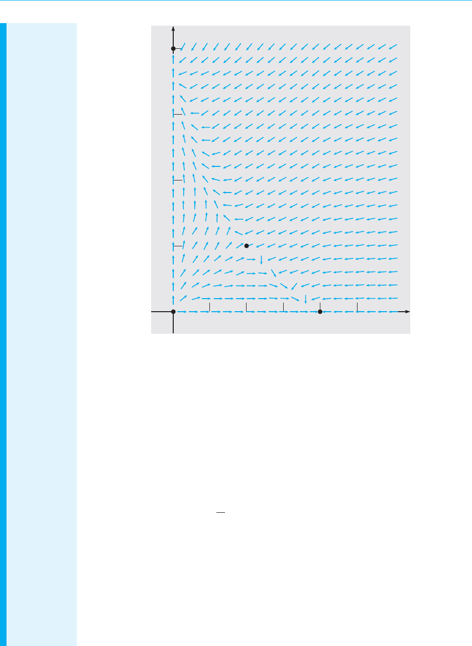
August 7, 2012 21:05 c09 Sheet number 43 Page number 537 cyan black
9.4 Competing Species 537
2
1.5
1
0.5
0
y
x
1.2510.750.50.25
FIGURE 9.4.3 Critical points and direction field for the system (20).
so the general solution is
#
x
y
$
= c
1
#
1
0
$
e
t
+ c
2
#
0
1
$
e
0.5t
. (24)
Therefore, the origin is an unstable node of the linear system (22) and also of the nonlinear
system (20). All trajectories leave the neighborhood of the origin tangent to the y-axis except
for one trajectory that lies along the x-axis.
x = 1, y = 0. The corresponding linear system is
d
dt
#
u
v
$
=
#
−1 −1
0 −0.25
$#
u
v
$
. (25)
Its eigenvalues and eigenvectors are
r
1
=−1, ξ
(1)
=
#
1
0
$
; r
2
=−0.25, ξ
(2)
=
#
4
−3
$
, (26)
and its general solution is
#
u
v
$
= c
1
#
1
0
$
e
−t
+ c
2
#
4
−3
$
e
−0.25t
. (27)

August 7, 2012 21:05 c09 Sheet number 44 Page number 538 cyan black
538 Chapter 9. Nonlinear Differential Equations and Stability
The point (1, 0) is an asymptotically stable node of the linear system (25) and of the nonlinear
system (20). If the initial values of x and y are sufficiently close to (1, 0), then the interaction
process will lead ultimately to that state—that is, to the survival of species x and the extinction
of species y. There is one pair of trajectories that approaches the critical point along the x-axis.
All other trajectories approach (1, 0) tangent to the line with slope −3/4 that is determined
by the eigenvector ξ
(2)
.
x = 0, y = 2. The analysis in this case is similar to that for the point (1, 0). The appropriate
linear system is
d
dt
#
u
v
$
=
#
−10
−1.5 −0.5
$#
u
v
$
. (28)
The eigenvalues and eigenvectors of this system are
r
1
=−1, ξ
(1)
=
#
1
3
$
; r
2
=−0.5, ξ
(2)
=
#
0
1
$
, (29)
and its general solution is
#
u
v
$
= c
1
#
1
3
$
e
−t
+ c
2
#
0
1
$
e
−0.5t
. (30)
Thus the critical point (0, 2) is an asymptotically stable node of both the linear system (28) and
the nonlinear system (20). All nearby trajectories approach the critical point tangent to the
y-axis except for one trajectory that approaches along the line with slope 3.
x = 0.5, y = 0.5. The corresponding linear system is
d
dt
#
u
v
$
=
#
−0.5 −0.5
−0.375 −0.125
$#
u
v
$
. (31)
The eigenvalues and eigenvectors are
r
1
=
−5 +
√
57
16
∼
=
0.1594, ξ
(1)
=
#
1
(−3 −
√
57)/8
$
∼
=
#
1
−1.3187
$
,
(32)
r
2
=
−5 −
√
57
16
∼
=
−0.7844, ξ
(2)
=
#
1
(−3 +
√
57)/8
$
∼
=
#
1
0.5687
$
,
so the general solution is
#
u
v
$
= c
1
#
1
−1.3187
$
e
0.1594t
+ c
2
#
1
0.5687
$
e
−0.7844t
. (33)
Since the eigenvalues are of opposite signs, the critical point (0.5, 0.5) is a saddle point and
therefore is unstable, as we had surmised earlier. All trajectories depart from the neighbor-
hood of the critical point except for one pair that approaches the saddle point as t →∞.
As they approach the critical point, the entering trajectories are tangent to the line with slope
(
√
57 − 3)/8
∼
=
0.5687 determined from the eigenvector ξ
(2)
. There is also a pair of trajectories
that approach the saddle point as t →−∞.These trajectories are tangent to the line with slope
−1.3187 corresponding to ξ
(1)
.
A phase portrait for the system (20) is shown in Figure 9.4.4. Near each of the critical
points, the trajectories of the nonlinear system behave as predicted by the corresponding
linear approximation. Of particular interest is the pair of trajectories that enter the saddle
point. These trajectories form a separatrix that divides the first quadrant into two basins of

August 7, 2012 21:05 c09 Sheet number 45 Page number 539 cyan black
9.4 Competing Species 539
attraction. Trajectories starting above the separatrix ultimately approach the node at (0, 2),
while trajectories starting below the separatrix approach the node at (1, 0). If the initial state
lies precisely on the separatrix,then the solution (x, y) will approach the saddle point as t →∞.
However, the slightest perturbation of the point (x, y) as it follows this trajectory will dislodge
the point from the separatrix and cause it to approach one of the nodes instead. Thus, in
practice, one species will survive the competition and the other will not.
y
2
1.5
1
0.5
x
Separatrix
1.2510.750.50.25
FIGURE 9.4.4 A phase portrait of the system (20). The black curve is the separatrix.
Examples 1 and 2 show that in some cases the competition between two species
leads to an equilibrium state of coexistence, while in other cases the competition
results in the eventual extinction of one of the species. To understand more clearly
how and why this happens, and to learn how to predict which situation will occur,it is
useful to look again at the general system (2). There are four cases to be considered,
depending on the relative orientation of the lines
ϵ
1
− σ
1
x − α
1
y = 0 and ϵ
2
− σ
2
y − α
2
x = 0, (34)
as shown in Figure 9.4.5. These lines are called the x- and y-nullclines, respectively,
because x
′
is zero on the first and y
′
is zero on the second. In each part of Figure 9.4.5,
the x-nullcline is the solid line and the y-nullcline is the dashed line.
Let (X , Y) denote any critical point in any one of the four cases. As in Examples
1 and 2, the system (2) is locally linear in the neighborhood of this point because the
right side of each differential equation is a quadratic polynomial. To study the system

August 7, 2012 21:05 c09 Sheet number 46 Page number 540 cyan black
540 Chapter 9. Nonlinear Differential Equations and Stability
y
x
1
/
1
σ
(a)
2
/
2
σ
1
/
1
α
2
/
2
α
y
x
(b)
1
/
1
α
2
/
2
σ
2
/
2
α
1
/
1
σ
y
x
(c)
1
/
1
σ
2
/
2
α
2
/
2
σ
1
/
1
α
y
x
(d)
1
/
1
α
2
/
2
σ
1
/
1
σ
2
/
2
α
FIGURE 9.4.5 The various cases for the competing-species system (2). The x-nullcline is
the solid line, and the y-nullcline is the dashed line.
(2) in the neighborhood of this critical point, we can look at the corresponding linear
system obtained from Eq. (13) of Section 9.3:
d
dt
'
u
v
(
=
'
ϵ
1
− 2σ
1
X − α
1
Y −α
1
X
−α
2
Y ϵ
2
− 2σ
2
Y − α
2
X
('
u
v
(
. (35)
We now use Eq. (35) to determine the conditions under which the model described
by Eqs. (2) permits the coexistence of the two species x and y. Of the four possible
cases shown in Figure 9.4.5, coexistence is possible only in cases (c) and (d). In these
cases, the nonzero values of X and Y are obtained by solving the algebraic equations
(34); the result is
X =
ϵ
1
σ
2
− ϵ
2
α
1
σ
1
σ
2
− α
1
α
2
, Y =
ϵ
2
σ
1
− ϵ
1
α
2
σ
1
σ
2
− α
1
α
2
. (36)
Further, since ϵ
1
− σ
1
X − α
1
Y = 0 and ϵ
2
− σ
2
Y − α
2
X = 0, Eq. (35) immediately
reduces to
d
dt
'
u
v
(
=
'
−σ
1
X −α
1
X
−α
2
Y −σ
2
Y
('
u
v
(
. (37)
The eigenvalues of the system (37) are found from the equation
r
2
+ (σ
1
X + σ
2
Y)r + (σ
1
σ
2
− α
1
α
2
)XY = 0. (38)

August 7, 2012 21:05 c09 Sheet number 47 Page number 541 cyan black
9.4 Competing Species 541
Thus
r
1,2
=
−(σ
1
X + σ
2
Y) ±
!
(σ
1
X + σ
2
Y)
2
− 4(σ
1
σ
2
− α
1
α
2
)XY
2
. (39)
If σ
1
σ
2
− α
1
α
2
< 0, then the radicand of Eq. (39) is positive and greater than
(σ
1
X + σ
2
Y)
2
. Thus the eigenvalues are real and opposite in sign. Consequently,
the critical point (X , Y) is an (unstable) saddle point, and coexistence is not pos-
sible. This is the case in Example 2, where σ
1
= 1, α
1
= 1, σ
2
= 0.25, α
2
= 0.75, and
σ
1
σ
2
− α
1
α
2
=−0.5.
On the other hand, if σ
1
σ
2
− α
1
α
2
> 0, then the radicand of Eq. (39) is less than
(σ
1
X + σ
2
Y)
2
. Thus the eigenvalues are real, negative, and unequal, or complex with
negative real part. A straightforward analysis of the radicand of Eq. (39) shows that
the eigenvalues cannot be complex (see Problem 7). Thus the critical point is an
asymptotically stable node, and sustained coexistence is possible. This is illustrated
by Example 1, where σ
1
= 1, α
1
= 1, σ
2
= 1, α
2
= 0.5, and σ
1
σ
2
− α
1
α
2
= 0.5.
Let us relate this result to Figures 9.4.5c and 9.4.5d. In Figure 9.4.5c we have
ϵ
1
σ
1
>
ϵ
2
α
2
or ϵ
1
α
2
>ϵ
2
σ
1
and
ϵ
2
σ
2
>
ϵ
1
α
1
or ϵ
2
α
1
>ϵ
1
σ
2
. (40)
These inequalities, coupled with the condition that X and Y given by Eqs. (36) be
positive, yield the inequality σ
1
σ
2
<α
1
α
2
. Hence in this case the critical point is a
saddle point. On the other hand, in Figure 9.4.5d we have
ϵ
1
σ
1
<
ϵ
2
α
2
or ϵ
1
α
2
<ϵ
2
σ
1
and
ϵ
2
σ
2
<
ϵ
1
α
1
or ϵ
2
α
1
<ϵ
1
σ
2
. (41)
Now the condition that X and Y be positive yields σ
1
σ
2
>α
1
α
2
. Hence the critical
point is asymptotically stable. For this case we can also show that the other
critical points (0, 0), (ϵ
1
/σ
1
,0), and (0, ϵ
2
/σ
2
) are unstable.Thus for any positive initial
values of x and y, the two populations approach the equilibrium state of coexistence
given by Eqs. (36).
Equations (2) provide the biological interpretation of the result that whether coex-
istence occurs depends on whether σ
1
σ
2
− α
1
α
2
is positive or negative. The σ’s are
a measure of the inhibitory effect that the growth of each population has on itself,
whereas the α’s are a measure of the inhibiting effect that the growth of each popu-
lation has on the other species. Thus, when σ
1
σ
2
>α
1
α
2
, interaction (competition) is
“weak” and the species can coexist; when σ
1
σ
2
<α
1
α
2
, interaction (competition)
is “strong” and the species cannot coexist—one must die out.
PROBLEMS Each of Problems 1 through 6 can be interpreted as describing the interaction of two species
with populations x and y. In each of these problems, carry out the following steps.
(a) Draw a direction field and describe how solutions seem to behave.
(b) Find the critical points.
(c) For each critical point find the corresponding linear system. Find the eigenvalues and
eigenvectors of the linear system; classify each critical point as to type,and determine whether
it is asymptotically stable, stable, or unstable.
(d) Sketch the trajectories in the neighborhood of each critical point.

August 7, 2012 21:05 c09 Sheet number 48 Page number 542 cyan black
542 Chapter 9. Nonlinear Differential Equations and Stability
(e) Compute and plot enough trajectories of the given system to show clearly the behavior of
the solutions.
(f) Determine the limiting behavior of x and y as t →∞, and interpret the results in terms
of the populations of the two species.
1.
dx/dt = x(1.5 − x − 0.5y)
dy/dt = y(2 − y − 0.75x)
2. dx/dt = x(1.5 − x − 0.5y)
dy/dt = y(2 − 0.5y − 1.5x)
3.
dx/dt = x(1.5 − 0.5x − y)
dy/dt = y(2 − y − 1.125x )
4. dx/dt = x(1.5 − 0.5x − y)
dy/dt = y(0.75 − y − 0.125x)
5.
dx/dt = x(1 − x − y)
dy/dt = y(1.5 − y − x)
6. dx/dt = x(1 − x + 0.5y)
dy/dt = y(2.5 − 1.5y + 0.25x)
7. Consider the eigenvalues given by Eq. (39) in the text. Show that
(σ
1
X + σ
2
Y)
2
− 4(σ
1
σ
2
− α
1
α
2
)XY = (σ
1
X − σ
2
Y)
2
+ 4α
1
α
2
XY.
Hence conclude that the eigenvalues can never be complex.
8. Two species of fish that compete with each other for food, but do not prey on each other,
are bluegill and redear. Suppose that a pond is stocked with bluegill and redear, and let
x and y be the populations of bluegill and redear, respectively, at time t. Suppose further
that the competition is modeled by the equations
dx/dt = x(ϵ
1
− σ
1
x − α
1
y),
dy/dt = y(ϵ
2
− σ
2
y − α
2
x).
(a) If ϵ
2
/α
2
>ϵ
1
/σ
1
and ϵ
2
/σ
2
>ϵ
1
/α
1
, show that the only equilibrium populations in the
pond are no fish, no redear, or no bluegill. What will happen for large t?
(b) If ϵ
1
/σ
1
>ϵ
2
/α
2
and ϵ
1
/α
1
>ϵ
2
/σ
2
, show that the only equilibrium populations in the
pond are no fish, no redear, or no bluegill. What will happen for large t?
9. Consider the competition between bluegill and redear mentioned in Problem 8. Suppose
that ϵ
2
/α
2
>ϵ
1
/σ
1
and ϵ
1
/α
1
>ϵ
2
/σ
2
, so,as shown in the text, there is a stable equilibrium
point at which both species can coexist. It is convenient to rewrite the equationsof Problem
8 in terms of the carrying capacity of the pond for bluegill (B = ϵ
1
/σ
1
) in the absence of
redear and its carrying capacity for redear (R = ϵ
2
/σ
2
) in the absence of bluegill.
(a) Show that the equations of Problem 8 take the form
dx
dt
= ϵ
1
x
'
1 −
1
B
x −
γ
1
B
y
(
,
dy
dt
= ϵ
2
y
'
1 −
1
R
y −
γ
2
R
x
(
,
where γ
1
= α
1
/σ
1
and γ
2
= α
2
/σ
2
. Determine the coexistence equilibrium point (X, Y) in
terms of B, R, γ
1
, and γ
2
.
(b) Now suppose that an angler fishes only for bluegill with the effect that B is reduced.
What effect does this have on the equilibrium populations? Is it possible, by fishing, to
reduce the population of bluegill to such a level that they will die out?
10. Consider the system (2) in the text, and assume that σ
1
σ
2
− α
1
α
2
= 0.
(a) Find all the critical points of the system. Observe that the result depends on whether
σ
1
ϵ
2
− α
2
ϵ
1
is zero.
(b) If σ
1
ϵ
2
− α
2
ϵ
1
> 0, classify each critical point and determine whether it is asymptoti-
cally stable, stable, or unstable. Note that Problem 5 is of this type. Then do the same if
σ
1
ϵ
2
− α
2
ϵ
1
< 0.
(c) Analyze the nature of the trajectories when σ
1
ϵ
2
− α
2
ϵ
1
= 0.

August 7, 2012 21:05 c09 Sheet number 49 Page number 543 cyan black
9.4 Competing Species 543
11. Consider the system (3) in Example 1 of the text. Recall that this system has an asymptot-
ically stable critical point at (0.5, 0.5), corresponding to the stable coexistence of the two
population species. Now suppose that immigration or emigration occurs at the constant
rates of δa and δb for the species x and y, respectively. In this case Eqs. (3) are replaced by
dx/dt = x(1 − x − y) + δa,
(i)
dy/dt = y(0.75 − y − 0.5x) + δb.
The question is what effect this has on the location of the stable equilibrium point.
(a) To find the new critical point, we must solve the equations
x(1 − x − y) + δa = 0,
(ii)
y(0.75 − y − 0.5x) + δb = 0.
One way to proceed is to assume that x and y are given by power series in the parameter
δ; thus
x = x
0
+ x
1
δ +···, y = y
0
+ y
1
δ +···. (iii)
Substitute Eqs. (iii) into Eqs. (ii) and collect terms according to powers of δ.
(b) From the constant terms (the terms not involving δ), show that x
0
= 0.5 and y
0
= 0.5,
thus confirming that in the absence of immigration or emigration, the critical point is
(0.5, 0.5).
(c) From the terms that are linear in δ, show that
x
1
= 4a − 4b, y
1
=−2a + 4b. (iv)
(d) Suppose that a > 0 and b > 0 so that immigration occurs for both species. Show that
the resulting equilibrium solution may represent an increase in both populations, or an
increase in one but a decrease in the other. Explain intuitively why this is a reasonable
result.
12.
The system
x
′
=−y, y
′
=−γy − x(x − 0.15)(x − 2)
results from an approximation to the Hodgkin–Huxley
5
equations, which model the
transmission of neural impulses along an axon.
(a) Find the critical points, and classify them by investigating the approximate linear
system near each one.
(b) Draw phase portraits for γ = 0.8 and for γ = 1.5.
(c) Consider the trajectory that leaves the critical point (2, 0). Find the value of γ for
which this trajectory ultimately approaches the origin as t →∞. Draw a phase portrait
for this value of γ.
Bifurcation Points. Consider the system
x
′
= F(x, y, α), y
′
= G(x, y, α), (i)
where α is a parameter. The equations
F(x, y, α) = 0, G(x, y, α) = 0 (ii)
5
Sir Alan L. Hodgkin (1914–1998) and Sir Andrew F. Huxley (1917– ), British physiologists and bio-
physicists, studied the excitation and transmission of neural impulses at Cambridge University and the
Marine Biological Association Laboratory in Plymouth. This work was both theoretical (resulting in a
system of nonlinear differential equations) and experimental (involving measurements on the giant axon
of the Atlantic squid). They were awarded the Nobel Prize in Physiology or Medicine in 1963.

August 7, 2012 21:05 c09 Sheet number 50 Page number 544 cyan black
544 Chapter 9. Nonlinear Differential Equations and Stability
determine the x- and y-nullclines, respectively; any point where an x-nullcline and a
y-nullcline intersect is a critical point. As α varies and the configuration of the nullclines
changes, it may well happen that, at a certain value of α, two critical points coalesce into one.
For further variation in α, the critical point may once again separate into two critical points,
or it may disappear altogether. Or the process may occur in reverse: For a certain value of α,
two formerly nonintersecting nullclines may come together, creating a critical point, which,
for further changes in α, may split into two. A value of α at which such phenomena occur is
a bifurcation point. It is also common for a critical point to experience a change in its type
and stability properties at a bifurcation point. Thus both the number and the kind of critical
points may change abruptly as α passes through a bifurcation point. Since a phase portrait of a
system is very dependent on the location and nature of the critical points, an understanding of
bifurcations is essential to an understanding of the global behavior of the system’s solutions.
In each of Problems 13 through 16:
(a) Sketch the nullclines and describe how the critical points move as α increases.
(b) Find the critical points.
(c) Let α = 2. Classify each critical point by investigating the corresponding approximate
linear system. Draw a phase portrait in a rectangle containing the critical points.
(d) Find the bifurcation point α
0
at which the critical points coincide. Locate this critical point,
and find the eigenvalues of the approximate linear system. Draw a phase portrait.
(e) For α>α
0
there are no critical points. Choose such a value of α and draw a phase portrait.
13.
x
′
=−4x + y + x
2
, y
′
=
3
2
α − y
14.
x
′
=
3
2
α − y, y
′
=−4x + y + x
2
15. x
′
=−4x + y + x
2
, y
′
=−α − x + y
16.
x
′
=−α − x + y, y
′
=−4x + y + x
2
Problems 17 through 19 deal with competitive systems much like those in Examples 1 and 2,
except that some coefficients depend on a parameter α. In each of these problems,assume that
x, y, and α are always nonnegative. In each of Problems 17 through 19:
(a) Sketch the nullclines in the first quadrant, as in Figure 9.4.5. For different ranges of α your
sketch may resemble different parts of Figure 9.4.5.
(b) Find the critical points.
(c) Determine the bifurcation points.
(d) Find the Jacobian matrix J, and evaluate it for each of the critical points.
(e) Determine the type and stability property of each critical point. Pay particular attention
to what happens as α passes through a bifurcation point.
(f) Draw phase portraits for the system for selected values of α to confirm your conclusions.
17. dx/dt = x(1 − x − y), dy/dt = y(α − y − 0.5x)
18. dx/dt = x(1 − x − y), dy/dt = y(0.75 − αy − 0.5x )
19. dx/dt = x(1 − x − y), dy/dt = y[α − y − (2α − 1)x]
9.5 Predator–Prey Equations
In the preceding section we discussed a model of two species that interact by
competing for a common food supply or other natural resource. In this section we

August 7, 2012 21:05 c09 Sheet number 51 Page number 545 cyan black
9.5 Predator–Prey Equations 545
investigate the situation inwhich one species (thepredator) preys on theother species
(the prey), while the prey lives on a different source of food. For example, consider
foxes and rabbits in a closed forest. The foxes prey on the rabbits, the rabbits live
on the vegetation in the forest. Other examples are bass in a lake as predators and
redear as prey, and ladybugs as predators and aphids as prey. We emphasize again
that a model involving only two species cannot fully describe the complex relation-
ships among species that actually occur in nature. Nevertheless, the study of simple
models is the first step toward an understanding of more complicated phenomena.
We will denote by x and y the populations of the prey and predator, respectively,
at time t. In constructing a model of the interaction of the two species, we make the
following assumptions:
1. In the absence of the predator, the prey grows at a rate proportional to the current
population; thus dx/dt = ax, a > 0, when y = 0.
2. In the absence of the prey, the predator dies out; thus dy/dt =−cy, c > 0, when x = 0.
3. The number of encounters between predator and prey is proportional to the product
of their populations. Each such encounter tends to promote the growth of the predator
and to inhibit the growth of the prey. Thus the growth rate of the predator is increased by
a term of the form γxy, while the growth rate of the prey is decreased by a term −αxy,
where γ and α are positive constants.
As a consequence of these assumptions, we are led to the equations
dx/dt = ax − αxy = x(a − αy),
(1)
dy/dt =−cy + γxy = y(−c + γx).
The constants a, c, α, and γ are all positive; a and c are the growth rate of the prey
and the death rate of the predator,respectively,and α and γ are measures of the effect
of the interaction between the two species. Equations (1) are known as the Lotka–
Volterra equations.Theywere developed inpapers byLotka
6
in 1925 and byVolterra
7
in 1926.Although these are rather simple equations, they do characterize a wide class
of problems. Ways of making them more realistic are discussed at the end of this
section and in the problems. Our goal here is to determine the qualitative behavior
of the solutions (trajectories) of the system (1) for arbitrary positive initial values of x
and y. We first do this for a specific example and then return to the general equations
(1) at the end of the section.
6
Alfred J. Lotka (1880–1949),anAmericanbiophysicist,was born in what is now Ukraine and was educated
mainly in Europe. He is remembered chiefly for his formulation of the Lotka–Volterra equations. He was
also the author, in 1924, of the first book on mathematical biology; it is now available as Elements of
Mathematical Biology (New York: Dover, 1956).
7
Vito Volterra (1860–1940), a distinguished Italian mathematician, held professorships at Pisa, Turin,
and Rome. He is particularly famous for his work in integral equations and functional analysis. Indeed,
one of the major classes of integral equations is named for him; see Problem 21 of Section 6.6. His theory
of interacting species was motivated by data collected by a friend, D’Ancona, concerning fish catches
in the Adriatic Sea. A translation of his 1926 paper can be found in an appendix to R. N. Chapman,
Animal Ecology with Special Reference to Insects (New York: McGraw-Hill, 1931).

August 7, 2012 21:05 c09 Sheet number 52 Page number 546 cyan black
546 Chapter 9. Nonlinear Differential Equations and Stability
EXAMPLE
1
Discuss the solutions of the system
dx/dt = x(1 − 0.5y) = x − 0.5xy = F(x, y),
(2)
dy/dt = y(−0.75 + 0.25x) =−0.75y + 0.25xy = G(x, y)
for x and y positive.
The critical points of this system are the solutions of the algebraic equations
x(1 − 0.5y) = 0, y(−0.75 + 0.25x) = 0, (3)
namely, the points (0, 0) and (3, 2).
Figure 9.5.1 shows the critical points and a direction field
for
the system (2). From this figure it appears that trajectories in the first quadrant encircle the
critical point (3, 2). Whether the trajectories are actually closed curves, or whether they slowly
spiral in or out, cannot be definitely determined from the direction field. The origin appears to
be a saddle point. Just as for the competition equations in Section 9.4, the coordinate axes are
trajectories of Eqs. (1) or (2). Consequently, no other trajectory can cross a coordinate axis,
which means that every solution starting in the first quadrant remains there for all time.
5
4
3
2
1
7654321
0
y
x
FIGURE 9.5.1 Critical points and direction field for the predator–prey system (2).
Next we examine the local behavior of solutions near each critical point. Near the origin
we can neglect the nonlinear terms in Eqs. (2) to obtain the corresponding linear system
d
dt
#
x
y
$
=
#
10
0 −0.75
$#
x
y
$
. (4)
The eigenvalues and eigenvectors of Eq. (4) are
r
1
= 1, ξ
(1)
=
#
1
0
$
; r
2
=−0.75, ξ
(2)
=
#
0
1
$
, (5)
so its general solution is
#
x
y
$
= c
1
#
1
0
$
e
t
+ c
2
#
0
1
$
e
−0.75t
. (6)

August 7, 2012 21:05 c09 Sheet number 53 Page number 547 cyan black
9.5 Predator–Prey Equations 547
Thus the origin is a saddle point both of the linear system (4) and of the nonlinear system (2)
and therefore is unstable. One pair of trajectories enters the origin along the y-axis; all other
trajectories depart from the neighborhood of the origin.
To examine the critical point (3, 2), we can use the Jacobian matrix
J =
#
F
x
(x, y) F
y
(x, y)
G
x
(x, y) G
y
(x, y)
$
=
#
1 − 0.5y −0.5x
0.25y −0.75 + 0.25x
$
. (7)
Evaluating J at the point (3, 2), we obtain the linear system
d
dt
#
u
v
$
=
#
0 −1.5
0.50
$#
u
v
$
, (8)
where u = x − 3 and v = y − 2. The eigenvalues and eigenvectors of this system are
r
1
=
√
3 i
2
, ξ
(1)
=
'
1
−i/
√
3
(
; r
2
=−
√
3 i
2
, ξ
(2)
=
#
1
i/
√
3
$
. (9)
Since the eigenvalues are imaginary, the critical point (3, 2) is a center of the linear system
(8) and is therefore a stable critical point for that system. Recall from Section 9.3 that this
is one of the cases in which the behavior of the linear system may or may not carry over to
the nonlinear system, so the nature of the point (3, 2) for the nonlinear system (2) cannot be
determined from this information.
The simplest way to find the trajectories of the linear system (8) is to divide the second of
Eqs. (8) by the first so as to obtain the differential equation
dv
du
=
dv/dt
du/dt
=
0.5u
−1.5v
=−
u
3v
,
or
udu+ 3v dv = 0. (10)
Consequently,
u
2
+ 3v
2
= k, (11)
where k is an arbitrary nonnegative constant of integration. Thus the trajectories of the linear
system (8) are ellipses centered at the critical point and elongated somewhat in the horizontal
direction.
Now let us return to the nonlinear system (2). Dividing the second of Eqs. (2) by the first,
we obtain
dy
dx
=
y(−0.75 + 0.25x)
x(1 − 0.5y)
. (12)
Equation (12) is a separable equation and can be put in the form
1 − 0.5y
y
dy =
−0.75 + 0.25x
x
dx,
from which it follows that
0.75 ln x + ln y − 0.5y − 0.25x = c, (13)
where c is a constant of integration. Although by using only elementary functions we cannot
solve Eq. (13) explicitly for either variable in terms of the other, it is possible to show that the
graph of the equation for a fixed value of c is a closed curve surrounding the critical point
(3, 2). Thus the critical point is also a center of the nonlinear system (2), and the predator and
prey populations exhibit a cyclic variation.

August 7, 2012 21:05 c09 Sheet number 54 Page number 548 cyan black
548 Chapter 9. Nonlinear Differential Equations and Stability
Figure 9.5.2 shows a phase portrait of the system (2). For some initial conditions, the tra-
jectory represents small variations in x and y about the critical point and is almost elliptical
in shape, as the linear analysis suggests. For other initial conditions, the oscillations in x and y
are more pronounced, and the shape of the trajectory is significantly different from an ellipse.
Observe that the trajectories are traversed in the counterclockwise direction.The dependence
of x and y on t for a typical set of initial conditions is shown in Figure 9.5.3. Note that x and
y are periodic functions of t, as they must be since the trajectories are closed curves. Fur-
ther, the oscillation of the predator population lags behind that of the prey. Starting from a
state in which both predator and prey populations are relatively small, the prey first increase
because there is little predation. Then the predators, with abundant food, increase in pop-
ulation also. This causes heavier predation, and the prey tend to decrease. Finally, with a
diminished food supply, the predator population also decreases, and the system returns to the
original state.
y
4
3
2
1
2467135
x
FIGURE 9.5.2 A phase portrait of the system (2).
x
, y
4
6
2
5 10 15 20 25
t
Prey
x(t)
Predator
y(t)
FIGURE 9.5.3 Variations of the prey and predator populations with time for the system (2).

August 7, 2012 21:05 c09 Sheet number 55 Page number 549 cyan black
9.5 Predator–Prey Equations 549
The general system (1) can be analyzed in exactly the same way as in the example.
The critical points of the system (1) are the solutions of
x(a − αy) = 0, y(−c + γx) = 0,
that is, the points (0, 0) and (c/γ, a/α). We first examine the solutions of the
corresponding linear system near each critical point.
In the neighborhood of the origin, the corresponding linear system is
d
dt
'
x
y
(
=
'
a 0
0 −c
('
x
y
(
. (14)
The eigenvalues and eigenvectors are
r
1
= a, ξ
(1)
=
'
1
0
(
; r
2
=−c , ξ
(2)
=
'
0
1
(
, (15)
so the general solution is
'
x
y
(
= c
1
'
1
0
(
e
at
+ c
2
'
0
1
(
e
−ct
. (16)
Thus the origin is a saddle point and hence unstable. Entrance to the saddle point is
along the y-axis; all other trajectories depart from the neighborhood of the critical
point.
Next consider the critical point (c/γ, a/α). The Jacobian matrix is
J =
#
a − αy −αx
γy −c + γx
$
.
Evaluating J at (c/γ, a/α), we obtain the approximate linear system
d
dt
'
u
v
(
=
'
0 −αc/γ
γa/α 0
('
u
v
(
, (17)
where u = x − (c/γ) and v = y − (a/α). The eigenvalues of the system (17) are
r =±i
√
ac, so the critical point is a (stable) center of the linear system. To find
the trajectories of the system (17), we can divide the second equation by the first to
obtain
d v
du
=
d v/dt
du/dt
=−
(γa/α)u
(αc/γ)v
, (18)
or
γ
2
au du + α
2
cv dv = 0. (19)
Consequently,
γ
2
au
2
+ α
2
cv
2
= k, (20)
where k is a nonnegative constant of integration. Thus the trajectories of the linear
system (17) are ellipses, just as in the example.
Returning briefly to the nonlinear system (1),observe that it can be reduced to the
single equation
dy
dx
=
dy/dt
dx/dt
=
y(−c + γx)
x(a − αy)
. (21)

August 7, 2012 21:05 c09 Sheet number 56 Page number 550 cyan black
550 Chapter 9. Nonlinear Differential Equations and Stability
Equation (21) is separable and has the solution
a ln y − αy + c ln x − γx = C, (22)
where C is a constant of integration. Again, it is possible to show that for fixed C, the
graph of Eq. (22) is a closed curve surrounding the critical point (c/γ, a/α). Thus this
critical point is also a center for the general nonlinear system (1).
The cyclic variation of the predator and prey populations can be analyzed in more
detail when the deviations from the point (c/γ, a/α) are small and the linear system
(17) can be used. The solution of the system (17) can be written in the form
u =
c
γ
K cos(
√
ac t + φ), v =
a
α
:
c
a
K sin(
√
ac t + φ), (23)
where the constants K and φ are determined by the initial conditions. Thus
x =
c
γ
+
c
γ
K cos(
√
ac t + φ),
(24)
y =
a
α
+
a
α
:
c
a
K sin(
√
ac t + φ).
These equations are good approximations for the nearly elliptical trajectories close
to the critical point (c/γ, a/α). We can use them to draw several conclusions about
the cyclic variation of the predator and prey on such trajectories.
1. The sizes of the predator and prey populations vary sinusoidally with period 2π/
√
ac. This
period of oscillation is independent of the initial conditions.
2. The predator and prey populations are out of phase by one-quarter of a cycle. The prey
leads and the predator lags, as explained in the example.
3. The amplitudes of the oscillations are Kc/γ for the prey and a
√
cK/α
√
a for the predator
and hence depend on the initial conditions as well as on the parameters of the problem.
4. The average populations of predator and prey over one complete cycle are c/γ and a/α,
respectively. These are the same as the equilibrium populations; see Problem 10.
Cyclic variations of predator and prey as predicted by Eqs. (1) have been observed
in nature. One striking example is described by Odum (pp. 191–192); based on the
records of the Hudson’s Bay Company of Canada, the abundance of lynx and snow-
shoe hare, as indicated by the number of pelts turned in over the period 1845–1935,
shows a distinct periodic variation with period of 9 to 10 years. The peaks of abun-
dance are followed by very rapid declines, and the peaks of abundance of the lynx
and hare are out of phase, with that of the hare preceding that of the lynx by a year
or more.
Since the critical point (c/γ, a/α) is a center, we expect that small perturbations
of the Lotka–Volterra equations may well lead to solutions that are not periodic.
To put it another way, unless the Lotka–Volterra equations exactly describe a given
predator–prey relationship, the actual fluctuations of the populations may differ
substantially from those predicted by the Lotka-Volterra equations, due to small
inaccuracies in the model equations. This has led to many attempts
8
to replace the
8
See the book by Brauer and Castillo-Chávez listed in the references for an extensive discussion of
alternative models for predator–prey relationships.

August 7, 2012 21:05 c09 Sheet number 57 Page number 551 cyan black
9.5 Predator–Prey Equations 551
Lotka–Volterra equations by other systems that are less susceptible to the effects of
small perturbations. Problem 13 introduces one such alternative model.
Another criticism of the Lotka–Volterra equations is that in the absence of
the predator, the prey will grow without bound. This can be corrected by allow-
ing for the natural inhibiting effect that an increasing population has on the growth
rate of that population. For example, the first of Eqs. (1) can be modified so that
when y = 0, it reduces to a logistic equation for x. The effects of this modification are
explored in Problems 11 and 12. Problems 14 through 16 deal with harvesting in a
predator–prey relationship. The results may seem rather counterintuitive.
Finally, we repeat a warning stated earlier: relationships among species in the
natural world are often complex and subtle. You should not expect too much of a
simple system of two differential equations in describing such relationships. Even if
you are convinced that the general form of the equations is sound, the determination
of numerical values for the coefficients may present serious difficulties.
PROBLEMS Each of Problems 1 through 5 can be interpreted as describing the interaction of two species
with population densities x and y. In each of these problems, carry out the following steps.
(a) Draw a direction field and describe how solutions seem to behave.
(b) Find the critical points.
(c) For each critical point, find the corresponding linear system. Find the eigenvalues and
eigenvectors of the linear system; classify each critical point as to type,and determine whether
it is asymptotically stable, stable, or unstable.
(d) Sketch the trajectories in the neighborhood of each critical point.
(e) Draw a phase portrait for the system.
(f) Determine the limiting behavior of x and y as t →∞, and interpret the results in terms
of the populations of the two species.
1.
dx/dt = x(1.5 − 0.5y)
dy/dt = y(−0.5 + x)
2. dx/dt = x(1 − 0.5y)
dy/dt = y(−0.25 + 0.5x)
3.
dx/dt = x(1 − 0.5x − 0.5y)
dy/dt = y(−0.25 + 0.5x)
4. dx/dt = x(1.125 − x − 0.5y)
dy/dt = y(−1 + x)
5.
dx/dt = x(−1 + 2.5x − 0.3y − x
2
)
dy/dt = y(−1.5 + x)
6. In this problem we examine the phase difference between the cyclic variations of the
predator and prey populations as given by Eqs. (24) of this section. Suppose we assume
that K > 0 and that t is measured from the time that the prey population x is a maximum;
then φ = 0.
(a) Show that the predator population y is a maximum at t = π/2
√
ac = T/4, where T is
the period of the oscillation.
(b) When is the prey population increasing most rapidly? decreasing most rapidly? a
minimum?
(c) Answer the questions in part (b) for the predator population.
(d) Draw a typical elliptic trajectory enclosing the point (c/γ, a/α), and mark on it the
points found in parts (a), (b), and (c).
7.
(a) Findthe ratio of theamplitudes of the oscillations ofthe prey and predator populations
about the critical point (c/γ, a/α), using the approximation (24), which is valid for small
oscillations. Observe that the ratio is independent of the initial conditions.

August 7, 2012 21:05 c09 Sheet number 58 Page number 552 cyan black
552 Chapter 9. Nonlinear Differential Equations and Stability
(b) Evaluate the ratio found in part (a) for the system (2).
(c) Estimate the amplitude ratio for the solution of the nonlinear system (2) shown in
Figure 9.5.3. Does the result agree with that obtained from the linear approximation?
(d) Determine the prey–predator amplitude ratio for other solutions of the system (2)
—that is, for solutions satisfying other initial conditions. Is the ratio independent of the
initial conditions?
8.
(a) Find the period of the oscillations of the prey and predator populations, using the
approximation (24), which is valid for small oscillations. Note that the period is inde-
pendent of the amplitude of the oscillations.
(b) For the solution of the nonlinear system (2) shown in Figure 9.5.3,estimate the period
as well as possible. Is the result the same as for the linear approximation?
(c) Calculate other solutions of the system (2)—that is, solutions satisfying other initial
conditions—and determine their periods. Is the period the same for all initial conditions?
9.
Consider the system
dx/dt = ax[1 − (y/2)], dy/dt = by[−1 + (x/3)],
where a and b are positive constants. Observe that this system is the same as in the example
in the text if a = 1 and b = 0.75. Suppose the initial conditions are x(0) = 5 and y(0) = 2.
(a) Let a = 1 and b = 1. Plot the trajectory in the phase plane, and determine (or esti-
mate) the period of the oscillation.
(b) Repeat part (a) for a = 3 and a = 1/3, with b = 1.
(c) Repeat part (a) for b = 3 and b = 1/3, with a = 1.
(d) Describe how the period and the shape of the trajectory depend on a and b.
10.
The average sizes of the prey and predator populations are defined as
x =
1
T
"
A+T
A
x(t) dt, y =
1
T
"
A+T
A
y(t) dt,
respectively, where T is the period of a full cycle, and A is any nonnegative constant.
(a) Using the approximation (24), which is valid near the critical point, show that
x = c/γ
and
y = a/α.
(b) For the solution of the nonlinear system (2) shown in Figure 9.5.3, estimate
x and y as
well as you can. Try to determine whether
x and y are given by c/γ and a/α, respectively,
in this case.
Hint: Consider how you might estimate the value of an integral even though you do not
have a formula for the integrand.
(c) Calculate other solutions of the system (2)—that is, solutions satisfying other initial
conditions—and determine
x and y for these solutions. Are the values of x and y the same
for all solutions?
In Problems 11 and 12, we consider the effect of modifying the equation for the prey x by
including a term −σx
2
so that this equation reduces to a logistic equation in the absence of
the predator y. Problem 11 deals with a specific system of this kind, and Problem 12 takes
up this modification to the general Lotka–Volterra system. The systems in Problems 3 and
4 are other examples of this type.
11. Consider the system
x
′
= x(1 − σx − 0.5y), y
′
= y(−0.75 + 0.25x),
where σ>0. Observe that this system is a modification of the system (2) in Example 1.

August 7, 2012 21:05 c09 Sheet number 59 Page number 553 cyan black
9.5 Predator–Prey Equations 553
(a) Find all of the critical points. How does their location change as σ increases from zero?
Observe that there is a critical point in the interior of the first quadrant only if σ<1/3.
(b) Determine the type and stability property of each critical point. Find the value
σ
1
< 1/3 where the nature of the critical point in the interior of the first quadrant changes.
Describe the change that takes place in this critical point as σ passes through σ
1
.
(c) Draw a direction field and phase portrait for a value of σ between zero and σ
1
; for a
value of σ between σ
1
and 1/3.
(d) Describe the effect on the two populations as σ increases from zero to 1/3.
12. Consider the system
dx/dt = x(a − σx − αy), dy/dt = y(−c + γx),
where a, σ, α, c, and γ are positive constants.
(a) Find all critical points of the given system. How does their location change as σ
increases from zero? Assume that a/σ > c/γ, that is, σ<aγ/c. Why is this assumption
necessary?
(b) Determine the nature and stability characteristics of each critical point.
(c) Show that there is a value of σ between zero and aγ/c where the critical point in the
interior of the first quadrant changes from a spiral point to a node.
(d) Describe the effect on the two populations as σ increases from zero to aγ/c.
13. In the Lotka–Volterra equations, the interaction between the two species is modeled by
terms proportional to the product xy of the respective populations. If the preypopulation is
much larger than the predator population,this may overstate the interaction;for example,
a predator may hunt only when it is hungry and ignore the prey at other times. In this
problem we consider an alternative model proposed by Rosenzweig and MacArthur.
9
(a) Consider the system
x
′
= x
'
1 − 0.2x −
2y
x + 6
(
, y
′
= y
'
−0.25 +
x
x + 6
(
.
Find all of the critical points of this system.
(b) Determine the type and stability characteristics of each critical point.
(c) Draw a direction field and phase portrait for this system.
Harvesting in a Predator–Prey Relationship. In a predator–prey situation,it may happen
that one or perhaps both species are valuable sources of food. Or, the prey species may
be regarded as a pest, leading to efforts to reduce its numbers. In a constant-effort model
of harvesting, we introduce a term −E
1
x in the prey equation and a term −E
2
y in the
predator equation, where E
1
and E
2
are measures of the effort invested in harvesting
the respective species. A constant-yield model of harvesting is obtained by including the
term −H
1
in the prey equation and the term −H
2
in the predator equation. The constants
E
1
, E
2
, H
1
, and H
2
are always nonnegative. Problems 14 and 15 deal with constant-effort
harvesting, and Problem 16 deals with constant-yield harvesting.
14. Applying a constant-effort model of harvesting to the Lotka–Volterra equations (1), we
obtain the system
x
′
= x(a − αy − E
1
), y
′
= y(−c + γx − E
2
).
When there is no harvesting, the equilibrium solution is (c/γ, a/α).
9
See the book by Brauer and Castillo-Chávez for further details.

August 7, 2012 21:05 c09 Sheet number 60 Page number 554 cyan black
554 Chapter 9. Nonlinear Differential Equations and Stability
(a) Before doing any mathematical analysis, think about the situation intuitively. How do
you think the populations will change if the prey alone is harvested? if the predator alone
is harvested? if both are harvested?
(b) How does the equilibrium solution change if the prey is harvested, but not the preda-
tor (E
1
> 0, E
2
= 0)?
(c) How does the equilibrium solution change if the predator is harvested, but not the
prey (E
1
= 0, E
2
> 0)?
(d) How does the equilibrium solution change if both are harvested (E
1
> 0, E
2
> 0)?
15. If we modify the Lotka–Volterra equations by including a self-limiting term −σx
2
in the
prey equation, and then assume constant-effort harvesting, we obtain the equations
x
′
= x(a − σx − αy − E
1
), y
′
= y(−c + γx − E
2
).
In the absence of harvesting, the equilibrium solution of interest is x = c/γ,
y = (a/α) − (σc)/(αγ).
(a) How does the equilibrium solution change if the prey is harvested, but not the preda-
tor (E
1
> 0, E
2
= 0)?
(b) How does the equilibrium solution change if the predator is harvested, but not the
prey (E
1
= 0, E
2
> 0)?
(c) How does the equilibrium solution change if both are harvested (E
1
> 0, E
2
> 0)?
16. In this problem we apply a constant-yield modelof harvesting to the situation in Example 1.
Consider the system
x
′
= x(1 − 0.5y) − H
1
, y
′
= y(−0.75 + 0.25x) − H
2
,
where H
1
and H
2
are nonnegative constants. Recall that if H
1
= H
2
= 0, then (3, 2) is an
equilibrium solution for this system.
(a) Before doing any mathematical analysis, think about the situation intuitively. How do
you think the populations will change if the prey alone is harvested? if the predator alone
is harvested? if both are harvested?
(b) How does the equilibrium solution change if the prey is harvested, but not the preda-
tor (H
1
> 0, H
2
= 0)?
(c) How does the equilibrium solution change if the predator is harvested, but not the
prey (H
1
= 0, H
2
> 0)?
(d) How does the equilibrium solution change if both are harvested (H
1
> 0, H
2
> 0)?
9.6 Liapunov’s Second Method
In Section 9.3 we showed how the stability of a critical point of a locally linear
system can usually be determined from a study of the corresponding linear system.
However, no conclusion can be drawn when the critical point is a center of the
corresponding linear system. Examples of this situation are the undamped pendulum,
Eqs. (1) and (2) below, and the predator–prey problem discussed in Section 9.5. Also,
for an asymptotically stable critical point, it may be important to investigate the
basin of attraction—that is, the domain such that all solutions starting within that
domain approach the critical point. The theory of locally linear systems provides no
information about this question.

August 7, 2012 21:05 c09 Sheet number 61 Page number 555 cyan black
9.6 Liapunov’s Second Method 555
In this section we discuss another approach,known as Liapunov’s
10
second method
or direct method.The method is referred to as a direct method because no knowledge
of the solution of the system of differential equations is required. Rather,conclusions
about the stability or instability of a critical point are obtained by constructing a suit-
able auxiliary function. The technique is a very powerful one that provides a more
global type of information—for example, an estimate of the extent of the basin of
attraction of a critical point. Liapunov’s second method can also be used to study
systems of equations that are not locally linear; however, we will not discuss such
problems.
The Pendulum Equations. Basically, Liapunov’s second method is a generalization of
two physical principles for conservative systems, namely, (i) a rest position is stable
if the potential energy is a local minimum, otherwise it is unstable, and (ii) the total
energy is a constant during any motion. To illustrate these concepts, again consider
the undamped pendulum (a conservative mechanical system), which is governed
by the equation
d
2
θ
dt
2
+
g
L
sin θ = 0. (1)
The corresponding system of first order equations is
dx
dt
= y,
dy
dt
=−
g
L
sin x, (2)
where x = θ and y = dθ/dt. If we omit an arbitrary constant, the potential energy U
is the work done in lifting the pendulum above its lowest position, namely,
U(x, y) = mgL(1 − cos x); (3)
see Figure 9.2.2. The critical points of the system (2) are x =±nπ, y = 0, for
n = 0, 1,2, 3, ..., corresponding to θ =±nπ, dθ/dt = 0. Physically, we expect the
points x = 0,y = 0;x =±2π,y = 0; ...,corresponding to θ = 0, ±2π, ..., to be stable,
since for them the pendulum bob is vertical with the weight down. Further,we expect
the points x =±π, y = 0; x =±3π, y = 0; ..., corresponding to θ =±π, ±3π, ...,to
be
unstable, since for them the pendulum bob is vertical with the weight up. This
agrees with statement (i), for at the former points U is a minimum equal to zero, and
at the latter points U is a maximum equal to 2mgL.
Next consider the total energy V, which is the sum of the potential energy U and
the kinetic energy
1
2
mL
2
(d θ/dt)
2
. In terms of x and y,
V(x, y) = mgL(1 − cos x) +
1
2
mL
2
y
2
. (4)
10
Alexander M. Liapunov (1857–1918), a student of Chebyshev at St. Petersburg, taught at the Uni-
versity of Kharkov from 1885 to 1901, when he became an academician in applied mathematics at the
St. Petersburg Academy of Sciences. In 1917 he moved to Odessa because of his wife’s frail health. His
research in stability encompassed both theoretical analysis and applications to various physical problems.
His second method formed part of his most influential work, General Problem of Stability of Motion,
published in 1892.

August 7, 2012 21:05 c09 Sheet number 62 Page number 556 cyan black
556 Chapter 9. Nonlinear Differential Equations and Stability
On a trajectory corresponding to a solution x = φ(t), y = ψ(t) of Eqs. (2), V can be
considered a function of t. The derivative of V[φ(t), ψ(t)] with respect to t is called
the rate of change of V following the trajectory. By the chain rule,
dV[φ(t), ψ(t)]
dt
= V
x
[φ(t), ψ(t)]
d φ(t)
dt
+ V
y
[φ(t), ψ(t)]
d ψ(t)
dt
= (mgL sin x)
dx
dt
+ mL
2
y
dy
dt
, (5)
where it is understood that x = φ(t), y = ψ(t). Finally,substituting in Eq. (5) for dx/dt
and dy/dt from Eqs. (2), we find that dV/dt = 0. Hence V is a constant along any
trajectory of the system (2), which is statement (ii).
It is important to note that at any point (x, y), the rate of change of V along the
trajectory through that point was computed without actually solving the system (2).
It is precisely this fact that enables us to use Liapunov’s second method for systems
whose solution we do not know, which is the main reason for its importance.
At the stable critical points, x =±2nπ, y = 0, n = 0, 1, 2, ..., the energy V is zero.
If the initial state (x
1
, y
1
) of the pendulum is sufficiently near a stable critical point,
then the energy V(x
1
, y
1
) is small, and the motion (trajectory) associated with this
energy stays close to the critical point. It can be shown that if V(x
1
, y
1
) is sufficiently
small, then the trajectory is closed and contains the critical point. For example, sup-
pose that (x
1
, y
1
) is near (0, 0) and that V(x
1
, y
1
) is very small. The equation of the
trajectory with energy V(x
1
, y
1
) is
V(x, y) = mgL(1 − cos x) +
1
2
mL
2
y
2
= V(x
1
, y
1
).
For x small, we have 1 − cos x = 1 − (1 − x
2
/2!+···)
∼
=
x
2
/2. Thus the equation of
the trajectory is approximately
1
2
mgLx
2
+
1
2
mL
2
y
2
= V(x
1
, y
1
),
or
x
2
2V(x
1
, y
1
)/mgL
+
y
2
2V(x
1
, y
1
)/mL
2
= 1.
This is an ellipse enclosing the critical point (0, 0);the smaller V(x
1
, y
1
) is, the smaller
are the major and minor axes of the ellipse. Physically, the closed trajectory corre-
sponds to a solution that is periodic in time—the motion is a small oscillation about
the equilibrium point.
If damping is present, however, it is natural to expect that the amplitude of the
motion decays in time and that the stable critical point (center) becomes an asymp-
totically stable critical point (spiral point). See the phase portrait for the damped
pendulum in Figure 9.3.5. This can almost be argued from a consideration of dV/dt.
For the damped pendulum, the total energy is still given by Eq. (4), but now, from
Eqs. (13) of Section 9.2,dx /dt = y and dy/dt =−(g/L) sin x − (c/mL)y. Substituting
for dx/dt and dy/dt in Eq. (5) gives dV/dt =−cLy
2
≤ 0. Thus the energy is nonin-
creasing along any trajectory, and except for the line y = 0, the motion is such that
the energy decreases. Hence each trajectory must approach a point of minimum
energy—a stable equilibrium point. If dV/dt < 0 instead of dV/dt ≤ 0, it is reason-
able to expect that this would be true for all trajectories that start sufficiently close
to the origin.

August 7, 2012 21:05 c09 Sheet number 63 Page number 557 cyan black
9.6 Liapunov’s Second Method 557
General Systems. To pursue these ideas further, consider the autonomous system
dx/dt = F(x, y), dy/dt = G(x, y), (6)
and suppose that the point x = 0, y = 0 is an asymptotically stable critical point.
Then there exists some domain D containing (0, 0) such that every trajectory that
starts in D must approach the origin as t →∞. Suppose that there exists an“energy”
function V such that V ≥ 0 for (x, y) in D with V = 0 only at the origin. Since each
trajectory in D approaches the origin as t →∞, then following any particular trajec-
tory, V decreases to zero as t approaches infinity. The type of result we want to prove
is essentially the converse: if, on every trajectory, V decreases to zero as t increases,
then the trajectories must approach the origin as t →∞, and hence the origin is
asymptotically stable. First, however, it is necessary to make several definitions.
Let V be defined on some domain D containing the origin. Then V is said to
be positive definite on D if V(0, 0) = 0 and V(x, y)>0
for all other points in D
.
Similarly, V is said to be negative definite on D if V(0, 0) = 0 and V(x, y)<0 for all
other points in D. If the inequalities > and < are replaced by ≥ and ≤, then V is
said to be positive semidefinite and negative semidefinite,respectively.We emphasize
that when we speak of a positive definite (negative definite, …) function on a domain
D containing the origin,the functionmust bezero atthe origin in additionto satisfying
the proper inequality at all other points in D.
EXAMPLE
1
The function
V(x, y) = sin(x
2
+ y
2
)
is positive definite on x
2
+ y
2
<π/2 since V(0, 0) = 0 and V(x, y)>0 for 0 < x
2
+ y
2
<π/2.
However, the function
V(x, y) = (x + y)
2
is only positive semidefinite since V(x, y) = 0 on the line y =−x.
We also want to consider the function
˙
V(x, y) = V
x
(x, y)F(x, y) + V
y
(x, y)G(x, y), (7)
where F and G are the same functions as in Eqs. (6). We choose this notation
because
˙
V(x, y) can be identified as the rate of change of V along the trajectory
of the system (6) that passes through the point (x , y). That is, if x = φ(t), y = ψ(t) is
a solution of the system (6), then
dV[φ(t), ψ(t)]
dt
= V
x
[φ(t), ψ(t)]
d φ(t)
dt
+ V
y
[φ(t), ψ(t)]
d ψ(t)
dt
= V
x
(x, y)F(x, y) + V
y
(x, y)G(x, y)
=
˙
V(x, y). (8)
The function
˙
V is sometimes referred to as the derivative of V with respect to the
system (6).
We now state two Liapunov theorems, the first dealing with stability, the second
with instability.

August 7, 2012 21:05 c09 Sheet number 64 Page number 558 cyan black
558 Chapter 9. Nonlinear Differential Equations and Stability
Theorem 9.6.1
Suppose that the autonomous system (6) has an isolated critical point at the ori-
gin. If there exists a function V that is continuous and has continuous first partial
derivatives, that is positive definite, and for which the function
˙
V given by Eq. (7)
is negative definite on some domain D in the xy-plane containing (0, 0), then the
origin is an asymptotically stable critical point. If
˙
V is negative semidefinite, then
the origin is a stable critical point.
Theorem 9.6.2
Let the origin be an isolated critical point of the autonomous system (6). Let V be a
function that is continuous and has continuous first partial derivatives. Suppose that
V(0, 0) = 0 and that in every neighborhood of the origin there is at least one point
at which V is positive (negative). If there exists a domain D containing the origin
such that the function
˙
V given by Eq. (7) is positive definite (negative definite) on
D, then the origin is an unstable critical point.
The function V is called a Liapunov function. Before sketching geometrical argu-
ments forTheorems 9.6.1 and 9.6.2,we note that the difficulty in using these theorems
is that they tell us nothing about how to construct a Liapunov function, assuming that
one exists. In cases where the autonomous system (6) represents a physical prob-
lem, it is natural to consider first the actual total energy function of the system as
a possible Liapunov function. However, Theorems 9.6.1 and 9.6.2 are applicable in
cases where the concept of physical energy is not pertinent. In such cases a judicious
trial-and-error approach may be necessary.
Now consider the second part of Theorem 9.6.1—that is, the case
˙
V ≤ 0. Let
c ≥ 0 be a constant, and consider the curve in the xy-plane given by V(x, y) = c.
For c = 0 the curve reduces to the single point x = 0, y = 0. We assume that if
0 < c
1
< c
2
, then the curve V(x, y) = c
1
contains the origin and lies within the curve
V(x, y) = c
2
, as illustrated in Figure 9.6.1a. We show that a trajectory starting inside
a closed curve V(x , y) = c cannot cross to the outside. Thus, given a circle of radius
ϵ about the origin, by taking c sufficiently small, we can ensure that every trajectory
starting inside the closed curve V(x, y) = c stays within the circle of radius ϵ; indeed,
it stays within the closed curve V(x, y) = c itself. Thus the origin is a stable critical
point.
To show this, recall from calculus that the vector
∇V(x, y) = V
x
(x, y)i + V
y
(x, y)j, (9)
known as the gradient of V, is normal to the curve V(x, y) = c and points in the direc-
tion of increasing V. In the present case, V increases outward from the origin, so ∇V
points away from the origin, as indicated in Figure 9.6.1b. Next, consider a trajectory
x = φ(t), y = ψ(t) of the system (6), and recall that the vector T(t) = φ
′
(t)i + ψ
′
(t)j
is tangent to the trajectory at each point; see Figure 9.6.1b. Let x
1
= φ(t
1
), y
1
= ψ(t
1
)
be a point of intersection of the trajectory and a closed curve V(x, y) = c. At this
point φ
′
(t
1
) = F(x
1
, y
1
), ψ
′
(t
1
) = G(x
1
, y
1
), so from Eq. (7) we obtain
˙
V(x
1
, y
1
) = V
x
(x
1
, y
1
)φ
′
(t
1
) + V
y
(x
1
, y
1
)ψ
′
(t
1
)
=[V
x
(x
1
, y
1
)i + V
y
(x
1
, y
1
)j] · [φ
′
(t
1
)i + ψ
′
(t
1
)j]
= ∇V(x
1
, y
1
) · T(t
1
). (10)

August 7, 2012 21:05 c09 Sheet number 65 Page number 559 cyan black
9.6 Liapunov’s Second Method 559
(a)
x
y
c = 0
c
1
0 < c
1
< c
2
c
2
(b)
x
y
x = (t)
φ
y = (t)
ψ
V(x, y) = c
(x
1
, y
1
)
V
x
(x
1
, y
1
) i + V
y
(x
1
, y
1
) j = V(x
1
, y
1
)
d (t
1
)
φ
dt
d (t
1
)
ψ
dt
i + j = T(t
1
)
FIGURE 9.6.1 (a) The curves V(x, y) = c
1
and V(x, y) = c
2
with 0 < c
1
< c
2
.
(b) Geometrical interpretation of Liapunov’s second method.
Thus
˙
V(x
1
, y
1
) is the scalar product of the vector ∇V(x
1
, y
1
) and the vector
T(t
1
). Since
˙
V(x
1
, y
1
) ≤ 0, it follows that the cosine of the angle between ∇V(x
1
, y
1
)
and T(t
1
) is also less than or equal to zero; hence the angle itself is in the range
[π/2, 3π/2]. Thus the direction of motion on the trajectory is inward with respect to
V(x
1
, y
1
) = c or, at worst, tangent to this curve. Trajectories starting inside a closed
curve V(x
1
, y
1
) = c (no matter how small c is) cannot escape, so the origin is a sta-
ble point. If
˙
V(x
1
, y
1
)<0, then the trajectories passing through points on the curve
are actually pointed inward. As a consequence, it can be shown that trajectories
starting sufficiently close to the origin must approach the origin; hence the origin is
asymptotically stable.
A geometrical argument for Theorem 9.6.2 follows in a somewhat similar manner.
Briefly,suppose that
˙
V is positive definite,and suppose that given any circle about the
origin, there is an interior point (x
1
, y
1
) at which V(x
1
, y
1
)>0. Consider a trajectory
that starts at (x
1
, y
1
). It follows from Eq. (8) that along this trajectory,V must increase
since
˙
V(x
1
, y
1
)>0; furthermore, since V(x
1
, y
1
)>0, the trajectory cannot approach
the origin because V(0, 0) = 0. This shows that the origin cannot be asymptotically
stable. By further exploiting the fact that
˙
V(x, y)>0, it is possible to show that the
origin is an unstable point; however, we will not pursue this argument.
EXAMPLE
2
Use Theorem 9.6.1 to show that (0, 0) is a stable critical point for the undamped pendulum
equations (2). Also use Theorem 9.6.2 to show that (π ,0) is an unstable critical point.
Let V be the total energy given by Eq. (4):
V(x, y) = mgL(1 − cos x) +
1
2
mL
2
y
2
. (4)
If we take D to be the domain −π/2 < x <π/2, −∞ < y < ∞, then V is positive there
except at the origin, where it is zero. Thus V is positive definite on D. Further, as we have
already seen,
˙
V = (mgL sin x)(y) + (mL
2
y)(−g sin x)/L = 0
for all x and y. Thus
˙
V is negative semidefinite on D. Consequently, by the last statement
in Theorem 9.6.1, the origin is a stable critical point for the undamped pendulum. Observe
that this conclusion cannot be obtained from Theorem 9.3.2 because (0, 0) is a center for the
corresponding linear system.

August 7, 2012 21:05 c09 Sheet number 66 Page number 560 cyan black
560 Chapter 9. Nonlinear Differential Equations and Stability
Now consider the critical point (π,0). The Liapunov function given by Eq. (4) is no longer
suitable because Theorem 9.6.2 calls for a function V for which
˙
V is either positive or negative
definite. To analyze the point (π,0), it is convenient to move this point to the origin by the
change of variables x = π + u, y = v. Then the differential equations (2) become
du/dt = v, dv/dt =
g
L
sin u, (11)
and the critical point is (0, 0) in the uv-plane. Consider the function
V(u, v) = v sinu (12)
and let D be the domain −π/4 < u <π/4, −∞ <v<∞. Then
˙
V = (v cos u)(v) + (sin u)[(g/L) sin u]=v
2
cos u + (g/L) sin
2
u (13)
is positive definite in D. The only remaining question is whether there are points in every
neighborhood of the origin where V itself is positive. From Eq. (12) we see that V(u, v) > 0
in the first quadrant (where both sin u and v are positive) and in the third quadrant (where
both are negative). Thus the conditions of Theorem 9.6.2 are satisfied, and the point (0, 0) in
the uv-plane, corresponding to the point (π,0) in the xy-plane, is unstable.
The damped pendulum equations are discussed in Problem 7.
From a practical point of view, we are often interested in the basin of attraction.
The following theorem provides some information on this subject.
Theorem 9.6.3
Let the origin be an isolated critical point of the autonomous system (6). Let the
function V be continuous and have continuous first partial derivatives. If there is a
bounded domain D
K
containing the origin where V(x, y)<K for some positive K,
V is positive definite, and
˙
V is negative definite, then every solution of Eqs. (6) that
starts at a point in D
K
approaches the origin as t approaches infinity.
In other words, Theorem 9.6.3 says that if x = φ(t), y = ψ(t) is the solution of
Eqs. (6) for initial data lying in D
K
, then (x, y) approaches the critical point (0, 0) as
t →∞. Thus D
K
gives a region of asymptotic stability; of course, it may not be the
entire basin of attraction. This theorem is proved by showing that (i) there are no
periodic solutions of the system (6) in D
K
, and (ii) there are no other critical points
in D
K
. It then follows that trajectories starting in D
K
cannot escape and therefore
must tend to the origin as t tends to infinity.
Theorems 9.6.1 and 9.6.2 give sufficient conditions for stability and instability,
respectively, but these conditions are not necessary. Also, our failure to find a suit-
able Liapunov function does not mean that there is no such function. Unfortunately,
there are no general methods for the construction of Liapunov functions; how-
ever, there has been extensive work on the construction of Liapunov functions for
special classes of equations. An elementary algebraic result that is often useful in
constructing positive definite or negative definite functions is stated without proof
in the following theorem.

August 7, 2012 21:05 c09 Sheet number 67 Page number 561 cyan black
9.6 Liapunov’s Second Method 561
Theorem 9.6.4
The function
V(x, y) = ax
2
+ bxy + cy
2
(14)
is positive definite if, and only if,
a > 0 and 4 ac − b
2
> 0 (15)
and is negative definite if, and only if,
a < 0 and 4 ac − b
2
> 0. (16)
The use of Theorem 9.6.4 is illustrated in the following example.
EXAMPLE
3
Show that the critical point (0, 0) of the autonomous system
dx/dt =−x − xy
2
, dy/dt =−y − x
2
y (17)
is asymptotically stable.
We try to construct a Liapunov function of the form (14). Then V
x
(x, y) = 2 ax + by,
V
y
(x, y) = bx + 2cy, so
˙
V(x, y) = (2 ax + by)(−x − xy
2
) + (bx + 2cy)(−y − x
2
y)
=−
.
2a(x
2
+ x
2
y
2
) + b(2xy + xy
3
+ x
3
y) + 2c(y
2
+ x
2
y
2
)
/
.
If we choose b = 0, and a and c to be any positive numbers, then
˙
V is negative definite and V
is positive definite by Theorem 9.6.4. Thus, by Theorem 9.6.1, the origin is an asymptotically
stable critical point.
EXAMPLE
4
Consider the system
dx/dt = x(1 − x − y),
(18)
dy/dt = y(0.75 − y − 0.5x).
In Example 1 of Section 9.4, we found that this system models a certain pair of competing
species and that the critical point (0.5, 0.5) is asymptotically stable. Confirm this conclusion by
finding a suitable Liapunov function.
It is helpful to transform the point (0.5, 0.5) to the origin. To this end, let
x = 0.5 + u, y = 0.5 + v. (19)
Then, substituting for x and y in Eqs. (18), we obtain the new system
du/dt =−0.5u − 0.5v − u
2
− uv,
(20)
dv/dt =−0.25u − 0.5v − 0.5uv − v
2
.
To keep the calculations relatively simple,consider the function V(u, v) = u
2
+ v
2
as a possible
Liapunov function. This function is clearly positive definite, so we need only to determine

August 7, 2012 21:05 c09 Sheet number 68 Page number 562 cyan black
562 Chapter 9. Nonlinear Differential Equations and Stability
whether there is a region containing the origin in the uv-plane where the derivative
˙
V with
respect to the system (20) is negative definite. We compute
˙
V(u, v) and find that
˙
V(u, v) = V
u
du
dt
+ V
v
dv
dt
= 2u(−0.5u − 0.5v − u
2
− uv) + 2v(−0 .25u − 0.5v − 0.5uv − v
2
),
or
˙
V(u, v) =−
.
(u
2
+ 1.5uv + v
2
) + (2u
3
+ 2u
2
v + uv
2
+ 2v
3
)
/
, (21)
where we have collected together the quadratic and cubic terms. We want to show that the
expression in square brackets in Eq. (21) is positive definite, at least for u and v sufficiently
small. Observe that the quadratic terms can be written as
u
2
+ 1.5uv + v
2
= 0.25(u
2
+ v
2
) + 0.75(u + v)
2
, (22)
so these terms are positive definite. On the other hand, the cubic terms in Eq. (21) may be of
either sign. Thus we must show that, in some neighborhood of u = 0, v = 0, the cubic terms
are smaller in magnitude than the quadratic terms; that is,
3
3
2u
3
+ 2u
2
v + uv
2
+ 2v
3
3
3
< 0.25(u
2
+ v
2
) + 0.75(u + v)
2
. (23)
To estimate the left side of Eq. (23), we introduce polar coordinates u = r cos θ, v = r sin θ.
Then
3
3
2u
3
+ 2u
2
v + uv
2
+ 2v
3
3
3
= r
3
3
3
2 cos
3
θ + 2 cos
2
θ sin θ + cos θ sin
2
θ + 2 sin
3
θ
3
3
≤ r
3
.
2|cos
3
θ|+2 cos
2
θ|sin θ|+|cos θ|sin
2
θ + 2|sin
3
θ|
/
≤ 7r
3
,
since |sin θ|, |cos θ|≤1. To satisfy Eq. (23), it is now certainly sufficient to satisfy the more
stringent requirement
7r
3
< 0.25(u
2
+ v
2
) = 0.25r
2
=
1
4
r
2
,
which yields r < 1/28. Thus, at least in this disk, the hypotheses of Theorem 9.6.1 are satisfied,
so the origin is an asymptotically stable critical point of the system (20). The same is then true
of the critical point (0.5, 0.5) of the original system (18).
If we refer to Theorem 9.6.3, the preceding argument also shows that the disk with center
(0.5, 0.5) and radius 1/28 is a region of asymptotic stability for the system (18). This is a
severe underestimate of the full basin of attraction, as the discussion in Section 9.4 shows.
To obtain a better estimate of the actual basin of attraction from Theorem 9.6.3, we would
have to estimate the terms in Eq. (23) more accurately, or use a better (and presumably more
complicated) Liapunov function, or both.
PROBLEMS In each of Problems 1 through 4, construct a suitable Liapunov function of the form ax
2
+ cy
2
,
where a and c are to be determined. Then show that the critical point at the origin is of the
indicated type.
1. dx/dt =−x
3
+ xy
2
, dy/dt =−2x
2
y − y
3
; asymptotically stable
2. dx/dt =−
1
2
x
3
+ 2xy
2
, dy/dt =−y
3
; asymptotically stable
3. dx/dt =−x
3
+ 2y
3
, dy/dt =−2xy
2
; stable (at least)
4. dx/dt = x
3
− y
3
, dy/dt = 2xy
2
+ 4x
2
y + 2y
3
; unstable

August 7, 2012 21:05 c09 Sheet number 69 Page number 563 cyan black
9.6 Liapunov’s Second Method 563
5. Consider the system of equations
dx/dt = y − xf (x, y), dy/dt =−x − yf (x, y),
where f is continuous and has continuous first partial derivatives. Show that if f (x, y)>0
in some neighborhood of the origin, then the origin is an asymptotically stable critical
point, and that if f (x, y)<0 in some neighborhood of the origin, then the origin is an
unstable critical point.
Hint: Construct a Liapunov function of the form c(x
2
+ y
2
).
6. A generalization of the undamped pendulum equation is
d
2
u/dt
2
+ g(u) = 0, (i)
where g(0) = 0, g (u)>0 for 0 < u < k, and g(u)<0 for −k < u < 0; that is, ug(u)>0
for u ̸= 0, −k < u < k. Notice that g(u) = sin u has this property on (−π/2, π/2).
(a) Letting x = u, y = du/dt, write Eq. (i) as a system of two equations, and show that
x = 0, y = 0 is a critical point.
(b) Show that
V(x, y) =
1
2
y
2
+
"
x
0
g(s) ds, −k < x < k (ii)
is positive definite, and use this result to show that the critical point (0, 0) is stable.
Note that the Liapunov function V given by Eq. (ii) corresponds to the energy function
V(x, y) =
1
2
y
2
+ (1 − cos x) for the case g(u) = sin u.
7. By introducing suitable dimensionless variables, we can write the system of nonlinear
equations for the damped pendulum [Eqs. (8) of Section 9.3] as
dx/dt = y, dy/dt =−y − sin x.
(a) Show that the origin is a critical point.
(b) Show that althoughV(x, y) = x
2
+ y
2
is positive definite,
˙
V(x, y) takes on both positive
and negative values in any domain containing the origin, so V is not a Liapunov function.
Hint: x − sin x > 0 for x > 0, and x − sin x < 0 for x < 0. Consider these cases with y
positive but y so small that y
2
can be ignored compared to y.
(c) Using the energy function V(x, y) =
1
2
y
2
+ (1 − cos x) mentioned in Problem 6(b),
show that the origin is a stable critical point. Since there is damping in the system, we
can expect that the origin is asymptotically stable. However, it is not possible to draw this
conclusion using this Liapunov function.
(d) To show asymptotic stability, it is necessary to construct a better Liapunov function
than the one used in part (c). Show that V(x, y) =
1
2
(x + y)
2
+ x
2
+
1
2
y
2
is such a Liapunov
function, and conclude that the origin is an asymptotically stable critical point.
Hint: From Taylor’s formula with a remainder, it follows that sin x = x − αx
3
/3!, where α
depends on x but 0 <α<1 for −π/2 < x <π/2. Then,letting x = r cos θ, y = r sin θ, show
that
˙
V(r cos θ, r sinθ) =−r
2
[1 + h(r, θ)], where |h(r, θ)| < 1 if r is sufficiently small.
8. The Liénard equation (Problem 30 of Section 9.3) is
d
2
u
dt
2
+ c(u)
du
dt
+ g(u) = 0,
where g satisfies the conditions of Problem 6 and c (u) ≥ 0. Show that the point u = 0,
du/dt = 0 is a stable critical point.

August 7, 2012 21:05 c09 Sheet number 70 Page number 564 cyan black
564 Chapter 9. Nonlinear Differential Equations and Stability
9. (a) A special case of the Liénard equation of Problem 8 is
d
2
u
dt
2
+
du
dt
+ g(u) = 0,
where g satisfies the conditions of Problem 6. Letting x = u, y = du/dt, show that the
origin is a critical point of the resulting system.This equation can be interpreted as describ-
ing the motion of a spring–mass system with damping proportional to the velocity and a
nonlinear restoring force. Using the Liapunov function of Problem 6, show that the origin
is a stable critical point, but note that even with damping, we cannot conclude asymptotic
stability using this Liapunov function.
(b) Asymptotic stability of the critical point (0, 0) can be shown by constructing a better
Liapunov function, as was done in part (d) of Problem 7. However, the analysis for a
general function g is somewhat sophisticated, and we mention only that an appropriate
form for V is
V(x, y) =
1
2
y
2
+ Ayg(x ) +
"
x
0
g(s) ds,
where A is a positive constant to be chosen so that V is positive definite and
˙
V is negative
definite. For the pendulum problem g(x) = sin x,use V as given by the preceding equation
with A =
1
2
to show that the origin is asymptotically stable.
Hint: Use sin x = x − αx
3
/3! and cos x = 1 − βx
2
/2!, where α and β depend on x, and
0 <α<1 and 0 <β<1 for −π/2 < x <π/2; let x = r cos θ, y = r sin θ, and show
that
˙
V(r cos θ, r sinθ) =−
1
2
r
2
[1 +
1
2
sin 2θ + h(r, θ)], where |h(r, θ)| <
1
2
if r is sufficiently
small. To show that V is positive definite, use cos x = 1 − x
2
/2 + γx
4
/4!, where γ depends
on x, and 0 <γ<1 for −π/2 < x <π/2.
In Problems 10 and 11, we will prove part of Theorem 9.3.2: If the critical point (0, 0) of the
locally linear system
dx/dt = a
11
x + a
12
y + F
1
(x, y), dy/dt = a
21
x + a
22
y + G
1
(x, y) (i)
is an asymptotically stable critical point of the corresponding linear system
dx/dt = a
11
x + a
12
y, dy/dt = a
21
x + a
22
y, (ii)
then it is an asymptotically stable critical point of the locally linear system (i). Problem 12
deals with the corresponding result for instability.
10. Consider the linear system (ii).
(a) Since (0, 0) is an asymptotically stable critical point, show that a
11
+ a
22
< 0 and
a
11
a
22
− a
12
a
21
> 0. (See Problem 21 of Section 9.1.)
(b) Construct a Liapunov function V(x, y) = Ax
2
+ Bxy + Cy
2
such that V is positive
definite and
˙
V is negative definite. One way to ensure that
˙
V is negative definite is to
choose A, B, and C so that
˙
V(x, y) =−x
2
− y
2
. Show that this leads to the result
A =−
a
2
21
+ a
2
22
+ (a
11
a
22
− a
12
a
21
)
25
, B =
a
12
a
22
+ a
11
a
21
5
,
C =−
a
2
11
+ a
2
12
+ (a
11
a
22
− a
12
a
21
)
25
,
where 5 = (a
11
+ a
22
)(a
11
a
22
− a
12
a
21
).

August 7, 2012 21:05 c09 Sheet number 71 Page number 565 cyan black
9.7 Periodic Solutions and Limit Cycles 565
(c) Using the result of part (a), show that A > 0, and then show (several steps of algebra
are required) that
4AC − B
2
=
(a
2
11
+ a
2
12
+ a
2
21
+ a
2
22
)(a
11
a
22
− a
12
a
21
) + 2(a
11
a
22
− a
12
a
21
)
2
5
2
> 0.
Thus, by Theorem 9.6.4, V is positive definite.
11. In this problem we show that the Liapunov function constructed in the preceding problem
is also a Liapunov function for the locally linear system (i). We must show that there is
some region containing the origin for which
˙
V is negative definite.
(a) Show that
˙
V(x, y) =−(x
2
+ y
2
) + (2Ax + By)F
1
(x, y) + (Bx + 2Cy)G
1
(x, y).
(b) Recall that F
1
(x, y)/r → 0 and G
1
(x, y)/r → 0asr = (x
2
+ y
2
)
1/2
→ 0. This means
that, given any ϵ>0, there exists a circle r = R about the origin such that for 0 < r < R,
|F
1
(x, y)| <ϵr and |G
1
(x, y)| <ϵr. Letting M be the maximum of |2A|, |B|, and |2C|, show
by introducing polar coordinates that R can be chosen so that
˙
V(x, y)<0 for r < R.
Hint: Choose ϵ sufficiently small in terms of M.
12. In this problem we prove a part of Theorem 9.3.2 related to instability.
(a) Show that if a
11
+ a
22
> 0 and a
11
a
22
− a
12
a
21
> 0, then the critical point (0, 0) of the
linear system (ii) is unstable.
(b) The same result holds for the locally linear system (i). As in Problems 10 and 11,
construct a positive definite function V such that
˙
V(x, y) = x
2
+ y
2
and hence is positive
definite, and then invoke Theorem 9.6.2.
9.7 Periodic Solutions and Limit Cycles
In this section we discuss further the possible existence of periodic solutions of two-
dimensional autonomous systems
x
′
= f(x). (1)
Such solutions satisfy the relation
x(t + T) = x(t) (2)
for all t and for some positive constant T called the period. The corresponding
trajectories are closed curves in the phase plane. Periodic solutions often play an
important role in physical problems because they represent phenomena that occur
repeatedly. In many situations a periodic solution represents a “final state” that
is approached by all “neighboring” solutions as the transients due to the initial
conditions die out.
Aspecial case of a periodic solutionis a constant solutionx = x
0
,which corresponds
to a critical point of the autonomous system. Such a solution is clearly periodic
with any period. In this section, when we speak of a periodic solution, we mean
a nonconstant periodic solution. In this case the period T is usually chosen as the
smallest positive number for which Eq. (2) is valid.

August 7, 2012 21:05 c09 Sheet number 72 Page number 566 cyan black
566 Chapter 9. Nonlinear Differential Equations and Stability
Recall that the solutions of the linear autonomous system
x
′
= Ax (3)
are periodic if and only if the eigenvalues of A are pure imaginary. In this case the
critical point at the origin is a center, as discussed in Section 9.1. We emphasize
that if the eigenvalues of A are pure imaginary, then every solution of the linear
system (3) is periodic, while if the eigenvalues are not pure imaginary, then there
are no (nonconstant) periodic solutions. The predator–prey equations discussed in
Section 9.5, although nonlinear, behave similarly: all solutions in the first quadrant
are periodic. The following example illustrates a different way in which periodic
solutions of nonlinear autonomous systems can occur.
EXAMPLE
1
Discuss the solutions of the system
#
x
y
$
′
=
#
x + y − x(x
2
+ y
2
)
−x + y − y(x
2
+ y
2
)
$
. (4)
It is not difficult to show that (0, 0 ) is the only critical point of the system (4) and also that
the system is locally linear in the neighborhood of the origin. The corresponding linear system
#
x
y
$
′
=
#
11
−11
$#
x
y
$
(5)
has eigenvalues 1 ± i. Therefore, the origin is an unstable spiral point for both the linear
system (5) and the nonlinear system (4). Thus any solution that starts near the origin in the
phase plane will spiral away from the origin. Since there are no other critical points, we might
think that all solutions of Eqs. (4) correspond to trajectories that spiral out to infinity. However,
we now show that this is incorrect,because far away from theorigin the trajectories aredirected
inward.
It is convenient to introduce polar coordinates r and θ, where
x = r cos θ, y = r sin θ, (6)
and r ≥ 0. If we multiply the first of Eqs. (4) by x, multiply the second by y, and add, we then
obtain
x
dx
dt
+ y
dy
dt
= (x
2
+ y
2
) − (x
2
+ y
2
)
2
. (7)
Since r
2
= x
2
+ y
2
and r(dr/dt) = x(dx/dt) + y(dy/dt), it follows from Eq. (7) that
r
dr
dt
= r
2
(1 − r
2
). (8)
This equation is similar to the equations discussed in Section 2.5. The critical points (for r ≥ 0)
are the origin and the point r = 1, which corresponds to the unit circle in the phase plane.
From Eq. (8) it follows that dr/dt > 0ifr < 1 and dr/dt < 0ifr > 1. Thus, inside the unit
circle the trajectories are directed outward, while outside the unit circle they are directed
inward. Apparently, the circle r = 1 is a limiting trajectory for this system.
To determine an equation for θ, we multiply the first of Eqs. (4) by y, multiply the second
by x, and subtract, obtaining
y
dx
dt
− x
dy
dt
= x
2
+ y
2
. (9)

August 7, 2012 21:05 c09 Sheet number 73 Page number 567 cyan black
9.7 Periodic Solutions and Limit Cycles 567
Upon calculating dx/dt and dy/dt from Eqs. (6) and simplifying, we find that the left side of
Eq. (9) is −r
2
(dθ/dt), so Eq. (9) reduces to
dθ
dt
=−1. (10)
The system of equations (8), (10) for r and θ is equivalent to the original system (4). One
solution of the system (8), (10) is
r = 1, θ =−t + t
0
, (11)
where t
0
is an arbitrary constant. As t increases, a point satisfying Eqs. (11) moves clockwise
around the unit circle.Thus the autonomous system (4) has a periodic solution. Other solutions
can be obtained by solving Eq. (8) by separation of variables; if r ̸= 0 and r ̸= 1, then
dr
r(1 − r
2
)
= dt. (12)
Equation (12) can be solved by using partial fractions to rewrite the left side and then inte-
grating. By performing these calculations, we find that the solution of Eqs. (10) and (12) is
r =
1
!
1 + c
0
e
−2t
, θ =−t + t
0
, (13)
where c
0
and t
0
are arbitrary constants. The solution (13) also contains the solution (11), which
is obtained by setting c
0
= 0 in the first of Eqs. (13).
The solution satisfying the initial conditions r = ρ, θ = α at t = 0 is given by
r =
1
!
1 +[(1/ρ
2
) − 1]e
−2t
, θ =−(t − α). (14)
If ρ<1, then r → 1 from the inside as t →∞;ifρ>1,then r → 1 from the outside as t →∞.
Thus in all cases, the trajectories spiral toward the circle r = 1ast →∞. Several trajectories
are shown in Figure 9.7.1.
x
y
1
–1
1
–1
FIGURE 9.7.1 Trajectories of the system (4); the circle r = 1 is a limit cycle.

August 7, 2012 21:05 c09 Sheet number 74 Page number 568 cyan black
568 Chapter 9. Nonlinear Differential Equations and Stability
In this example, the circle r = 1 not only corresponds to periodic solutions of
the system (4), but it also attracts other nonclosed trajectories that spiral toward it
as t →∞. In general, a closed trajectory in the phase plane such that other non-
closed trajectories spiral toward it, from either the inside or the outside, as t →∞,
is called a limit cycle. Thus the circle r = 1 is a limit cycle for the system (4). If
all trajectories that start near a closed trajectory (both inside and outside) spiral
toward the closed trajectory as t →∞, then the limit cycle is asymptotically stable.
Since the limiting trajectory is itself a periodic orbit rather than an equilibrium point,
this type of stability is often called orbital stability. If the trajectories on one side
spiral toward the closed trajectory,whilethose on the other sidespiral away as t →∞,
then the limit cycle is said to be semistable. If the trajectories on both sides of the
closed trajectory spiral away as t →∞, then the closed trajectory is unstable.Itis
also possible to have closed trajectories that other trajectories neither approach nor
depart from—for example, the periodic solutions of the predator–prey equations in
Section 9.5. In this case the closed trajectory is stable.
In Example 1 the existence of an asymptotically stable limit cycle was established
by solving the equations explicitly. Unfortunately, this is usually not possible, so it
is worthwhile to know general theorems concerning the existence or nonexistence
of limit cycles of nonlinear autonomous systems. In discussing these theorems, it is
convenient to rewrite the system (1) in the scalar form
dx/dt = F(x, y), dy/dt = G(x, y). (15)
Theorem 9.7.1
Let the functions F and G have continuous first partial derivatives in a domain D
of the xy-plane. A closed trajectory of the system (15) must necessarily enclose at
least one critical (equilibrium) point. If it encloses only one critical point,the critical
point cannot be a saddle point.
Although we omit the proof of this theorem, it is easy to show examples of it.
One is given by Example 1 and Figure 9.7.1, in which the closed trajectory encloses
the critical point (0, 0), a spiral point. Another example is the system of predator–
prey equations in Section 9.5; see Figure 9.5.2. Each closed trajectory surrounds the
critical point (3, 2); in this case the critical point is a center.
Theorem 9.7.1 is also useful in a negative sense. If a given region contains no
critical points, then there can be no closed trajectory lying entirely in the region. The
same conclusion is true if the region contains only one critical point, and this point
is a saddle point. For instance, in Example 2 of Section 9.4, which deals with two
competing species, the only critical point in the interior of the first quadrant is the
saddle point (0.5, 0.5). Therefore, this system has no closed trajectory lying in the first
quadrant.
A second result about the nonexistence of closed trajectories is given in the
following theorem.
Theorem 9.7.2
Let the functions F and G have continuous first partial derivatives in a simply
connected domain D of the xy-plane. If F
x
+ G
y
has the same sign throughout D,
then there is no closed trajectory of the system (15) lying entirely in D.

August 7, 2012 21:05 c09 Sheet number 75 Page number 569 cyan black
9.7 Periodic Solutions and Limit Cycles 569
A simply connected two-dimensional domain is one with no holes. Theorem 9.7.2
is a straightforward consequence of Green’s theorem in the plane; see Problem 13.
Note that if F
x
+ G
y
changes sign in the domain, then no conclusion can be drawn;
there may or may not be closed trajectories in D.
To illustrate Theorem 9.7.2, consider the system (4). A routine calculation
shows that
F
x
(x, y) + G
y
(x, y) = 2 − 4(x
2
+ y
2
) = 2(1 − 2r
2
), (16)
where, as usual, r
2
= x
2
+ y
2
. Hence F
x
+ G
y
is positive for 0 ≤ r < 1/
√
2, so there
is no closed trajectory in this circular disk. Of course, we showed in Example 1 that
there is no closed trajectory in the larger region r < 1. This illustrates that the infor-
mation given by Theorem 9.7.2 may not be the best possible result. Again referring
to Eq. (16), note that F
x
+ G
y
< 0 for r > 1/
√
2. However, the theorem is not appli-
cable in this case because this annular region is not simply connected. Indeed, as
shown in Example 1, it does contain a limit cycle.
The following theorem gives conditions that guarantee the existence of a closed
trajectory.
Theorem 9.7.3
(Poincaré–Bendixson
11
Theorem)
Let the functions F and G have continuous first partial derivatives in a domain D
of the xy-plane. Let D
1
be a bounded subdomain in D, and let R be the region that
consists of D
1
plus its boundary (all points of R are in D). Suppose that R contains
no critical point of the system (15). If there exists a constant t
0
such that x = φ(t),
y = ψ(t) is a solution of the system (15) that exists and stays in R for all t ≥ t
0
,
then either x = φ(t), y = ψ(t) is a periodic solution (closed trajectory), or x = φ(t),
y = ψ(t) spirals toward a closed trajectory as t →∞. In either case,the system (15)
has a periodic solution in R.
Note that if R does contain a closed trajectory, then necessarily, by Theorem 9.7.1,
this trajectory must enclose a critical point. However, this critical point cannot be in
R. Thus R cannot be simply connected; it must have a hole.
As an application of the Poincaré–Bendixson theorem, consider again the system
(4). Since the origin is a critical point, it must be excluded. For instance, we can
consider the region R defined by 0.5 ≤ r ≤ 2. Next, we must show that there is a
solution whose trajectory stays in R for all t greater than or equal to some t
0
. This
follows immediately from Eq. (8). For r = 0.5, dr/dt > 0, so r increases, while for
r = 2, dr/dt < 0, so r decreases. Thus any trajectory that crosses the boundary of R
is entering R. Consequently, any solution of Eqs. (4) that starts in R at t = t
0
cannot
leave but must stay in R for t > t
0
. Of course, other numbers could be used instead
of 0.5 and 2; all that is important is that r = 1 is included.
One should not infer from this discussion of the preceding theorems that it is
easy to determine whether a given nonlinear autonomous system has periodic solu-
tions; often it is not a simple matter at all. Theorems 9.7.1 and 9.7.2 are frequently
inconclusive, and for Theorem 9.7.3 it is often difficult to determine a region R and
a solution that always remains within it.
11
Ivar Otto Bendixson (1861–1935) a Swedish mathematician, received his doctorate from Uppsala
University and was professor and for many years rector of Stockholm University. This theorem improved
on an earlier result of Poincaré and was published in a paper by Bendixson in Acta Mathematica in 1901.

August 7, 2012 21:05 c09 Sheet number 76 Page number 570 cyan black
570 Chapter 9. Nonlinear Differential Equations and Stability
We close this section with another example of a nonlinear system that has a limit
cycle.
EXAMPLE
2
The van der Pol
12
equation
u
′′
− µ(1 − u
2
)u
′
+ u = 0, (17)
where µ is a nonnegative constant, describes the current u in a triode oscillator. Discuss the
solutions of this equation.
If µ = 0, Eq. (17) reduces to u
′′
+ u = 0, whose solutions are sine or cosine waves of period
2π.Forµ>0, the second term on the left side of Eq. (17) must also be considered. This is the
resistance term, proportional to u
′
, with a coefficient −µ(1 − u
2
) that depends on u. For large
u, this term is positive and acts as usual to reduce the amplitude of the response. However,for
small u, the resistance term is negative and so causes the response to grow. This suggests that
perhaps there is a solution of intermediate size that other solutions approach as t increases.
To analyze Eq. (17) more carefully, we write it as a system of two equations by introducing
the variables x = u, y = u
′
. Then it follows that
x
′
= y, y
′
=−x + µ(1 − x
2
)y. (18)
The only critical point of the system (18) is the origin. Near the origin the corresponding linear
system is
#
x
y
$
′
=
#
01
−1 µ
$#
x
y
$
, (19)
whose eigenvalues are (µ ±
!
µ
2
− 4)/2. Thus the origin is an unstable spiral point for
0 <µ<2 and an unstable node for µ ≥ 2. In all cases, a solution that starts near the origin
grows as t increases.
With regard to periodic solutions, Theorems 9.7.1 and 9.7.2 provide only partial informa-
tion. From Theorem 9.7.1 we conclude that if there are closed trajectories, they must enclose
the origin. Next we calculate F
x
(x, y) + G
y
(x, y), with the result that
F
x
(x, y) + G
y
(x, y) = µ(1 − x
2
). (20)
Then it follows from Theorem 9.7.2 that closed trajectories, if there are any, are not contained
in the strip |x| < 1 where F
x
+ G
y
> 0.
The application of the Poincaré–Bendixson theorem to this problem is not nearly as simple
as for Example 1. If we introduce polar coordinates, we find that the equation for the radial
variable r is
r
′
= µ(1 − r
2
cos
2
θ)r sin
2
θ. (21)
Again, consider an annular region R given by r
1
≤ r ≤ r
2
, where r
1
is small and r
2
is large.
When r = r
1
, the linear term on the right side of Eq. (21) dominates, and r
′
> 0 except on
the x-axis, where sin θ = 0 and consequently r
′
= 0 also. Thus trajectories are entering R at
every point on the circle r = r
1
, except possibly for those on the x-axis, where the trajecto-
ries are tangent to the circle. When r = r
2
, the cubic term on the right side of Eq. (21) is
the dominant one. Thus r
′
< 0, except for points on the x-axis where r
′
= 0 and for points
near the y-axis where r
2
cos
2
θ<1 and the linear term makes r
′
> 0. Thus, no matter how
large a circle is chosen, there will be points on it (namely, the points on or near the y-axis)
where trajectories are leaving R.Therefore,the Poincaré–Bendixson theorem is not applicable
unless we consider more complicated regions.
12
Balthasar van der Pol (1889–1959) was a Dutch physicist and electrical engineer who worked at the
Philips Research Laboratory in Eindhoven. He was a pioneer in the experimental study of nonlinear
phenomena and investigated the equation that bears his name in a paper published in 1926.
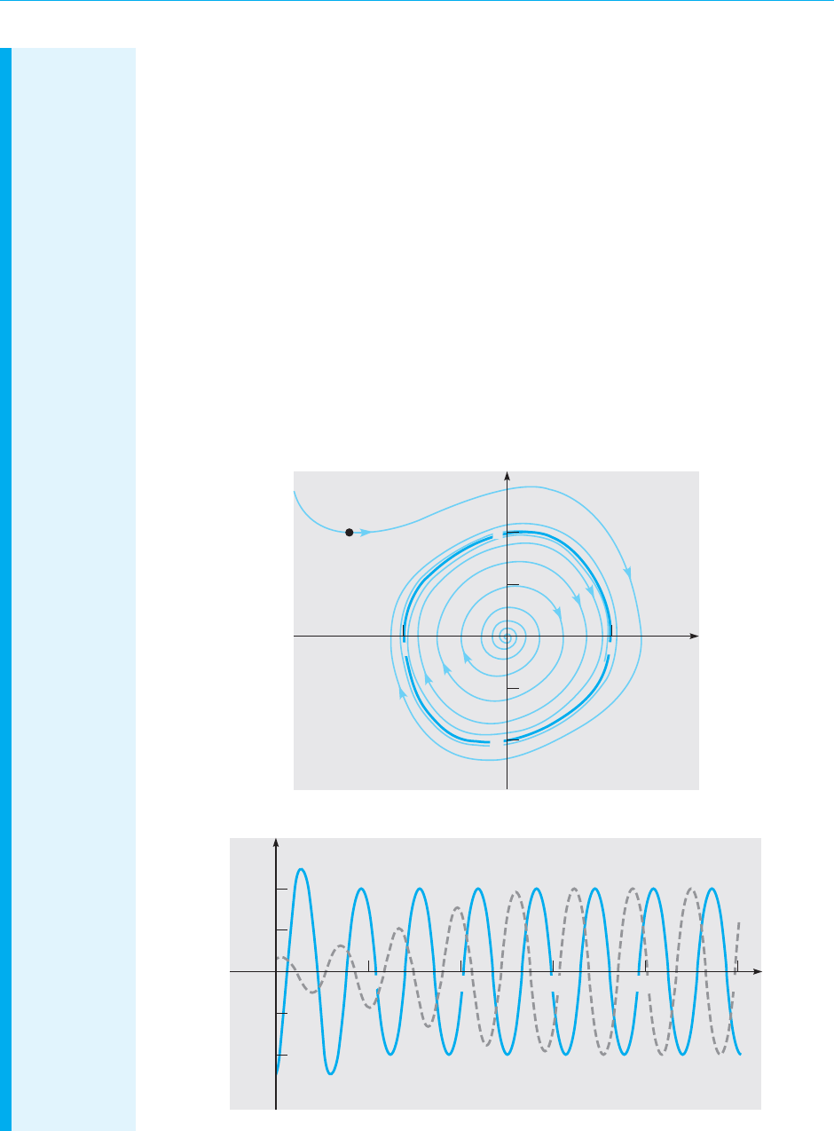
August 7, 2012 21:05 c09 Sheet number 77 Page number 571 cyan black
9.7 Periodic Solutions and Limit Cycles 571
It is possible to show, by a more intricate analysis, that the van der Pol equation does have a
unique limit cycle. However, we will not follow this line of argument further. We turn instead
to a different approach in which we plot numerically computed approximations to solutions.
Experimental observations indicate that the van der Pol equation has an asymptotically stable
periodic solution whose period and amplitude depend on the parameter µ. By looking at
graphs of trajectories in the phase plane and of u versus t, we can gain some understanding of
this periodic behavior.
Figure 9.7.2 shows two trajectories of the van der Pol equation in the phase plane for
µ = 0.2. The trajectory starting near the origin spirals outward in the clockwise direction;
this is consistent with the behavior of the linear approximation near the origin. The other
trajectory passes through (−3, 2) and spirals inward, again in the clockwise direction.
Both trajectories approach a closed curve that corresponds to a stable periodic solution. In
Figure 9.7.3 we show the plots of u versus t for the solutions corresponding to the trajectories
in Figure 9.7.2. The solution that is initially smaller gradually increases in amplitude, while
the larger solution gradually decays. Both solutions approach a stable periodic motion that
corresponds to the limit cycle. Figure 9.7.3 also shows that there is a phase difference between
the two solutions as they approach the limit cycle. The plots of u versus t are nearly sinusoidal
in shape, consistent with the nearly circular limit cycle in this case.
x
y
–2
–1
1
2
–2
2
(–3, 2)
FIGURE 9.7.2 Trajectories of the van der Pol equation (17) for µ = 0.2.
u
t
1
2
–1
–2
10 20 30 40 50
FIGURE 9.7.3 Plots of u versus t for the trajectories in Figure 9.7.2.

August 7, 2012 21:05 c09 Sheet number 78 Page number 572 cyan black
572 Chapter 9. Nonlinear Differential Equations and Stability
Figures 9.7.4 and 9.7.5 show similar plots for the case µ = 1. Trajectories again move clock-
wise in the phase plane, but the limit cycle is considerably different from a circle. The plots
of u versus t tend more rapidly to the limiting oscillation, and again show a phase difference.
The oscillations are somewhat less symmetric in this case, rising somewhat more steeply than
they fall.
y
x
1–1
2
1
–1
–2
2–2
FIGURE 9.7.4 Trajectories of the van der Pol equation (17) for µ = 1.
2
1
–1
–2
u
t
10 20 30 40 50
FIGURE 9.7.5 Plots of u versus t for the trajectories in Figure 9.7.4.
Figure 9.7.6 shows the phase plane for µ = 5. The motion remains clockwise, and the limit
cycle is even more elongated, especially in the y direction. Figure 9.7.7 is a plot of u versus t.
Although the solution starts far from the limit cycle, the limiting oscillation is virtually reached
in a fraction of a period. Starting from one of its extreme values on the x-axis in the phase
plane, the solution moves toward the other extreme position slowly at first, but once a certain
point on the trajectory is reached, the remainder of the transition is completed very swiftly.
The process is then repeated in the opposite direction. The waveform of the limit cycle, as
shown in Figure 9.7.7, is quite different from a sine wave.

August 7, 2012 21:05 c09 Sheet number 79 Page number 573 cyan black
9.7 Periodic Solutions and Limit Cycles 573
y
t
10
5
2
–5
–10
–2
FIGURE 9.7.6 Trajectories of the van der Pol equation (17) for µ = 5.
2
1
–1
–2
u
t
10 20 30 40 50
FIGURE 9.7.7 Plot of u versus t for the outward spiralling trajectory in Figure 9.7.6.
These graphs clearly show that in the absence of external excitation, the van der Pol
oscillator has a certain characteristic mode of vibration for each value of µ. The graphs of
u versus t show that the amplitude of this oscillation changes very little with µ, but the period
increases as µ increases. At the same time, the waveform changes from one that is very nearly
sinusoidal to one that is much less smooth.
The presence of a single periodic motion that attracts all (nearby) solutions—that is, an
asymptotically stable limit cycle—is one of the characteristic phenomena associated with
nonlinear differential equations.

August 7, 2012 21:05 c09 Sheet number 80 Page number 574 cyan black
574 Chapter 9. Nonlinear Differential Equations and Stability
PROBLEMS In each of Problems 1 through 6, an autonomous system is expressed in polar coordinates.
Determine all periodic solutions, all limit cycles, and the stability characteristics of all peri-
odic solutions.
1. dr/dt = r
2
(1 − r
2
), dθ/dt = 12.dr/dt = r(1 − r)
2
, dθ/dt =−1
3. dr/dt = r(r − 1)(r − 3), dθ/dt = 14.dr/dt = r(1 − r)(r − 2), dθ/dt =−1
5. dr/dt = sin πr, dθ/dt = 1
6. dr/dt = r|r − 2|(r − 3), dθ/dt =−1
7. If x = r cos θ, y = r sin θ, show that y(dx/dt) − x(dy/dt) =−r
2
(dθ/dt).
8. (a) Show that the system
dx/dt =−y + xf (r)/r, dy/dt = x + yf (r)/r
has periodic solutions corresponding to the zeros of f (r). What is the direction of motion
on the closed trajectories in the phase plane?
(b) Let f (r) = r(r − 2)
2
(r
2
− 4r + 3). Determine all periodic solutions, and determine
their stability characteristics.
9. Determine the periodic solutions, if any, of the system
dx
dt
= y +
x
!
x
2
+ y
2
(x
2
+ y
2
− 2),
dy
dt
=−x +
y
!
x
2
+ y
2
(x
2
+ y
2
− 2).
10. Using Theorem 9.7.2, show that the linear autonomous system
dx/dt = a
11
x + a
12
y, dy/dt = a
21
x + a
22
y
does not have a periodic solution (other than x = 0, y = 0) if a
11
+ a
22
̸= 0.
In each of Problems 11 and 12, show that the given system has no periodic solutions other than
constant solutions.
11. dx/dt = x + y + x
3
− y
2
, dy/dt =−x + 2y + x
2
y + y
3
/3
12. dx/dt =−2x − 3y − xy
2
, dy/dt = y + x
3
− x
2
y
13. Prove Theorem 9.7.2 by completing the following argument. According to Green’s the-
orem in the plane, if C is a sufficiently smooth simple closed curve, and if F and G are
continuous and have continuous first partial derivatives, then
"
C
.
F(x, y) dy − G(x, y) dx
/
=
""
R
.
F
x
(x, y) + G
y
(x, y)
/
dA,
where C is traversed counterclockwise and R is the region enclosed by C. Assume that
x = φ(t), y = ψ(t) is a solution of the system (15) that is periodic with period T. Let C be
the closed curve given by x = φ(t), y = ψ(t) for 0 ≤ t ≤ T. Show that for this curve, the
line integral is zero. Then show that the conclusion of Theorem 9.7.2 must follow.
14.
(a) By examining the graphs of u versus t in Figures 9.7.3, 9.7.5, and 9.7.7, estimate the
period T of the van der Pol oscillator in these cases.
(b) Calculate and plot the graphs of solutions of the van der Pol equation for other values
of the parameter µ. Estimate the period T in these cases also.
(c) Plot the estimated values of T versus µ. Describe how T depends on µ.

August 7, 2012 21:05 c09 Sheet number 81 Page number 575 cyan black
9.7 Periodic Solutions and Limit Cycles 575
15. The equation
u
′′
− µ(1 −
1
3
u
′2
)u
′
+ u = 0
is often called the Rayleigh
13
equation.
(a) Write the Rayleigh equation as a system of two first order equations.
(b) Show that the origin is the only critical point of this system. Determine its type and
whether it is asymptotically stable, stable, or unstable.
(c) Let µ = 1. Choose initial conditions, and compute the corresponding solution of
the system on an interval such as 0 ≤ t ≤ 20 or longer. Plot u versus t, and also plot the
trajectory in the phase plane. Observe that the trajectory approaches a closed curve (limit
cycle). Estimate the amplitude A and the period T of the limit cycle.
(d) Repeat part (c) for other values of µ, such as µ = 0.2, 0.5, 2, and 5. In each case
estimate the amplitude A and the period T.
(e) Describe how the limit cycle changes as µ increases. For example, make a table of
values and/or plot A and T as functions of µ.
16. Consider the system of equations
x
′
= µx + y − x(x
2
+ y
2
), y
′
=−x + µy − y(x
2
+ y
2
), (i)
where µ is a parameter. Observe that this system is the same as the one in Example 1,
except for the introduction of µ.
(a) Show that the origin is the only critical point.
(b) Find the linear system that approximates Eqs. (i) near the origin, and find its eigen-
values. Determine the type and stability of the critical point at the origin. How does this
classification depend on µ?
(c) Referring to Example 1 if necessary, rewrite Eqs. (i) in polar coordinates.
(d) Show that when µ>0, there is a periodic solution r =
√
µ. By solving the system
found in part (c), or by plotting numerically computed approximate solutions, conclude
that this periodic solution attracts all other nonzero solutions.
Note: As the parameter µ increases through the value zero, the previously asymptot-
ically stable critical point at the origin loses its stability, and simultaneously a new
asymptotically stable solution (the limit cycle) emerges. Thus the point µ = 0isa
bifurcation point; this type of bifurcation is called a Hopf
14
bifurcation.
17.
Consider the van der Pol system
x
′
= y, y
′
=−x + µ(1 − x
2
)y,
where now we allow the parameter µ to be any real number.
(a) Show that the origin is the only critical point. Determine its type, its stability property,
and how these depend on µ.
13
John William Strutt (1842–1919), the third Lord Rayleigh, made notable contributions in several areas
of mathematical physics. His theory of scattering (1871) provided the first correct explanation of why
the sky is blue, and his two volume treatise The Theory of Sound, published in 1877 and 1878,is one of the
classics of applied mathematics. Apart from five years as Cavendish Professor of Physics at Cambridge,
he worked primarily in his private laboratory at home. He was awarded the Nobel Prize for Physics in
1904 for the discovery of argon.
14
Eberhard Hopf (1902–1983) was born in Austria and educated at the University of Berlin but spent
much of his life in the United States, mainly at Indiana University. He was one of the founders of ergodic
theory. Hopf bifurcations are named for him in honor of his rigorous treatment of them in a 1942 paper.

August 7, 2012 21:05 c09 Sheet number 82 Page number 576 cyan black
576 Chapter 9. Nonlinear Differential Equations and Stability
(b) Let µ =−1; draw a phase portrait, and conclude that there is a periodic solution that
surrounds the origin. Observe that this periodic solution is unstable. Compare your plot
with Figure 9.7.4.
(c) Draw a phase portrait for a few other negative values of µ. Describe how the shape
of the periodic solution changes with µ.
(d) Consider small positive or negative values of µ. By drawing phase portraits,determine
how the periodic solution changes as µ → 0. Compare the behavior of the van der Pol
system as µ increases through zero with the behavior of the system in Problem 16.
Problems 18 and 19 extend the consideration of the Rosenzweig–MacArthur predator–
prey model introduced in Problem 13 of Section 9.5.
18.
Consider the system
x
′
= x
'
2.4 − 0.2x −
2y
x + 6
(
, y
′
= y
'
−0.25 +
x
x + 6
(
.
Observe that this system differs from that in Problem 13 of Section 9.5 only in the growth
rate for the prey.
(a) Find all of the critical points.
(b) Determine the type and stability of each critical point.
(c) Draw a phase portrait in the first quadrant,and conclude that there is an asymptotically
stable limit cycle. Thus this model predicts a stable long-term oscillation of the prey and
predator populations.
19.
Consider the system
x
′
= x
'
a − 0.2x −
2y
x + 6
(
, y
′
= y
'
−0.25 +
x
x + 6
(
,
where a is a positive parameter. Observe that this system includes the one in Problem 18
above and also the one in Problem 13 in Section 9.5.
(a) Find all of the critical points.
(b) Consider the critical point in the interior of the first quadrant. Find the eigenvalues of
the approximate linear system. Determine the value a
0
where this critical point changes
from asymptotically stable to unstable.
(c) Draw a phase portrait for a value of a slightly greater than a
0
. Observe that a limit
cycle has appeared. How does the limit cycle change as a increases further?
20.
There are certain chemical reactions in which the constituent concentrations oscillate
periodically over time. The system
x
′
= 1 − (b + 1)x + x
2
y/4, y
′
= bx − x
2
y/4
is a special case of a model, known as the Brusselator, of this kind of reaction. Assume
that b is a positive parameter, and consider solutions in the first quadrant of the xy-plane.
(a) Show that the only critical point is (1, 4b).
(b) Find the eigenvalues of the approximate linear system at the critical point.
(c) Classify the critical point as to type and stability. How does the classification depend
on b?
(d) As b increases through a certain value b
0
, the critical point changes from asymptoti-
cally stable to unstable. What is that value b
0
?

August 7, 2012 21:05 c09 Sheet number 83 Page number 577 cyan black
9.8 Chaos and Strange Attractors: The Lorenz Equations 577
(e) Plot trajectories in the phase plane for values of b slightly less than and slightly greater
than b
0
. Observe the limit cycle when b > b
0
; the Brusselator has a Hopf bifurcation point
at b
0
.
(f) Plot trajectories for several values of b > b
0
and observe how the limit cycle deforms
as b increases.
21.
The system
x
′
= 3(x + y −
1
3
x
3
− k), y
′
=−
1
3
(x + 0.8y − 0.7)
is a special case of the Fitzhugh–Nagumo
15
equations, which model the transmission of
neural impulses along an axon. The parameter k is the external stimulus.
(a) Show that the system has one critical point regardless of the value of k.
(b) Find the critical point for k = 0, and show that it is an asymptotically stable spiral
point. Repeat the analysis for k = 0.5, and show that the critical point is now an unstable
spiral point. Draw a phase portrait for the system in each case.
(c) Find the value k
0
where the critical point changes from asymptotically stable to
unstable. Find the critical point and draw a phase portrait for the system for k = k
0
.
(d) For k > k
0
the system exhibits an asymptotically stable limit cycle; the system has a
Hopf bifurcation point at k
0
. Draw a phase portrait for k = 0.4, 0.5, and 0.6; observe that
the limit cycle is not small when k is near k
0
. Also plot x versus t and estimate the period
T in each case.
(e) As k increases further, there is a value k
1
at which the critical point again becomes
asymptotically stable and the limit cycle vanishes. Find k
1
.
9.8 Chaos and Strange Attractors: The Lorenz Equations
In principle,the methods described in this chapter for second order autonomous sys-
tems can be applied to higher order systems as well. In practice, several difficulties
arise when we try to do this. One problem is that there is simply a greater num-
ber of possible cases that can occur, and the number increases with the number of
equations in the system (and the dimension of the phase space). Another problem is
the difficulty of graphing trajectories accurately in a phase space of more than two
dimensions; even in three dimensions it may not be easy to construct a clear and
understandable plot of the trajectories, and it becomes more difficult as the number
of variables increases. Finally—and this has been widely recognized only since the
1970s—there are different and very complex phenomena that can occur, and fre-
quently do occur, in systems of third and higher order that are not present in second
order systems. Our goal in this section is to provide a brief introduction to some of
these phenomena by discussing one particular three-dimensional autonomous sys-
tem that has been intensively studied. In some respects, the presentation here is
similar to the treatment of the logistic difference equation in Section 2.9.
15
Richard Fitzhugh (1922–2007) of the United States Public Health Service and Jin-Ichi Nagumo (1926–
1999) of the University of Tokyo independently proposed a simplification of the Hodgkin–Huxley model
of neural transmission around 1961.

August 7, 2012 21:05 c09 Sheet number 84 Page number 578 cyan black
578 Chapter 9. Nonlinear Differential Equations and Stability
An important problem in meteorology, and in other applications of fluid dynam-
ics, concerns the motion of a layer of fluid, such as the earth’s atmosphere, that is
warmer at the bottom than at the top; see Figure 9.8.1. If the vertical temperature
difference 5T is small, then there is a linear variation of temperature with altitude
but no significant motion of the fluid layer. However, if 5T is large enough, then the
warmer air rises, displacing the cooler air above it, and a steady convective motion
results. If the temperature difference increases further, then eventually the steady
convective flow breaks up and a more complex and turbulent motion ensues.
Cooler
Warmer
Temperature
difference ∆
T
FIGURE 9.8.1 A layer of fluid heated from below.
While investigating this phenomenon, Edward N. Lorenz
16
was led (by a pro-
cess too involved to describe here) to the nonlinear autonomous three-dimensional
system
dx/dt = σ(−x + y),
dy/dt = rx − y − xz, (1)
dz/dt =−bz + xy.
Equations (1) are now commonly referred to as the Lorenz equations.
17
Observe that
the second and third equations involve quadratic nonlinearities. However,except for
being a system of three equations, superficially the Lorenz equations appear no more
complicated than the competing species and predator–prey equations discussed in
Sections 9.4 and 9.5. The variable x in Eqs. (1) is related to the intensity of the
fluid motion, while the variables y and z are related to the temperature variations
in the horizontal and vertical directions. The Lorenz equations also involve three
parameters σ, r, and b, all of which are real and positive. The parameters σ and b
depend on the material and geometrical properties of the fluid layer. For the earth’s
atmosphere, reasonable values of these parameters are σ = 10 and b = 8/3; they
will be assigned these values in much of what follows in this section. The parameter r,
on the other hand,is proportional to the temperature difference 5T,and our purpose
is to investigate how the nature of the solutions of Eqs. (1) changes with r.
16
Edward N. Lorenz (1917–2008), an American meteorologist, received his Ph.D. from the Massachusetts
Institute of Technology in 1948 and was associated with that institution throughout his scientific career.
His first studies of the system (1) appeared in a famous 1963 paper (cited in the references) dealing with
the stability of fluid flows in the atmosphere.
17
A very thorough treatment of the Lorenz equations appears in the book by Sparrow listed in the
references at the end of this chapter.

August 7, 2012 21:05 c09 Sheet number 85 Page number 579 cyan black
9.8 Chaos and Strange Attractors: The Lorenz Equations 579
Before proceeding further, we note that for an autonomous system of three first
order equations
dx/dt = F(x, y, z), dy/dt = G(x, y, z), dz/dt = H(x, y, z), (2)
the Jacobian matrix J is defined by
J =
⎛
⎜
⎝
F
x
F
y
F
z
G
x
G
y
G
z
H
x
H
y
H
z
⎞
⎟
⎠
. (3)
Thus, for the Lorenz equations (1), the Jacobian matrix is
J =
⎛
⎜
⎝
−σσ0
r − z −1 −x
yx−b
⎞
⎟
⎠
. (4)
The first step in analyzing the Lorenz equations is to locate the critical points by
solving the algebraic system
σx − σy = 0,
rx − y − xz = 0, (5)
−bz + xy = 0.
From the first equation we have y = x. Then, eliminating y from the second and
third equations, we obtain
x(r − 1 − z) = 0, (6)
−bz + x
2
= 0. (7)
One way to satisfy Eq. (6) is to choose x = 0. Then it follows that y = 0 and,
from Eq. (7), z = 0. Alternatively, we can satisfy Eq. (6) by choosing z = r − 1. Then
Eq. (7) requires that x =±
√
b(r − 1) and then y =±
√
b(r − 1) also. Observe that
these expressions for x and y are real only when r ≥ 1. Thus (0, 0, 0), which we will
denote by P
1
, is a critical point for all values of r, and it is the only critical point
for r < 1. However, when r > 1, there are also two other critical points, namely,
(
√
b(r − 1),
√
b(r − 1), r − 1) and (−
√
b(r − 1), −
√
b(r − 1), r − 1). We will denote
the latter two points by P
2
and P
3
, respectively. Note that all three critical points
coincide when r = 1. As r increases through the value 1, the critical point P
1
at the
origin bifurcates, and the critical points P
2
and P
3
come into existence.
Next we will determine the local behavior of solutions in the neighborhood of
each critical point. Although much of the following analysis can be carried out for
arbitrary values of σ and b, we will simplify our work by using the values σ = 10 and
b = 8/3. Near the origin (the critical point P
1
), the approximating linear system is
⎛
⎜
⎝
x
y
z
⎞
⎟
⎠
′
=
⎛
⎜
⎝
−10 10 0
r −10
00−8/3
⎞
⎟
⎠
⎛
⎜
⎝
x
y
z
⎞
⎟
⎠
. (8)

August 7, 2012 21:05 c09 Sheet number 86 Page number 580 cyan black
580 Chapter 9. Nonlinear Differential Equations and Stability
The eigenvalues
18
are determined from the equation
3
3
3
3
3
3
3
−10 − λ 10 0
r −1 − λ 0
00−8/3 − λ
3
3
3
3
3
3
3
=−(8/3 + λ)[λ
2
+ 11λ − 10(r − 1)]=0. (9)
Therefore,
λ
1
=−
8
3
, λ
2
=
−11 −
√
81 + 40r
2
, λ
3
=
−11 +
√
81 + 40r
2
. (10)
Note that all three eigenvalues are negative for r < 1; for example, when r = 1/2,
the eigenvalues are λ
1
=−8/3, λ
2
=−10.52494, λ
3
=−0.47506. Hence the origin is
asymptotically stable for this range of r both for the linear approximation (8) and
for the original system (1). However, λ
3
changes sign when r = 1 and is positive for
r > 1. The value r = 1 corresponds to the initiation of convective flow in the physical
problem described earlier. The origin is unstable for r > 1; all solutions starting near
the origin tend to grow, except for those lying precisely in the plane determined
by the eigenvectors associated with λ
1
and λ
2
[or, for the nonlinear system (1), in a
certain surface tangent to this plane at the origin].
The second critical point is P
2
(
!
8(r − 1)/3,
!
8(r − 1)/3, r − 1) for r > 1. To con-
sider the neighborhood of this critical point, let u, v, and w be the perturbations from
the critical point in the x-, y-, and z-directions, respectively.The approximating linear
system is
⎛
⎜
⎝
u
v
w
⎞
⎟
⎠
′
=
⎛
⎜
⎝
−10 10 0
1 −1 −
!
8(r − 1)/3
!
8(r − 1)/3
!
8(r − 1)/3 −8/3
⎞
⎟
⎠
⎛
⎜
⎝
u
v
w
⎞
⎟
⎠
. (11)
The eigenvalues of the coefficient matrix of Eq. (11) are determined from the
equation
3λ
3
+ 41λ
2
+ 8(r + 10)λ + 160(r − 1) = 0, (12)
which is obtained by straightforward algebraic steps that are omitted here. The
solutions of Eq. (12) depend on r in the following way:
For 1 < r < r
1
∼
=
1.3456 there are three negative real eigenvalues.
For r
1
< r < r
2
∼
=
24.737 there areone negative realeigenvalue and two complex
eigenvalues with negative real part.
For r
2
< r there are one negative real eigenvalue and two complex eigenvalues
with positive real part.
The same results are obtained for the critical point P
3
. Thus there are several
different situations.
For 0 < r < 1 the only critical point is P
1
and it is asymptotically stable. All
solutions approach this point (the origin) as t →∞.
18
Since r appears as a parameter in the Lorenz equations, we will use λ to denote the eigenvalues.

August 7, 2012 21:05 c09 Sheet number 87 Page number 581 cyan black
9.8 Chaos and Strange Attractors: The Lorenz Equations 581
For 1 < r < r
1
the critical points P
2
and P
3
are asymptotically stable and P
1
is
unstable. All nearby solutions approach one or the other of the points P
2
and P
3
exponentially.
For r
1
< r < r
2
the critical points P
2
and P
3
are asymptotically stable and P
1
is
unstable. All nearby solutions approach one or the other of the points P
2
and P
3
;
most of them spiral inward to the critical point.
For r
2
< r all three critical points are unstable. Most solutions near P
2
or P
3
spiral
away from the critical point.
However, this is by no means the end of the story. Let us consider solutions for r
somewhat greater than r
2
. In this case P
1
has one positive eigenvalue, and each of
P
2
and P
3
has a pair of complex eigenvalues with positive real part. A trajectory can
approach any one of the critical points only on certain highly restricted paths. The
slightest deviation from these paths causes the trajectory to depart from the critical
point. Since none of thecritical pointsis stable,one might expect thatmost trajectories
would approach infinity for large t. However,it can be shown that all solutions remain
bounded ast →∞;see Problem 5. In fact,it canbe shown that all solutions ultimately
approach a certain limiting set of points that has zero volume. Indeed, this is true not
only for r > r
2
but for all positive values of r.
A plot of computed values of x versus t for a typical solution with r > r
2
is shown
in Figure 9.8.2. Note that the solution oscillates back and forth between positive and
negative values in a rather erratic manner. Indeed, the graph of x versus t resem-
bles a random vibration, although the Lorenz equations are entirely deterministic
and the solution is completely determined by the initial conditions. Nevertheless,
the solution also exhibits a certain regularity in that the frequency and amplitude
of the oscillations are essentially constant in time.
16
8
–8
–16
x
t
10 20
FIGURE 9.8.2 A plot of x versus t for the Lorenz equations (1) with r = 28;
the initial point is (5, 5, 5).
The solutions of the Lorenz equations are also extremely sensitive to perturbations
in the initial conditions. Figure 9.8.3 shows the graphs of computed values of x versus
t for the two solutions whose initial points are (5, 5, 5) and (5.01, 5, 5). The dashed
graph is the same as the one in Figure 9.8.2, while the solid graph starts at a nearby
point. The two solutions remain close until t is near 10, after which they are quite
different and, indeed, seem to have no relation to each other. It was this property
that particularly attracted the attention of Lorenz in his original study of these

August 7, 2012 21:05 c09 Sheet number 88 Page number 582 cyan black
582 Chapter 9. Nonlinear Differential Equations and Stability
16
8
–8
10 20
–16
x
t
FIGURE 9.8.3 Plots of x versus t for two initially nearby solutions of Lorenz equations with
r = 28; the initial point is (5, 5, 5) for the dashed curve and is (5.01, 5, 5) for the solid curve.
equations, and it caused him to conclude that accurate detailed long-range weather
predictions are probably not possible.
The attracting set in this case, although of zero volume, has a rather complicated
structure and is called a strange attractor. The term chaotic has come into general
use to describe solutions such as those shown in Figures 9.8.2 and 9.8.3.
To determine how and when the strange attractor is created, it is illuminating to
investigate solutions for smaller values of r.Forr = 21,solutions starting at three dif-
ferent initial points are shown in Figure 9.8.4. For the initial point (3, 8, 0) the solution
begins to converge to the point P
3
almost at once; see Figure 9.8.4a. For the second
initial point (5, 5, 5) there is a fairly short interval of transient behavior, after which
the solution converges to P
2
; see Figure 9.8.4b. However, as shown in Figure 9.8.4c,
for the third initial point (5, 5, 10) there is a much longer interval of transient chaotic
behavior before the solution eventually converges to P
2
.Asr increases, the duration
of the chaotic transient behavior also increases. When r = r
3
∼
=
24.06, the chaotic
transients appear to continue indefinitely,and the strange attractor comes into being.
We can also show the trajectories of the Lorenz equations in the three-
dimensional phase space, or at least projections of them in various planes. Figures
9.8.5 and 9.8.6 show projections in the xy- and xz-planes, respectively, of the tra-
jectory starting at (5, 5, 5). Observe that the graphs in these figures appear to cross
over themselves repeatedly, but this cannot be true for the actual trajectories in
three-dimensional space because of the general uniqueness theorem. The apparent
crossings are due wholly to the two-dimensional character of the figures.
The sensitivity of solutions to perturbations of the initial data also has impli-
cations for numerical computations, such as those reported here. Different step
sizes, different numerical algorithms, and even the execution of the same algorithm
on different machines will introduce small differences in the computed solution,
which eventually lead to large deviations. For example, the exact sequence of pos-
itive and negative loops in the calculated solution depends strongly on the precise
numerical algorithm and its implementation, as well as on the initial conditions.
However, the general appearance of the solution and the structure of the attracting
set are independent of all these factors.

August 7, 2012 21:05 c09 Sheet number 89 Page number 583 cyan black
9.8 Chaos and Strange Attractors: The Lorenz Equations 583
16
8
–8
–16
12 24
(a)
x
t
12 24
(b)
16
8
–8
–16
x
t
6321
48
60 72
(c)
16
8
–8
–16
x
t
24
FIGURE 9.8.4 Plots of x versus t for three solutions of Lorenz equations with r = 21.
(a) Initial point is (3, 8, 0). (b) Initial point is (5, 5, 5). (c) Initial point is (5, 5, 10).
x
y
20
10
–20
–10
–20
20
FIGURE 9.8.5 Projections of a trajectory of the Lorenz equations
(with r = 28) in the xy-plane.

August 7, 2012 21:05 c09 Sheet number 90 Page number 584 cyan black
584 Chapter 9. Nonlinear Differential Equations and Stability
x
z
10
40
30
–10 10
FIGURE 9.8.6 Projections of a trajectory of the Lorenz equations
(with r = 28) in the xz-plane.
Solutions of the Lorenz equations for other parameter ranges exhibit other
interesting types of behavior. For example, for certain values of r greater than
r
2
, intermittent bursts of chaotic behavior separate long intervals of apparently
steady periodic oscillation. For other ranges of r,solutions show the period-doubling
property that we saw in Section 2.9 for the logistic difference equation. Some of these
features are taken up in the problems.
Since about 1975 the Lorenz equations and other higher-dimensional autonomous
systems have been studied intensively, and this is one of the most active areas of cur-
rent mathematical research. Chaotic behavior of solutions appears to be much more
common than was suspected at first, and many questions remain unanswered. Some
of these are mathematical in nature, while others relate to the physical applications
or interpretations of solutions.
PROBLEMS Problems 1 through 3 ask you to fill in some of the details of the analysis of the Lorenz equations
in this section.
1. (a) Show that the eigenvalues of the linear system (8), valid near the origin, are given by
Eq. (10).
(b) Determine the corresponding eigenvectors.
(c) Determine the eigenvalues and eigenvectors of the system (8) in the case where r = 28.
2.
(a) Show that the linear approximation valid near the critical point P
2
is given by Eq. (11).
(b) Show that the eigenvalues of the system (11) satisfy Eq. (12).
(c) For r = 28, solve Eq. (12) and thereby determine the eigenvalues of the system (11).
3.
(a) By solving Eq. (12) numerically, show that the real part of the complex roots changes
sign when r
∼
=
24.737.
(b) Show that a cubic polynomial x
3
+ Ax
2
+ Bx + C has one real zero and two pure
imaginary zeros only if AB = C.
(c) By applying the result of part (b) to Eq. (12), show that the real part of the complex
roots changes sign when r = 470/19.
4. Use the Liapunov function V(x, y, z) = x
2
+ σy
2
+ σz
2
to show that the origin is a globally
asymptotically stable critical point for the Lorenz equations (1) if r < 1.

August 7, 2012 21:05 c09 Sheet number 91 Page number 585 cyan black
9.8 Chaos and Strange Attractors: The Lorenz Equations 585
5. Consider the ellipsoid
V(x, y, z) = rx
2
+ σy
2
+ σ(z − 2r)
2
= c > 0.
(a) Calculate dV/dt along trajectories of the Lorenz equations (1).
(b) Determine a sufficient condition on c so that every trajectory crossing V(x, y, z) = c
is directed inward.
(c) Evaluate the condition found in part (b) for the case σ = 10, b = 8/3, r = 28.
Problems 6 through 10 suggest some further investigations of the Lorenz equations.
6.
For r = 28, plot x versus t for the cases shown in Figures 9.8.2 and 9.8.3. Do your graphs
agree with those shown in the figures? Recall the discussion of numerical computation in
the text.
7.
For r = 28, plot the projections in the xy- and xz-planes, respectively, of the trajectory
starting at the point (5, 5, 5). Do the graphs agree with those in Figures 9.8.5 and 9.8.6?
8.
(a) For r = 21,plot x versus t for the solutions starting at the initial points (3, 8, 0),(5, 5,5),
and (5, 5,10). Use a t-interval of at least 0 ≤ t ≤ 30. Compare your graphs with those in
Figure 9.8.4.
(b) Repeat the calculation in part (a) for r = 22,r = 23, and r = 24. Increase the t interval
as necessary so that you can determine when each solution begins to converge to one of
the critical points. Record the approximate duration of the chaotic transient in each case.
Describe how this quantity depends on the value of r.
(c) Repeat the calculations in parts (a) and (b) for values of r slightly greater than 24.
Try to estimate the value of r for which the duration of the chaotic transient approaches
infinity.
9.
For certain r intervals, or windows, the Lorenz equations exhibit a period-doubling prop-
erty similar to that of the logistic difference equation discussed in Section 2.9. Careful
calculations may reveal this phenomenon.
(a) One period-doubling window contains the value r = 100. Let r = 100 and plot the
trajectory starting at (5, 5, 5) or some other initial point of your choice. Does the solution
appear to be periodic? What is the period?
(b) Repeat the calculation in part (a) for slightly smaller values of r. When r
∼
=
99.98, you
may be able to observe that the period of the solution doubles. Try to observe this result
by performing calculations with nearby values of r.
(c) As r decreases further, the period of the solution doubles repeatedly. The next period
doubling occurs at about r = 99.629. Try to observe this by plotting trajectories for nearby
values of r.
10.
Now consider values of r slightly larger than those in Problem 9.
(a) Plot trajectories of the Lorenz equations for values of r between 100 and 100.78. You
should observe a steady periodic solution for this range of r values.
(b) Plot trajectories for values of r between 100.78 and 100.8. Determine as best you can
how and when the periodic trajectory breaks up.
The Rössler
19
System. The system
x
′
=−y − z, y
′
= x + ay, z
′
= b + z(x − c), (i)
19
Otto E. Rössler (1940– ), a German medical doctor and biochemist, was a student and later became
a faculty member at the University of Tübingen. The equations named for him first appeared in a paper
he published in 1976.

August 7, 2012 21:05 c09 Sheet number 92 Page number 586 cyan black
586 Chapter 9. Nonlinear Differential Equations and Stability
where a, b, and c are positive parameters, is known as the Rössler system.
20
It is a relatively
simple system, consisting of two linear equations and a third equation with a single quadratic
nonlinearity. In Problems 11 through 15, we ask you to carry out some numerical investigations
of this system, with the goal of exploring its period-doubling property. To simplify matters, set
a = 0.25, set b = 0.5, and let c > 0 remain arbitrary.
11.
(a) Show that there are no critical points when c <
√
0.5, there is one critical point for
c =
√
0.5, and there are two critical points when c >
√
0.5.
(b) Find the critical point(s) and determine the eigenvalues of the associated Jacobian
matrix when c =
√
0.5 and when c = 1.
(c) How do you think trajectories of the system will behave for c = 1? Plot the trajectory
starting at the origin. Does it behave the way that you expected?
(d) Choose one or two other initial points, and plot the corresponding trajectories. Do
these plots agree with your expectations?
12.
(a) Let c = 1.3. Find the critical points and the corresponding eigenvalues. What
conclusions, if any, can you draw from this information?
(b) Plot the trajectory starting at the origin. What is the limiting behavior of this trajec-
tory? To see the limiting behavior clearly, you may wish to choose a t-interval for your
plot so that the initial transients are eliminated.
(c) Choose one or two other initial points, and plot the corresponding trajectories. Are
the limiting behavior(s) the same as in part (b)?
(d) Observe that there is a limit cycle whose basin of attraction is fairly large (although
not all of xyz-space). Draw a plot of x, y,orz versus t,and estimate the period T
1
of motion
around the limit cycle.
13.
The limit cycle found in Problem 12 comes into existence as a result of a Hopf bifurcation
at a value c
1
of c between 1 and 1.3. Determine, or at least estimate more precisely, the
value of c
1
. There are several ways in which you might do this.
(a) Draw plots of trajectories for different values of c.
(b) Calculate eigenvalues at critical points for different values of c .
(c) Use the result of Problem 3(b) above.
14.
(a) Let c = 3. Find the critical points and the corresponding eigenvalues.
(b) Plot the trajectory starting at the point (1, 0, −2). Observe that the limit cycle now
consists of two loops before it closes; it is often called a 2-cycle.
(c) Plot x, y,orz versus t, and show that the period T
2
of motion on the 2-cycle is very
nearly double the period T
1
of the simple limit cycle in Problem 12. There has been a
period-doubling bifurcation of cycles for a certain value of c between 1.3 and 3.
15.
(a) Let c = 3.8. Find the critical points and the corresponding eigenvalues.
(b) Plot the trajectory starting at the point (1, 0, −2). Observe that the limit cycle is now a
4-cycle. Find the period T
4
of motion. Another period-doubling bifurcation has occurred
for c between 3 and 3.8.
(c) For c = 3.85, show that the limit cycle is an 8-cycle. Verify that its period is very close
to eight times the period of the simple limit cycle in Problem 12.
Note: As c increases further, there is an accelerating cascade of period-doubling bifurca-
tions. The bifurcation values of c converge to a limit, which marks the onset of chaos.
20
See the book by Strogatz for a more extensive discussion and further references.

August 7, 2012 21:05 c09 Sheet number 93 Page number 587 cyan black
References 587
REFERENCES There are many books that expand on the material treated in this chapter. They include
Drazin, P. G., Nonlinear Systems (Cambridge: Cambridge University Press, 1992).
Glendinning, P., Stability, Instability, and Chaos (Cambridge: Cambridge University Press, 1994).
Grimshaw, R., Nonlinear Ordinary Differential Equations (Oxford:Blackwell Scientific Publications, 1990;
New York: CRC Press, 1991).
Hirsch, M. W., Smale, S., and Devaney, R. L., Differential Equations, Dynamical Systems, and an Introduc-
tion to Chaos (2nd edition) (San Diego, CA:Academic Press, 2004).
Hubbard, J. H., and West, B. H., Differential Equations: A Dynamical Systems Approach, Higher Dimen-
sional Systems (New York/Berlin: Springer-Verlag, 1995)
Two books that are especially notable from the point of view of applications are
Danby, J. M. A., Computer Applications to Differential Equations (Englewood Cliffs, NJ: Prentice-Hall,
1985).
Strogatz, S. H., Nonlinear Dynamics and Chaos (Reading, MA: Addison-Wesley, 1994).
A good reference on Liapunov’s second method is
LaSalle,J.,and Lefschetz,S.,Stability by Liapunov’s Direct Method with Applications (NewYork:Academic
Press, 1961).
Among the large number of more comprehensive books on differential equations are
Arnol’d, V. I., Ordinary Differential Equations (New York/Berlin: Springer-Verlag, 1992). Translation of
the third Russian edition by Roger Cooke.
Brauer, F., and Nohel, J., Qualitative Theory of Ordinary Differential Equations (New York: Benjamin,
1969; New York: Dover, 1989).
Guckenheimer, J. C., and Holmes, P., Nonlinear Oscillations, Dynamical Systems, and Bifurcations of Vec-
tor Fields (New York/Berlin: Springer-Verlag, 1983).
A classic reference on ecology is
Odum,E. P.,and Barrett,G.W.,Fundamentals of Ecology (5th ed.) (Belmont,CA:Thompson Brooks/Cole,
2005).
Three books dealing with ecology and population dynamics on a more mathematical level are
Brauer, Fred and Castillo-Chávez, Carlos, Mathematical Models in Population Biology and Epidemiology
(New York/Berlin: Springer-Verlag, 2001).
May, R. M., Stability and Complexity in Model Ecosystems (Princeton, NJ: Princeton University Press,
1973).
Pielou, E. C., Mathematical Ecology (New York: Wiley, 1977).
The original paper on the Lorenz equations is
Lorenz, E. N., “Deterministic Nonperiodic Flow,” Journal of the Atmospheric Sciences 20 (1963),
pp. 130–141.
A very detailed treatment of the Lorenz equations is
Sparrow, C., The Lorenz Equations: Bifurcations, Chaos, and Strange Attractors (New York/Berlin:
Springer-Verlag, 1982).
An excellent nontechnical exposition of the early development of chaos may be found in
Gleick, James, Chaos: Making a New Science (New York: Viking Penguin, 1987).
August 7, 2012 21:05 c09 Sheet number 94 Page number 588 cyan black

August 7, 2012 21:05 c10 Sheet number 1 Page number 589 cyan black
589
CHAPTER
10
Partial
Differential
Equations and
Fourier Series
In many important physical problems there are two or more independent variables,
so the corresponding mathematical models involve partial, rather than ordinary,
differential equations. This chapter treats one important method for solving par-
tial differential equations, a method known as separation of variables. Its essential
feature is the replacement of the partial differential equation by a set of ordinary
differential equations, which must be solved subject to given initial or boundary con-
ditions. The first section of this chapter deals with some basic properties of boundary
value problems for ordinary differential equations. The desired solution of the par-
tial differential equation is expressed as a sum, usually an infinite series, formed from
solutions of the ordinary differential equations. In many cases we ultimately need
to deal with a series of sines and/or cosines, so part of the chapter is devoted to a
discussion of such series,which are known as Fourier series.With the necessary math-
ematical background in place, we then illustrate the use of separation of variables in
a variety of problems arising from heat conduction, wave propagation, and potential
theory.
10.1 Two-Point Boundary Value Problems
Up to this point in the book we have dealt with initial value problems, consisting
of a differential equation together with suitable initial conditions at a given point.
A typical example, which was discussed at length in Chapter 3, is the differential
equation
y
′′
+ p(t)y
′
+ q(t)y = g(t), (1)

August 7, 2012 21:05 c10 Sheet number 2 Page number 590 cyan black
590 Chapter 10. Partial Differential Equations and Fourier Series
with the initial conditions
y(t
0
) = y
0
, y
′
(t
0
) = y
′
0
. (2)
Physical applications often lead to another type of problem,one in which the value
of the dependent variable y or its derivative is specified at two different points. Such
conditions are called boundary conditions to distinguish them from initial conditions
that specify the value of y and y
′
at the same point. A differential equation and
suitable boundary conditions form a two-point boundary value problem. A typical
example is the differential equation
y
′′
+ p(x)y
′
+ q(x)y = g(x) (3)
with the boundary conditions
y(α) = y
0
, y(β) = y
1
. (4)
The natural occurrence of boundary value problems usually involves a space coordi-
nate as the independent variable, so we have used x rather than t in Eqs. (3) and (4).
To solve the boundary value problem (3),(4),we need to find a function y = φ(x) that
satisfies the differential equation (3) in the interval α<x <βand that takes on the
specified values y
0
and y
1
at the endpoints of the interval. Usually, we first seek
the general solution of thedifferential equation and then usethe boundary conditions
to determine the values of the arbitrary constants.
Boundary value problems can also be posed for nonlinear differential equations,
butwe will restrict ourselves toa consideration of linearequations only. Itis important
to determine whether a linear boundary value problem is homogeneous or nonho-
mogeneous. If the function g has the value zero for each x,and if the boundary values
y
0
and y
1
are also zero, then the problem (3), (4) is called homogeneous. Otherwise,
the problem is nonhomogeneous.
Although the initial value problem (1), (2) and the boundary value problem (3),
(4) may superficially appear to be quite similar, they actually differ in some very
important ways. Under mild conditions on the coefficients, initial value problems are
certain to have a unique solution. On the other hand,boundary value problems under
similar conditions may have a unique solution, but they may also have no solution
or, in some cases, infinitely many solutions. In this respect, linear boundary value
problems resemble systems of linear algebraic equations.
Let us recall some facts (see Section 7.3) about the system
Ax = b, (5)
where A is a given n × n matrix, b is a given n × 1 vector, and x is an n × 1 vector to
be determined. If A is nonsingular, then the system (5) has a unique solution for any
b. However, if A is singular, then the system (5) has no solution unless b satisfies a
certain additional condition, in which case the system has infinitely many solutions.
Now consider the corresponding homogeneous system
Ax = 0, (6)
obtained from the system (5) when b = 0. The homogeneous system (6) always has
the solution x = 0,which is often referred to as the trivial solution. If A is nonsingular,
then this is the only solution, but if A is singular, then there are infinitely many
nonzero, or nontrivial, solutions. Note that it is impossible for the homogeneous

August 7, 2012 21:05 c10 Sheet number 3 Page number 591 cyan black
10.1 Two-Point Boundary Value Problems 591
system to have no solution. These results can also be stated in the following way: the
nonhomogeneous system (5) has a unique solution if and only if the homogeneous
system (6) has only the solution x = 0, and the nonhomogeneous system (5) has
either no solution or infinitely many solutions if and only if the homogeneous system
(6) has nonzero solutions.
We now turn to some examples of linear boundary value problems that illustrate
very similar behavior. A more general discussion of linear boundary value problems
appears in Chapter 11.
EXAMPLE
1
Solve the boundary value problem
y
′′
+ 2y = 0, y(0) = 1, y(π) = 0. (7)
The general solution of the differential equation (7) is
y = c
1
cos
√
2 x + c
2
sin
√
2 x. (8)
The first boundary condition requires that c
1
= 1. The second boundary condition implies
that c
1
cos
√
2 π + c
2
sin
√
2 π = 0, so c
2
=−cot
√
2 π
∼
=
−0.2762. Thus the solution of the
boundary value problem (7) is
y = cos
√
2 x − cot
√
2 π sin
√
2 x. (9)
This example illustrates the case of a nonhomogeneous boundary value problem with a unique
solution.
EXAMPLE
2
Solve the boundary value problem
y
′′
+ y = 0, y(0) = 1, y(π) = a, (10)
where a is a given number.
The general solution of this differential equation is
y = c
1
cos x + c
2
sin x, (11)
and from the first boundary condition we find that c
1
= 1. The second boundary condition
now requires that −c
1
= a. These two conditions on c
1
are incompatible if a ̸=−1, so the
problem has no solution in that case. However, if a =−1, then both boundary conditions are
satisfied provided that c
1
= 1, regardless of the value of c
2
. In this case there are infinitely
many solutions of the form
y = cos x + c
2
sin x, (12)
where c
2
remains arbitrary. This example illustrates that a nonhomogeneous boundary value
problem may have no solution—andalso that under special circumstances it may have infinitely
many solutions.
The nonhomogeneous boundary value problem (3), (4) has a corresponding
homogeneous problem consisting of the differential equation
y
′′
+ p(x)y
′
+ q(x)y = 0 (13)

August 7, 2012 21:05 c10 Sheet number 4 Page number 592 cyan black
592 Chapter 10. Partial Differential Equations and Fourier Series
and the boundary conditions
y(α) = 0, y(β) = 0. (14)
Observe that this problem has the solution y = 0 for all x, regardless of the coeffi-
cients p(x) and q(x). This (trivial) solution is rarely of interest. What we usually want
to know is whether the problem has other,nonzero solutions. Consider the following
two examples.
EXAMPLE
3
Solve the boundary value problem
y
′′
+ 2y = 0, y(0) = 0, y(π) = 0. (15)
The general solution of the differential equation is again given by Eq. (8),
y = c
1
cos
√
2 x + c
2
sin
√
2 x.
The first boundary condition requires that c
1
= 0, and the second boundary condition leads to
c
2
sin
√
2 π = 0. Since sin
√
2 π ̸= 0, it follows that c
2
= 0 also. Consequently, y = 0 for all x is
the only solution of the problem (15). This example illustrates that a homogeneous boundary
value problem may have only the trivial solution y = 0.
EXAMPLE
4
Solve the boundary value problem
y
′′
+ y = 0, y(0) = 0, y(π) = 0. (16)
The general solution is given by Eq. (11),
y = c
1
cos x + c
2
sin x,
and the first boundary condition requires that c
1
= 0. Since sin π = 0, the second boundary
condition is also satisfied when c
1
= 0, regardless of the value of c
2
. Thus the solution of
the problem (16) is y = c
2
sin x, where c
2
remains arbitrary. This example illustrates that a
homogeneous boundary value problem may have infinitely many solutions.
Examples 1 through 4 illustrate (but of course do not prove) that there is the same
relationship between homogeneous and nonhomogeneous linear boundary value
problems as there is between homogeneous and nonhomogeneous linear algebraic
systems. The nonhomogeneous boundary value problem (Example 1) has a unique
solution, and the corresponding homogeneous problem (Example 3) has only the
trivial solution. Further, the nonhomogeneous problem (Example 2) has either no
solution or infinitely many, and the corresponding homogeneous problem (Example
4) has nontrivial solutions.
Eigenvalue Problems. Recall the matrix equation
Ax = λx (17)
that we discussed in Section 7.3. Equation (17) has the solution x = 0 for every value
of λ, but for certain values of λ, called eigenvalues, there are also nonzero solutions,
called eigenvectors. The situation is similar for boundary value problems.

August 7, 2012 21:05 c10 Sheet number 5 Page number 593 cyan black
10.1 Two-Point Boundary Value Problems 593
Consider the problem consisting of the differential equation
y
′′
+ λy = 0, (18)
together with the boundary conditions
y(0) = 0, y(π) = 0. (19)
Observe that the problem (18), (19) is the same as the problems in Examples 3
and 4 if λ = 2 and λ = 1, respectively. Recalling the results of these examples, we
note that for λ = 2, Eqs. (18), (19) have only the trivial solution y = 0, while for
λ = 1, the problem (18), (19) has other, nontrivial solutions. By extension of the
terminology associated with Eq. (17), the values of λ for which nontrivial solutions
of (18), (19) occur are called eigenvalues,and the nontrivial solutions themselves are
called eigenfunctions. Restating the results of Examples 3 and 4, we have found that
λ = 1 is an eigenvalue of the problem (18), (19) and that λ = 2 is not. Further, any
nonzero multiple of sin x is an eigenfunction corresponding to the eigenvalue λ = 1.
Let us now turn to the problem of finding other eigenvalues and eigenfunctions
of the problem (18), (19). We need to consider separately the cases λ>0, λ = 0, and
λ<0, because the form of the solution of Eq. (18) is different in each of these cases.
λ>0. To avoid the frequent appearance of radical signs, it is convenient in this case
to let λ = µ
2
and to rewrite Eq. (18) as
y
′′
+ µ
2
y = 0. (20)
The characteristic polynomial equation for Eq. (20) is r
2
+ µ
2
= 0 with roots
r =±iµ, so the general solution is
y = c
1
cos µx + c
2
sin µx. (21)
Note that µ is nonzero (since λ>0) and there is no loss of generality if we also
assume that µ is positive.The first boundary condition requires that c
1
= 0, and then
the second boundary condition reduces to
c
2
sin µπ = 0. (22)
We are seeking nontrivial solutions, so we must require that c
2
̸= 0. Consequently,
sin µπ must be zero, and our task is to choose µ so that this will occur. We know that
the sine function has the value zero at every integer multiple of π , so we can choose
µ to be any (positive) integer. The corresponding values of λ are the squares of the
positive integers, so we have determined that
λ
1
= 1, λ
2
= 4, λ
3
= 9, ..., λ
n
= n
2
, ... (23)
are eigenvalues of the problem (18), (19). The eigenfunctions are given by Eq. (21)
with c
1
= 0, so they are just multiples of the functions sin nx for n = 1, 2, 3, ....
Observe that the constant c
2
in Eq. (21) is never determined, so eigenfunctions are
determined only up to an arbitrary multiplicative constant [just as are the eigenvec-
tors of the matrix problem (17)]. We will usually choose the multiplicative constant
to be 1 and write the eigenfunctions as
y
1
(x) = sin x, y
2
(x) = sin 2x, ..., y
n
(x) = sin nx, ..., (24)
remembering that multiples of these functions are also eigenfunctions.

August 7, 2012 21:05 c10 Sheet number 6 Page number 594 cyan black
594 Chapter 10. Partial Differential Equations and Fourier Series
λ<0. In this case we let λ =−µ
2
, so that Eq. (18) becomes
y
′′
− µ
2
y = 0. (25)
The characteristic equation for Eq. (25) is r
2
− µ
2
= 0 with roots r =±µ, so its
general solution can be written as
y = c
1
cosh µx + c
2
sinh µx. (26)
We have chosen the hyperbolic functions cosh µx and sinh µx, rather than the
exponential functions exp(µx) and exp(−µx), as a fundamental set of solutions
for convenience in applying the boundary conditions. The first boundary condition
requires that c
1
= 0; then the second boundary condition gives c
2
sinh µπ = 0. Since
µ ̸= 0, it follows that sinh µπ ̸= 0, and therefore we must have c
2
= 0. Consequently,
y = 0 and there are no nontrivial solutions for λ<0. In other words, the problem
(18), (19) has no negative eigenvalues.
λ = 0. Now Eq. (18) becomes
y
′′
= 0, (27)
and its general solution is
y = c
1
x + c
2
. (28)
The boundary conditions (19) can be satisfied only by choosing c
1
= 0 and c
2
= 0,
so there is only the trivial solution y = 0 in this case as well. That is, λ = 0 is not an
eigenvalue.
To summarize our results: we have shown that the problem (18), (19) has an
infinite sequence of positive eigenvalues λ
n
= n
2
for n = 1, 2, 3, ...and that the cor-
responding eigenfunctions are proportional to sin nx. Further,there are no other real
eigenvalues.There remains the possibility that theremight be some complexeigenval-
ues; recall that a matrix with real elements may very well have complex eigenvalues.
In Problem 23 we outline an argument showing that the particular problem (18),(19)
cannot have complex eigenvalues. Later,in Section 11.2,we discuss an important class
of boundary value problems that includes (18), (19). One of the useful properties of
this class of problems is that all their eigenvalues are real.
In later sections of this chapter, we will often encounter the problem
y
′′
+ λy = 0, y(0) = 0, y(L) = 0, (29)
which differs from the problem (18),(19) only in that the second boundary condition
is imposed at an arbitrary point x = L rather than at x = π. The solution process
for λ>0 is exactly the same as before, up to the step where the second boundary
condition is applied. For the problem (29) this condition requires that
c
2
sin µL = 0 (30)
rather than Eq. (22), as in the former case. Consequently, µL must be an integer
multiple of π,soµ = nπ/L, where n is a positive integer. Hence the eigenvalues and
eigenfunctions of the problem (29) are given by
λ
n
= n
2
π
2
/L
2
, y
n
(x) = sin(nπx/L), n = 1, 2, 3,.... (31)

August 7, 2012 21:05 c10 Sheet number 7 Page number 595 cyan black
10.1 Two-Point Boundary Value Problems 595
As usual, the eigenfunctions y
n
(x) are determined only up to an arbitrary multiplica-
tive constant. In the same way as for the problem (18), (19), you can show that the
problem (29) has no eigenvalues or eigenfunctions other than those in Eq. (31).
The problems following this section explore to some extent the effect of differ-
ent boundary conditions on the eigenvalues and eigenfunctions. A more systematic
discussion of two-point boundary and eigenvalue problems appears in Chapter 11.
PROBLEMS
In each of Problems 1 through 13, either solve the given boundary value problem or else show
that it has no solution.
1. y
′′
+ y = 0, y(0) = 0, y
′
(π) = 12.y
′′
+ 2y = 0, y
′
(0) = 1, y
′
(π) = 0
3. y
′′
+ y = 0, y(0) = 0, y(L) = 04.y
′′
+ y = 0, y
′
(0) = 1, y(L) = 0
5. y
′′
+ y = x, y(0) = 0, y(π) = 06.y
′′
+ 2y = x, y(0) = 0, y(π) = 0
7. y
′′
+ 4y = cos x, y(0) = 0, y(π) = 08.y
′′
+ 4y = sin x, y(0) = 0, y(π) = 0
9. y
′′
+ 4y = cos x, y
′
(0) = 0, y
′
(π) = 0 10. y
′′
+ 3y = cos x, y
′
(0) = 0, y
′
(π) = 0
11. x
2
y
′′
− 2xy
′
+ 2y = 0, y(1) =−1, y(2) = 1
12. x
2
y
′′
+ 3xy
′
+ y = x
2
, y(1) = 0, y(e) = 0
13. x
2
y
′′
+ 5xy
′
+ (4 + π
2
)y = ln x, y(1) = 0, y(e) = 0
In each of Problems 14 through 20, find the eigenvalues and eigenfunctions of the given
boundary value problem. Assume that all eigenvalues are real.
14. y
′′
+ λy = 0, y(0) = 0, y
′
(π) = 0 15. y
′′
+ λy = 0, y
′
(0) = 0, y(π) = 0
16. y
′′
+ λy = 0, y
′
(0) = 0, y
′
(π) = 0 17. y
′′
+ λy = 0, y
′
(0) = 0, y(L) = 0
18. y
′′
+ λy = 0, y
′
(0) = 0, y
′
(L) = 0 19. y
′′
− λy = 0, y(0) = 0, y
′
(L) = 0
20. x
2
y
′′
− xy
′
+ λy = 0, y(1) = 0, y(L) = 0, L > 1
21. The axially symmetric laminar flow of a viscous incompressible fluid through a long
straight tube of circular cross section under a constant axial pressure gradient is known as
Poiseuille
1
flow. The axial velocity w is a function of the radial variable r only and satisfies
the boundary value problem
w
′′
+
1
r
w
′
=−
G
µ
, w(R) = 0, w(r) bounded for 0 < r < R,
where R is the radius of the tube, G is the pressure gradient, and µ is the coefficient of
viscosity of the fluid.
(a) Find the velocity profile w(r).
(b) By integrating w(r) over a cross section, show that the total flow rate Q is given by
Q = π R
4
G/8µ.
Since Q, R, and G can be measured, this result provides a practical way to determine the
viscosity µ.
(c) Suppose that R is reduced to 3/4 of its original value. What is the corresponding
reduction in Q? This result has implications for blood flow through arteries constricted by
plaque.
1
Jean Louis Marie Poiseuille (1797–1869) was a French physician who was also trained in mathematics
and physics. He was particularly interested in the flow of blood and published his first paper on the subject
in 1840.

August 7, 2012 21:05 c10 Sheet number 8 Page number 596 cyan black
596 Chapter 10. Partial Differential Equations and Fourier Series
22. Consider a horizontal metal beam of length L subject to a vertical load f (x) per unit length.
The resulting vertical displacement in the beam y(x) satisfies the differential equation
EI
d
4
y
dx
4
= f (x),
where E is Young’s modulus and I is the moment of inertia of the cross section about
an axis through the centroid perpendicular to the xy-plane. Suppose that f (x)/EI is a
constant k. For each of the boundary conditions given below, solve for the displacement
y(x), and plot y versus x in the case that L = 1 and k =−1.
(a) Simply supported at both ends: y(0) = y
′′
(0) = y(L) = y
′′
(L) = 0
(b) Clamped at both ends: y(0) = y
′
(0) = y(L) = y
′
(L) = 0
(c) Clamped at x = 0, free at x = L: y(0) = y
′
(0) = y
′′
(L) = y
′′′
(L) = 0
23. In this problem we outline a proof that the eigenvalues of the boundary value problem
(18), (19) are real.
(a) Write the solution of Eq. (18) as y = k
1
exp(iµx) + k
2
exp(−iµx), where λ = µ
2
, and
impose the boundary conditions (19). Show that nontrivial solutions exist if and only if
exp(iµπ) − exp(−iµπ) = 0. (i)
(b) Let µ = ν + iσ and use Euler’s relation exp(iνπ) = cos(νπ) + i sin(νπ) to determine
the real and imaginary parts of Eq. (i).
(c) By considering the equations found in part (b), show that ν is an integer and that
σ = 0. Consequently, µ is real and so is λ.
10.2 Fourier Series
Later inthis chapteryou willfind that you can solve many important problems involv-
ing partial differential equations, provided that you can express a given function as
an infinite sum of sines and/or cosines. In this and the following two sections we
explain in detail how this can be done. These trigonometric series are called Fourier
series
2
; they are somewhat analogous to Taylor series in that both types of series pro-
vide a means of expressing quite complicated functions in terms of certain familiar
elementary functions.
2
Jean Baptiste Joseph Fourier (1768–1830) was twice imprisoned during the French Revolution, later
served as scientific advisor in Napoleon’s army in Egypt, and was prefect of the department of Isère
(Grenoble) from 1801 to 1815. He made the first systematic use, although not a completely rigorous
investigation, of trigonometric series in 1807 and 1811 in his papers on heat conduction. The papers were
not published due to objections from the referees, principally Lagrange. Although it turned out that
Fourier’s claim of generality was somewhat too strong, his results inspired a flood of important research
that has continued to the present day. See Grattan-Guinness or Carslaw (Historical Introduction) for a
detailed history of Fourier series.

August 7, 2012 21:05 c10 Sheet number 9 Page number 597 cyan black
10.2 Fourier Series 597
We begin with a series of the form
a
0
2
+
∞
4
m=1
)
a
m
cos
mπx
L
+ b
m
sin
mπx
L
*
. (1)
On the set of points where the series (1) converges, it defines a function f , whose
value at each point is the sum of the series for that value of x. In this case the series
(1) is said to be the Fourier series for f . Our immediate goals are to determine what
functions can be represented as a sum of a Fourier series and to find some means
of computing the coefficients in the series corresponding to a given function. The
first term in the series (1) is written as a
0
/2 rather than as a
0
to simplify a formula
for the coefficients that we derive below. Besides their association with the method
of separation of variables and partial differential equations, Fourier series are also
useful in various other ways,such as in the analysis of mechanical or electrical systems
acted on by periodic external forces.
Periodicity of the Sine and Cosine Functions. To discuss Fourier series, it is necessary
to develop certain properties of the trigonometric functions sin(mπx/L) and
cos(mπx/L), where m is a positive integer. The first property is their periodic charac-
ter. A function f is said to be periodic with period T > 0 if the domain of f contains
x + T whenever it contains x, and if
f (x + T) = f (x) (2)
for every value of x. An example of a periodic function is shown in Figure 10.2.1. It
follows immediately from the definition that if T is a period of f , then 2T is also a
period, and so indeed is any integral multiple of T. The smallest value of T for which
Eq. (2) holds is called the fundamental period of f . A constant function is a periodic
function with an arbitrary period but no fundamental period.
x
y
T
2T
FIGURE 10.2.1 A periodic function of period T.
If f and g are any two periodic functions with common period T, then any linear
combination c
1
f + c
2
g is also periodic with period T. To prove this statement, let
F(x) = c
1
f (x) + c
2
g(x); then, for any x,
F(x + T) = c
1
f (x + T) + c
2
g(x + T) = c
1
f (x) + c
2
g(x) = F(x). (3)

August 7, 2012 21:05 c10 Sheet number 10 Page number 598 cyan black
598 Chapter 10. Partial Differential Equations and Fourier Series
Moreover, it can be shown that the sum of any finite number, or even the sum of a
convergent infinite series, of functions of period T is also periodic with period T.In
a similar way, you can show that the product fg is periodic with period T.
In particular, the functions sin(mπx/L) and cos(mπx/L), m = 1, 2, 3, ..., are peri-
odic with fundamental period T = 2L/m. To see this, recall that sin x and cos x have
fundamental period 2π and that sin αx and cos αx have fundamental period 2π/α.If
we choose α = mπ/L, then the period T of sin(mπx/L) and cos(mπx/L) is given by
T = 2πL/mπ = 2L/m.
Note also that, since every positive integral multiple of a period is also a period,
each of the functions sin(mπx/L) and cos(mπx/
L) has the common period 2L.
Orthogonality of the Sine and Cosine Functions. To describe a second essential property of
the functions sin(mπx/L) and cos(mπx /L), we generalize the concept of orthogonal-
ity of vectors (see Section 7.2). The standard inner product (u, v) of two real-valued
functions u and v on the interval α ≤ x ≤ β is defined by
(u, v) =
"
β
α
u(x)v(x) dx. (4)
The functions u and v are said to be orthogonal on α ≤ x ≤ β if their inner product
is zero—that is, if
"
β
α
u(x)v(x) dx = 0. (5)
A set of functions is said to be mutually orthogonal if each distinct pair of functions
in the set is orthogonal.
The functions sin(mπx/L) and cos(mπx/L), m = 1, 2, ...form a mutually orthog-
onal set of functions on the interval −L ≤ x ≤ L. In fact, they satisfy the following
orthogonality relations:
"
L
−L
cos
mπx
L
cos
nπx
L
dx =
=
0, m ̸= n,
L, m = n;
(6)
"
L
−L
cos
mπx
L
sin
nπx
L
dx = 0, all m, n; (7)
"
L
−L
sin
mπx
L
sin
nπx
L
dx =
=
0, m ̸= n,
L, m = n.
(8)
These results can be obtained by direct integration. For example, to derive Eq. (8),
note that
"
L
−L
sin
mπx
L
sin
nπx
L
dx =
1
2
"
L
−L
%
cos
(m − n)πx
L
− cos
(m + n)πx
L
&
dx
=
1
2
L
π
=
sin[(m − n)πx/L]
m − n
−
sin[(m + n)πx/L]
m + n
>
3
3
3
3
3
L
−L
= 0

August 7, 2012 21:05 c10 Sheet number 11 Page number 599 cyan black
10.2 Fourier Series 599
as long as m + n and m − n are not zero. Since m and n are positive, m + n ̸= 0. On
the other hand, if m − n = 0, then m = n, and the integral must be evaluated in a
different way. In this case
"
L
−L
sin
mπx
L
sin
nπx
L
dx =
"
L
−L
)
sin
mπx
L
*
2
dx
=
1
2
"
L
−L
%
1 − cos
2mπx
L
&
dx
=
1
2
=
x −
sin(2mπx/L)
2mπ/L
>
3
3
3
3
3
L
−L
= L.
This establishes Eq. (8); Eqs. (6) and (7) can be verified by similar computations.
The Euler–Fourier Formulas. Now let us suppose that a series of the form (1) converges,
and let us call its sum f (x):
f (x) =
a
0
2
+
∞
4
m=1
)
a
m
cos
mπx
L
+ b
m
sin
mπx
L
*
. (9)
The coefficientsa
m
and b
m
can be related tof (x) as a consequence ofthe orthogonality
conditions (6), (7), and (8). First multiply Eq. (9) by cos(nπx/L), where n is a fixed
positive integer (n > 0), and integrate with respect to x from −L to L. Assuming that
the integration can be legitimately carried out term by term,
3
we obtain
"
L
−L
f (x) cos
nπx
L
dx =
a
0
2
"
L
−L
cos
nπx
L
dx +
∞
4
m=1
a
m
"
L
−L
cos
mπx
L
cos
nπx
L
dx
+
∞
4
m=1
b
m
"
L
−L
sin
mπx
L
cos
nπx
L
dx. (10)
Keeping in mind that n is fixed whereas m ranges over the positive integers, it follows
from the orthogonality relations (6) and (7) that the only nonzero term on the right
side of Eq. (10) is the one for which m = n in the first summation. Hence
"
L
−L
f (x) cos
nπx
L
dx = La
n
, n = 1, 2, .... (11)
To determine a
0
, we can integrate Eq. (9) from −L to L, obtaining
"
L
−L
f (x) dx =
a
0
2
"
L
−L
dx +
∞
4
m=1
a
m
"
L
−L
cos
mπx
L
dx +
∞
4
m=1
b
m
"
L
−L
sin
mπx
L
dx
= La
0
, (12)
3
This is a nontrivial assumption, because not all convergent series with variable terms can be so integrated.
For the special case of Fourier series, however, term-by-term integration can always be justified.

August 7, 2012 21:05 c10 Sheet number 12 Page number 600 cyan black
600 Chapter 10. Partial Differential Equations and Fourier Series
since each integral involving a trigonometric function is zero. Thus
a
n
=
1
L
"
L
−L
f (x) cos
nπx
L
dx, n = 0, 1, 2, .... (13)
By writing the constant term in Eq. (9) as a
0
/2, it is possible to compute all the a
n
from Eq. (13). Otherwise, a separate formula would have to be used for a
0
.
A similar expression for b
n
may be obtained by multiplying Eq. (9) by sin(nπx/L),
integrating termwise from −L to L, and using the orthogonality relations (7) and (8);
thus
b
n
=
1
L
"
L
−L
f (x) sin
nπx
L
dx, n = 1, 2, 3, .... (14)
Equations (13) and (14) are known as the Euler–Fourier formulas for the coefficients
in a Fourier series. Hence, if the series (9) converges to f (x), and if the series can be
integrated term by term, then the coefficients must be given by Eqs. (13) and (14).
Note that Eqs. (13) and (14) are explicit formulas for a
n
and b
n
in terms of f , and
that the determination of any particular coefficient is independent of all the other
coefficients. Of course, the difficulty in evaluating the integrals in Eqs. (13) and (14)
depends very much on the particular function f involved.
Note also that the formulas (13) and (14) depend only on the values of f (x) in the
interval −L ≤ x ≤ L. Since each of the terms in the Fourier series (9) is periodic with
period 2L, the series converges for all x whenever it converges in −L ≤ x ≤ L, and
its sum is also a periodic function with period 2L. Hence f (x) is determined for all x
by its values in the interval −L ≤ x ≤ L.
It is possible to show (see Problem 27) that if g is periodic with period T,then every
integral of g over an interval of length T has the same value. If we apply this result to
the Euler–Fourier formulas (13) and (14), it follows that the interval of integration,
−L ≤ x ≤ L, can be replaced, if it is more convenient to do so, by any other interval
of length 2L.
EXAMPLE
1
Assume that there is a Fourier series converging to the function f defined by
f (x) =
2
−x, −2 ≤ x < 0,
x,0≤ x < 2;
(15)
f (x + 4) = f (x ).
Determine the coefficients in this Fourier series.
This function represents a triangular wave (see Figure 10.2.2) and is periodic with period 4.
Thus in this case L = 2, and the Fourier series has the form
f (x) =
a
0
2
+
∞
4
m=1
)
a
m
cos
mπx
2
+ b
m
sin
mπx
2
*
, (16)
where the coefficients are computed from Eqs. (13) and (14) with L = 2. Substituting for f (x)
in Eq. (13) with m = 0, we have
a
0
=
1
2
"
0
−2
(−x) dx +
1
2
"
2
0
xdx = 1 + 1 = 2. (17)

August 7, 2012 21:05 c10 Sheet number 13 Page number 601 cyan black
10.2 Fourier Series 601
x
y
–6 –4 –2 2
2
46
FIGURE 10.2.2 The triangular wave in Example 1.
For m > 0, Eq. (13) yields
a
m
=
1
2
"
0
−2
(−x) cos
mπx
2
dx +
1
2
"
2
0
x cos
mπx
2
dx.
These integrals can be evaluated through integration by parts, with the result that
a
m
=
1
2
,
−
2
mπ
x sin
mπx
2
−
'
2
mπ
(
2
cos
mπx
2
-
3
3
3
3
3
3
0
−2
+
1
2
,
2
mπ
x sin
mπx
2
+
'
2
mπ
(
2
cos
mπx
2
-
3
3
3
3
3
3
2
0
=
1
2
,
−
'
2
mπ
(
2
+
'
2
mπ
(
2
cos mπ +
'
2
mπ
(
2
cos mπ −
'
2
mπ
(
2
-
=
4
(mπ)
2
(cos mπ − 1), m = 1, 2, ...
=
2
−8/(mπ)
2
, m odd,
0, m even.
(18)
Finally, from Eq. (14) it follows in a similar way that
b
m
= 0, m = 1, 2, .... (19)
By substituting the coefficients from Eqs. (17), (18), and (19) in the series (16), we obtain the
Fourier series for f :
f (x) = 1 −
8
π
2
'
cos
πx
2
+
1
3
2
cos
3πx
2
+
1
5
2
cos
5πx
2
+···
(
= 1 −
8
π
2
∞
4
m=1,3,5,...
cos(mπx/2)
m
2
= 1 −
8
π
2
∞
4
n=1
cos(2n − 1)πx/2
(2n − 1)
2
. (20)

August 7, 2012 21:05 c10 Sheet number 14 Page number 602 cyan black
602 Chapter 10. Partial Differential Equations and Fourier Series
EXAMPLE
2
Let
f (x) =
⎧
⎪
⎨
⎪
⎩
0, −3 < x < −1,
1, −1 < x < 1,
0, 1 < x < 3
(21)
and suppose that f (x + 6) = f (x); see Figure 10.2.3. Find the coefficients in the Fourier
series for f .
y
t
–7 –5 –3 –1 1
1
357
FIGURE 10.2.3 Graph of f (x) in Example 2.
Note that f (x) is not assigned a value at the points of discontinuity, such as x =−1 and
x = 1. This has no effect on the values of the Fourier coefficients, because they result from the
evaluation of integrals,and the value of an integral is not affected by the value of the integrand
at a single point or at a finite number of points. Thus the coefficients are the same regardless
of what value, if any, f (x) is assigned at a point of discontinuity.
Since f has period 6, it follows that L = 3 in this problem. Consequently, the Fourier series
for f has the form
f (x) =
a
0
2
+
∞
4
n=1
)
a
n
cos
nπx
3
+ b
n
sin
nπx
3
*
, (22)
where the coefficients a
n
and b
n
are given by Eqs. (13) and (14) with L = 3. We have
a
0
=
1
3
"
3
−3
f (x) dx =
1
3
"
1
−1
1 dx =
2
3
. (23)
Similarly,
a
n
=
1
3
"
1
−1
cos
nπx
3
dx =
1
nπ
sin
nπx
3
3
3
3
3
3
3
1
−1
=
2
nπ
sin
nπ
3
, n = 1, 2, ..., (24)
and
b
n
=
1
3
"
1
−1
sin
nπx
3
dx =−
1
nπ
cos
nπx
3
3
3
3
3
3
3
1
−1
= 0, n = 1, 2, .... (25)
Thus the Fourier series for f is
f (x) =
1
3
+
∞
4
n=1
2
nπ
sin
nπ
3
cos
nπx
3
=
1
3
+
√
3
π
%
cos(πx/3) +
cos(2πx/3)
2
−
cos(4π x/3)
4
−
cos(5πx/3)
5
+···
&
. (26)

August 7, 2012 21:05 c10 Sheet number 15 Page number 603 cyan black
10.2 Fourier Series 603
EXAMPLE
3
Consider again the function in Example 1 and its Fourier series (20). Investigate the speed
with which the series converges. In particular, determine how many terms are needed so that
the error is no greater than 0.01 for all x.
The mth partial sum in this series
s
m
(x) = 1 −
8
π
2
m
4
n=1
cos(2n − 1)πx/2
(2n − 1)
2
(27)
can be used to approximate the function f . The coefficients diminish as (2n − 1)
−2
,so the series
converges fairly rapidly. This is borne out by Figure 10.2.4, where the partial sums for m = 1
and m = 2 are plotted. To investigate the convergence in more detail,we can consider the error
e
m
(x) = f (x) − s
m
(x). Figure 10.2.5 shows a plot of |e
6
(x)| versus x for 0 ≤ x ≤ 2. Observe that
|e
6
(x)| is greatest at the points x = 0 and x = 2, where the graph of f (x) has corners. It is more
difficult for the series to approximate the function near these points, resulting in a larger error
there for a given m. Similar graphs are obtained for other values of m.
y
2
m = 2
m = 1
–4 –2
2
4
x
FIGURE 10.2.4 Partial sums in the Fourier series, Eq. (20), for the triangular wave.
x
0.025
0.020
0.015
0.010
0.005
e
6
(x)
0.030
0.035
1.51 20.5
FIGURE 10.2.5 Plot of |e
6
(x)| versus x for the triangular wave.
Once you realize that the maximum error always occurs at x = 0orx = 2, you can obtain
a uniform error bound for each m simply by evaluating |e
m
(x)| at one of these points. For
example,for m = 6 we have e
6
(2) = 0.03370,so |e
6
(x)| < 0.034 for 0 ≤ x ≤ 2 and consequently

August 7, 2012 21:05 c10 Sheet number 16 Page number 604 cyan black
604 Chapter 10. Partial Differential Equations and Fourier Series
for all x. Table 10.2.1 shows corresponding data for other values of m; these data are plotted
in Figure 10.2.6. From this information you can begin to estimate the number of terms that
are needed in the series in order to achieve a given level of accuracy in the approximation.
For example, to guarantee that |e
m
(x)|≤0.01, we need to choose m = 21, for which the error
is e
21
(2) = 0.00965.
TABLE 10.2.1 Values of the
Error e
m
(2) for the Triangular
Wave
me
m
(2)
2 0.09937
4 0.05040
6 0.03370
10 0.02025
15 0.01350
20 0.01013
25 0.00810
m
0.08
0.06
0.04
0.02
e
m
(2)
0.10
1510 20 255
FIGURE 10.2.6 Plot of e
m
(2) versus m for the triangular wave.
In this book,Fourier series appear mainly as a means of solving certain problems in
partial differential equations. However, such series have much wider application
in science and engineering and, in general, are valuable tools in the investigation of
periodic phenomena. A basic problem is to resolve an incoming signal into its har-
monic components, which amounts to constructing its Fourier series representation.
In some frequency ranges, the separate terms correspond to different colors or to
different audible tones. The magnitude of the coefficient determines the amplitude
of each component. This process is referred to as spectral analysis.

August 7, 2012 21:05 c10 Sheet number 17 Page number 605 cyan black
10.2 Fourier Series 605
PROBLEMS In each of Problems 1 through 8, determine whether the given function is periodic. If so, find
its fundamental period.
1. sin 5x 2. cos 2πx 3. sinh 2x 4. sin πx/L 5. tan πx 6. x
2
7. f (x) =
2
0, 2n − 1 ≤ x < 2n,
1, 2n ≤ x < 2n + 1;
n = 0, ±1, ±2, ...
8. f (x) =
2
(−1)
n
,2n − 1 ≤ x < 2n,
1, 2n ≤ x < 2n + 1;
n = 0, ±1, ±2, ...
9. If f (x) =−x for −L < x < L,and iff (x + 2L) = f (x),find a formula for f (x) in the interval
L < x < 2L; in the interval −3L < x < −2L.
10. If f (x) =
2
x + 1, −1 < x < 0,
x,0< x < 1,
and if f (x + 2) = f (x),
find
a formula for f (x) in the
interval 1 < x < 2; in the interval 8 < x < 9.
11. If f (x) = L − x for 0 < x < 2L, and if f (x + 2L) = f (x ), find a formula for f (x) in the
interval −L < x < 0.
12. Verify Eqs. (6) and (7) in this section by direct integration.
In each of Problems 13 through 18:
(a) Sketch the graph of the given function for three periods.
(b) Find the Fourier series for the given function.
13. f (x) =−x, −L ≤ x < L; f (x + 2L) = f (x)
14. f (x) =
2
1, −L ≤ x < 0,
0,
0 ≤ x < L
;
f (x + 2L) = f (x)
15. f (x) =
2
x, −π ≤ x < 0,
0, 0 ≤ x <π;
f (x + 2π) = f (x)
16. f (x) =
2
x + 1, −1 ≤ x < 0,
1 − x,0≤ x < 1;
f (x + 2) = f (x)
17. f (x) =
2
x + L, −L ≤ x ≤ 0,
L,0< x < L;
f (x + 2L) = f (x)
18. f (x) =
⎧
⎪
⎨
⎪
⎩
0, −2 ≤ x ≤−1,
x, −1 < x < 1,
0,
1 ≤ x < 2;
f (
x + 4) = f (x)
In each of Problems 19 through 24:
(a) Sketch the graph of the given function for three periods.
(b) Find the Fourier series for the given function.
(c) Plot the partial sum s
m
(x) versus x for m = 5, 10, and 20.
(d) Describe how the Fourier series seems to be converging.
19.
f (x) =
2
−1, −2 ≤ x < 0,
1, 0 ≤ x < 2;
f (x + 4) = f (x )
20.
f (x) = x, −1 ≤ x < 1; f (x + 2) = f (x)

August 7, 2012 21:05 c10 Sheet number 18 Page number 606 cyan black
606 Chapter 10. Partial Differential Equations and Fourier Series
21. f (x) = x
2
/2, −2 ≤ x ≤ 2; f (x + 4) = f (x)
22.
f (x) =
2
x + 2, −2 ≤ x < 0,
2 − 2x,0≤ x < 2;
f (x + 4) = f (x )
23.
f (x) =
2
−
1
2
x, −2 ≤ x < 0,
2x −
1
2
x
2
,0≤ x < 2;
f (x + 4) = f (x )
24.
f (x) =
2
0, −3 ≤ x ≤ 0,
x
2
(3 − x),0< x < 3;
f (x + 6) = f (x)
25.
Consider the function f defined in Problem 21, and let e
m
(x) = f (x) − s
m
(x).
(a) Plot |e
m
(x)| versus x for 0 ≤ x ≤ 2 for several values of m.
(b) Find the smallest value of m for which |e
m
(x)|≤0.01 for all x.
26.
Consider the function f defined in Problem 24, and let e
m
(x) = f (x) − s
m
(x).
(a) Plot |e
m
(x)| versus x for 0 ≤ x ≤ 3 for several values of m.
(b) Find the smallest value of m for which |e
m
(x)|≤0.1 for all x.
27. Suppose that g is an integrable periodic function with period T.
(a) If 0 ≤ a ≤ T, show that
"
T
0
g(x) dx =
"
a+T
a
g(x) dx.
Hint: Show first that
"
a
0
g(x) dx =
"
a+T
T
g(x) dx. In the second integral, consider the change
of variable s = x − T.
(b) Show that for any value of a, not necessarily in 0 ≤ a ≤ T,
"
T
0
g(x) dx =
"
a+T
a
g(x) dx.
(c) Show that for any values of a and b,
"
a+T
a
g(x) dx =
"
b+T
b
g(x) dx.
28. If f is differentiable and is periodic with period T, show that f
′
is also periodic with
period T. Determine whether
F(x) =
"
x
0
f (t) dt
is always periodic.
29. In this problem we indicate certain similarities between three-dimensional geometric
vectors and Fourier series.
(a) Let v
1
, v
2
, and v
3
be a set of mutually orthogonal vectors in three dimensions, and let
u be any three-dimensional vector. Show that
u = a
1
v
1
+ a
2
v
2
+ a
3
v
3
, (i)
where
a
i
=
u · v
i
v
i
· v
i
, i = 1, 2, 3. (ii)

August 7, 2012 21:05 c10 Sheet number 19 Page number 607 cyan black
10.3 The Fourier Convergence Theorem 607
Show that a
i
can be interpreted as the projection of u in the direction of v
i
divided by the
length of v
i
.
(b) Define the inner product (u, v) by
(u, v) =
"
L
−L
u(x)v(x) dx. (iii)
Also let
φ
n
(x) = cos(nπx/L), n = 0, 1, 2, ...;
(iv)
ψ
n
(x) = sin(nπx/L), n = 1, 2, ....
Show that Eq. (10) can be written in the form
(f , φ
n
) =
a
0
2
(φ
0
, φ
n
) +
∞
4
m=1
a
m
(φ
m
, φ
n
) +
∞
4
m=1
b
m
(ψ
m
, φ
n
). (v)
(c) Use Eq. (v) and the corresponding equation for (f ,ψ
n
), together with the orthogonal-
ity relations, to show that
a
n
=
(f , φ
n
)
(φ
n
, φ
n
)
, n = 0, 1, 2, ...; b
n
=
(f , ψ
n
)
(ψ
n
, ψ
n
)
, n = 1, 2, .... (vi)
Note the resemblance between Eqs. (vi) and Eq. (ii). The functions φ
n
and ψ
n
play a role
for functions similar to that of the orthogonal vectors v
1
, v
2
, and v
3
in three-dimensional
space. The coefficients a
n
and b
n
can be interpreted as projections of the function f onto
the base functions φ
n
and ψ
n
.
Observe also that any vector in three dimensions can be expressed as a linear combi-
nation of three mutually orthogonal vectors. In a somewhat similar way, any sufficiently
smooth function defined on −L ≤ x ≤ L can be expressed as a linear combination of the
mutually orthogonal functions cos(nπx/L) and sin(nπx/L), that is, as a Fourier series.
10.3 The Fourier Convergence Theorem
In the preceding section we showed that if the Fourier series
a
0
2
+
∞
4
m=1
)
a
m
cos
mπx
L
+ b
m
sin
mπx
L
*
(1)
converges and thereby defines a function f ,then f is periodic with period 2L, and the
coefficients a
m
and b
m
are related to f (x) by the Euler–Fourier formulas:
a
m
=
1
L
"
L
−L
f (x) cos
mπx
L
dx, m = 0, 1, 2, ...; (2)
b
m
=
1
L
"
L
−L
f (x) sin
mπx
L
dx, m = 1, 2, .... (3)
In this section we suppose that a function f is given. If this function is periodic with
period 2L and integrable on the interval [−L, L], then a set of coefficients a
m
and
b
m
can be computed from Eqs. (2) and (3), and a series of the form (1) can be
formally constructed. The question is whether this series converges for each value

August 7, 2012 21:05 c10 Sheet number 20 Page number 608 cyan black
608 Chapter 10. Partial Differential Equations and Fourier Series
of x and, if so, whether its sum is f (x). Examples have been discovered showing that
the Fourier series corresponding to a function f may not converge to f (x) and may
even diverge. Functions whose Fourier series do not converge to the value of the
function at isolated points are easily constructed, and examples will be presented
later in this section. Functions whose Fourier series diverge at one or more points
are more pathological, and we will not consider them in this book.
To guarantee convergence of a Fourier series to the function from which its
coefficients were computed, it is essential to place additional conditions on the func-
tion. From a practical point of view,such conditions should be broad enough to cover
all situations of interest, yet simple enough to be easily checked for particular func-
tions. Through the years, several sets of conditions have been devised to serve this
purpose.
Before stating a convergence theorem for Fourier series, we define a term
that appears in the theorem. A function f is said to be piecewise continuous on
an interval a ≤ x ≤ b if the interval can be partitioned by a finite number of points
a = x
0
< x
1
< ···< x
n
= b so that
1. f is continuous on each open subinterval x
i−1
< x < x
i
.
2. f approaches a finite limit as the endpoints of each subinterval are approached from within
the subinterval.
The graph of a piecewise continuous function is shown in Figure 10.3.1.
y
x
ba
FIGURE 10.3.1 A piecewise continuous function.
The notation f (c+) is used to denote the limit of f (x) as x → c from the right;
similarly, f (c−) denotes the limit of f (x) as x approaches c from the left.
Note that it is not essential that the function even be defined at the partition points
x
i
. For example, in the following theorem we assume that f
′
is piecewise continuous;
but certainly f
′
does not exist at those points where f itself is discontinuous. It is also
not essential that the interval be closed; it may also be open, or open at one end and
closed at the other.
Theorem 10.3.1
Suppose that f and f
′
are piecewise continuouson the interval −L ≤ x < L. Further,
suppose that f is defined outside the interval −L ≤ x < L so that it is periodic with
period 2L. Then f has a Fourier series
f (x) =
a
0
2
+
∞
4
m=1
)
a
m
cos
mπx
L
+ b
m
sin
mπx
L
*
, (4)
whose coefficients are given by Eqs. (2) and (3). The Fourier series converges to
f (x) at all points where f is continuous, and it converges to [f (x+) + f (x−)]/2 at all
points where f is discontinuous.

August 7, 2012 21:05 c10 Sheet number 21 Page number 609 cyan black
10.3 The Fourier Convergence Theorem 609
Note that [f (x+) + f (x−)]/2 is the mean value of the right- and left-hand limits
at the point x. At any point where f is continuous, f (x+) = f (x −) = f (x). Thus it is
correct to say that the Fourier series converges to [f (x+) + f (x−)]/2 at all points.
Whenever we say that a Fourier series converges to a function f , we always mean
that it converges in this sense.
We emphasize that the conditions given in this theorem are only sufficient for the
convergence of a Fourier series; they are by no means necessary. Nor are they
the most general sufficient conditions that have been discovered. In spite of this,
the proof of the theorem is fairly difficult, and we do not discuss it here.
4
Under more
restrictive conditions a much simpler convergence proof is possible; see Problem 18.
To obtain a better understanding of the content of the theorem, it is helpful to con-
sider some classes of functions that fail to satisfy the assumed conditions. Functions
that are not included in the theorem are primarily those with infinite discontinuities
in the interval [−L, L],such as 1/x
2
as x → 0,or ln |x − L|as x → L. Functions having
an infinite number of jump discontinuities in this interval are also excluded;however,
such functions are rarely encountered.
It is noteworthy that a Fourier series may converge to a sum that is not differ-
entiable, or even continuous, in spite of the fact that each term in the series (4) is
continuous, and even differentiable infinitely many times. The example below is an
illustration of this, as is Example 2 in Section 10.2.
EXAMPLE
1
Let
f (x) =
2
0, −L < x < 0,
L,0< x < L,
(5)
and let f be defined outside this interval so that f (x + 2L) = f (x ) for all x. We will temporarily
leave open the definition of f at the points x = 0, ±L. Find the Fourier series for this function
and determine where it converges.
y
x3L2LL
L
–L–2L–3L
FIGURE 10.3.2 The square wave in Example 1.
The equation y = f (x) has the graph shown in Figure 10.3.2, extended to infinity in both
directions. It can be thought of as representing a square wave. The interval [−L, L] can be
partitioned into the two open subintervals (−L,0) and (0, L).In(0, L), f (x) = L and f
′
(x) = 0.
Clearly, both f and f
′
are continuous and furthermore have limits as x → 0 from the right
and as x → L from the left. The situation in (−L,0) is similar. Consequently, both f and f
′
are piecewise continuous on [−L, L),sof satisfies the conditions of Theorem 10.3.1. If the
4
Proofs of the convergence of a Fourier series can be found in most books on advanced calculus. See, for
example, Kaplan (Chapter 7) or Buck (Chapter 6).

August 7, 2012 21:05 c10 Sheet number 22 Page number 610 cyan black
610 Chapter 10. Partial Differential Equations and Fourier Series
coefficients a
m
and b
m
are computed from Eqs. (2) and (3), the convergence of the resulting
Fourier series to f (x) is ensured at all points where f is continuous. Note that the values of a
m
and b
m
are the same regardless of the definition of f at its points of discontinuity. This is true
because the value of an integral is unaffected by changing the value of the integrand at a finite
number of points. From Eq. (2),
a
0
=
1
L
"
L
−L
f (x) dx =
"
L
0
dx = L
and
a
m
=
1
L
"
L
−L
f (x) cos
mπx
L
dx =
"
L
0
cos
mπx
L
dx
=
L
mπ
(sin mπ − 0) = 0, m ̸= 0.
Similarly, from Eq. (3),
b
m
=
1
L
"
L
−L
f (x) sin
mπx
L
dx =
"
L
0
sin
mπx
L
dx
=
L
mπ
(1 − cos mπ) =
2
0, m even;
2L/mπ, m odd.
Hence
f (x) =
L
2
+
2L
π
'
sin
πx
L
+
1
3
sin
3πx
L
+
1
5
sin
5πx
L
+···
(
=
L
2
+
2L
π
∞
4
m=1,3,5,...
sin(mπx/L)
m
=
L
2
+
2L
π
∞
4
n=1
sin(2n − 1)πx/L
2n − 1
. (6)
At the points x = 0, ±nL, where the function f in the example is not continuous, all terms in
the series after the first vanish and the sum is L/2. This is the mean value of the limits from the
right and left, as it should be. Thus we might as well define f at these points to have the value
L/2. If we choose to define it otherwise, the series still gives the value L/2 at these points,
since all of the preceding calculations remain valid. The series simply does not converge to
the function at those points unless f is defined to have the value L/2. This illustrates the
possibility that the Fourier series corresponding to a function may not converge to it at points
of discontinuity unless the function is suitably defined at such points.
The manner in which the partial sums
s
n
(x) =
L
2
+
2L
π
'
sin
πx
L
+···+
1
2n − 1
sin
(2n − 1)πx
L
(
, n = 1, 2, ...
of the Fourier series (6) converge to f (x) is indicated in Figure 10.3.3,where L has been chosen
to be 1 and the graph of s
8
(x) is plotted.The figure suggests that at points where f is continuous,
the partial sums do approach f (x) as n increases. However, in the neighborhood of points of
discontinuity, such as x = 0 and x = L, the partial sums do not converge smoothly to the mean

August 7, 2012 21:05 c10 Sheet number 23 Page number 611 cyan black
10.3 The Fourier Convergence Theorem 611
value. Instead,they tend to overshoot the mark at each end of the jump, as though they cannot
quite accommodate themselves to the sharp turn required at this point.This behavior is typical
of Fourier series at points of discontinuity and is known as the Gibbs
5
phenomenon.
Additional insight is attained by considering the error e
n
(x) = f (x) − s
n
(x). Figure 10.3.4
shows a plot of |e
n
(x)| versus x for n = 8 and for L = 1. The least upper bound of |e
8
(x)| is 0.5
and is approached as x → 0 and as x → 1. As n increases, the error decreases in the interior
of the interval [where f (x) is continuous], but the least upper bound does not diminish with
increasing n. Thus we cannot uniformly reduce the error throughout the interval by increasing
the number of terms.
Figures 10.3.3 and 10.3.4 also show that the series in this example converges more slowly
than the one in Example 1 in Section 10.2. This is due to the fact that the coefficients in the
series (6) are proportional only to 1/(2n − 1).
y
x
2 2–11–
1
n = 8
FIGURE 10.3.3 The partial sum s
8
(x) in the Fourier series, Eq. (6), for the square wave.
10.4 0.6 8.02.0
0.4
0.3
0.2
0.1
x
e
8
(x)
0.5
FIGURE 10.3.4 A plot of the error |e
8
(x)| versus x for the square wave.
5
The Gibbs phenomenon is named after Josiah Willard Gibbs (1839–1903), who is better known for his
work on vector analysis and statistical mechanics. Gibbs was professor of mathematical physics at Yale
and one of the first American scientists to achieve an international reputation. The Gibbs phenomenon is
discussed in more detail by Carslaw (Chapter 9).

August 7, 2012 21:05 c10 Sheet number 24 Page number 612 cyan black
612 Chapter 10. Partial Differential Equations and Fourier Series
PROBLEMS In each of Problems 1 through 6, assume that the given function is periodically extended
outside the original interval.
(a) Find the Fourier series for the extended function.
(b) Sketch the graph of the function to which the series converges for three periods.
1. f (x) =
2
−1, −1 ≤ x < 0,
1, 0 ≤ x < 1
2. f (x) =
2
0, −π ≤ x < 0,
x,0≤ x <π
3. f (x) =
2
L + x, −L ≤ x < 0,
L − x,0≤ x < L
4. f (x) = 1 − x
2
, −1 ≤ x < 1
5. f (x) =
⎧
⎪
⎨
⎪
⎩
0, −π ≤ x < −π/2,
1, −π/2 ≤ x <π/2,
0, π/2 ≤ x <π
6. f (x) =
2
0, −1 ≤ x < 0,
x
2
,0≤ x < 1
In each of Problems 7 through 12, assume that the given function is periodically extended
outside the original interval.
(a) Find the Fourier series for the given function.
(b) Let e
n
(x) = f (x) − s
n
(x). Find the least upper bound or the maximum value (if it exists)
of |e
n
(x)| for n = 10, 20, and 40.
(c) If possible, find the smallest n for which |e
n
(x)|≤0.01 for all x.
7.
f (x) =
2
x, −π ≤ x < 0,
0, 0 ≤ x <π;
f (x + 2π) = f (x) (see Section 10.2, Problem 15)
8.
f (x) =
2
x + 1, −1 ≤ x < 0,
1 − x,0≤ x < 1;
f (x + 2) = f (x) (see Section 10.2, Problem 16)
9.
f (x) = x, −1 ≤ x < 1; f (x + 2) = f (x) (see Section 10.2, Problem 20)
10.
f (x) =
2
x + 2, −2 ≤ x < 0,
2 − 2x,0≤ x < 2;
f (x + 4) = f (x ) (see Section 10.2, Problem 22)
11.
f (x) =
2
0, −1 ≤ x < 0,
x
2
,0≤ x < 1;
f (x + 2) = f (x) (see Problem 6)
12.
f (x) = x − x
3
, −1 ≤ x < 1; f (x + 2) = f (x)
Periodic Forcing Terms. In this chapter we are concerned mainly with the use of Fourier series
to solve boundary value problems for certain partial differential equations. However, Fourier
series are also useful in many other situations where periodic phenomena occur. Problems 13
through 16 indicate how they can be employed to solve initial value problems with periodic
forcing terms.
13. Find the solution of the initial value problem
y
′′
+ ω
2
y = sin nt, y(0) = 0, y
′
(0) = 0,
where n is a positive integer and ω
2
̸= n
2
. What happens if ω
2
= n
2
?
14. Find the formal solution of the initial value problem
y
′′
+ ω
2
y =
∞
4
n=1
b
n
sin nt, y(0) = 0, y
′
(0) = 0,

August 7, 2012 21:05 c10 Sheet number 25 Page number 613 cyan black
10.3 The Fourier Convergence Theorem 613
where ω>0 is not equal to a positive integer. How is the solution altered if ω = m, where
m is a positive integer?
15. Find the formal solution of the initial value problem
y
′′
+ ω
2
y = f (t), y(0) = 0, y
′
(0) = 0,
where f is periodic with period 2π and
f (t) =
⎧
⎪
⎨
⎪
⎩
1, 0 < t <π;
0, t = 0, π,2π;
−1, π<t < 2π.
See Problem 1.
16. Find the formal solution of the initial value problem
y
′′
+ ω
2
y = f (t), y(0) = 1, y
′
(0) = 0,
where f is periodic with period 2 and
f (t) =
2
1 − t,0≤ t < 1;
−1 + t,1≤ t < 2.
See Problem 8.
17. Assuming that
f (x) =
a
0
2
+
∞
4
n=1
)
a
n
cos
nπx
L
+ b
n
sin
nπx
L
*
, (i)
show formally that
1
L
"
L
−L
[f (x)]
2
dx =
a
2
0
2
+
∞
4
n=1
(a
2
n
+ b
2
n
).
This relation between a function f and its Fourier coefficients is known as Parseval’s
6
equation. This relation is very important in the theory of Fourier series; see Problem 9 in
Section 11.6.
Hint: Multiply Eq. (i) by f (x), integrate from −L to L,and use the Euler–Fourier formulas.
18. This problem indicates a proof of convergence of a Fourier series under conditions more
restrictive than those in Theorem 10.3.1.
(a) If f and f
′
are piecewise continuous on −L ≤ x < L, and if f is periodic with period
2L, show that na
n
and nb
n
are bounded as n →∞.
Hint: Use integration by parts.
(b) If f is continuous on −L ≤ x ≤ L and periodic with period 2L, and if f
′
and f
′′
are
piecewise continuous on −L ≤ x < L, show that n
2
a
n
and n
2
b
n
are bounded as n →∞.If
f is continuous on the closed interval, then it is continuous for all x.Why is this important?
Hint: Again, use integration by parts.
6
Marc-Antoine Parseval (1755–1836) was a relatively obscure French mathematician for whom an impor-
tant result has been named. He presented a forerunner of this result in 1799, though not in the context of
Fourier series.

August 7, 2012 21:05 c10 Sheet number 26 Page number 614 cyan black
614 Chapter 10. Partial Differential Equations and Fourier Series
(c) Using the result of part (b), show that
∞
4
n=1
|a
n
| and
∞
4
n=1
|b
n
| converge.
(d) From the result in part (c), show that the Fourier series (4) converges absolutely
7
for
all x.
Acceleration of Convergence. In the next problem, we show how it is sometimes possible to
improve the speed of convergence of a Fourier series.
19. Suppose that we wish to calculate values of the function g, where
g(x) =
∞
4
n=1
(2n − 1)
1 + (2n − 1)
2
sin(2n − 1)πx. (i)
It is possible to show that this series converges,albeit rather slowly. However,observe that
for large n the terms in the series (i) are approximately equal to [sin(2n − 1)πx]/(2n − 1)
and that the latter terms are similar to those in the example in the text, Eq. (6).
(a) Show that
∞
4
n=1
[sin(2n − 1)πx]/(2n − 1) = (π/2)
.
f (x) −
1
2
/
, (ii)
where f is the square wave in the example with L = 1.
(b) Subtract Eq. (ii) from Eq. (i) and show that
g(x) =
π
2
.
f (x) −
1
2
/
−
∞
4
n=1
sin(2n − 1)πx
(2n − 1)[1 + (2n − 1)
2
]
. (iii)
The series (iii) converges much faster than the series (i) and thus provides a better way to
calculate values of g(x).
10.4 Even and Odd Functions
Before looking at further examples of Fourier series, it is useful to distinguish two
classes of functions for which the Euler–Fourier formulas can be simplified. These
are even and odd functions, which are characterized geometrically by the property of
symmetry with respect to the y-axis and to the origin, respectively (see Figure 10.4.1).
Analytically, f is an even function if its domain contains the point −x whenever it
contains the point x, and if
f (−x) = f (x) (1)
for each x in the domain of f . Similarly, f is an odd function if its domain contains
−x whenever it contains x, and if
f (−x) =−f (x) (2)
7
It also converges uniformly; for an explanation of what this means, see a book on advanced calculus or
analysis.

August 7, 2012 21:05 c10 Sheet number 27 Page number 615 cyan black
10.4 Even and Odd Functions 615
for each x in the domain of f . Examples of even functions are 1, x
2
, cos nx, |x|, and
x
2n
. The functions x, x
3
, sin nx, and x
2n+1
are examples of odd functions. Note that
according to Eq. (2), f (0) must be zero if f is an odd function whose domain contains
the origin. Most functions are neither even nor odd; an example is e
x
. Only one
function, f identically zero, is both even and odd.
y
x
(a)
y
x
(b)
FIGURE 10.4.1 (a) An even function. (b) An odd function.
Elementary properties of even and odd functions include the following:
1. The sum (difference) and product (quotient) of two even functions are even.
2. The sum (difference) of two odd functions is odd; the product (quotient) of two odd
functions is even.
3. The sum (difference) of an odd function and an even function is neither even nor odd; the
product (quotient) of two such functions is odd.
8
The proofs of all these assertions are simple and follow directly from the definitions.
For example, if both f
1
and f
2
are odd, and if g(x) = f
1
(x) + f
2
(x), then
g(−x) = f
1
(−x) + f
2
(−x) =−f
1
(x) − f
2
(x)
=−[f
1
(x) + f
2
(x)]=−g(x), (3)
so f
1
+ f
2
is an odd function also. Similarly, if h(x) = f
1
(x)f
2
(x), then
h(−x) = f
1
(−x)f
2
(−x) =[−f
1
(x)][−f
2
(x)]=f
1
(x)f
2
(x) = h(x), (4)
so that f
1
f
2
is even.
Also of importance are the following two integral properties of even and odd
functions:
4. If f is an even function, then
"
L
−L
f (x) dx = 2
"
L
0
f (x) dx. (5)
8
These statements may need to be modified if either function vanishes identically.

August 7, 2012 21:05 c10 Sheet number 28 Page number 616 cyan black
616 Chapter 10. Partial Differential Equations and Fourier Series
5. If f is an odd function, then
"
L
−L
f (x) dx = 0. (6)
These properties are intuitively clear from the interpretation of an integral in
terms of area under a curve, and they also follow immediately from the definitions.
For example, if f is even, then
"
L
−L
f (x) dx =
"
0
−L
f (x) dx +
"
L
0
f (x) dx.
Letting x =−s in the first term on the right side and using Eq. (1), we obtain
"
L
−L
f (x) dx =−
"
0
L
f (s) ds +
"
L
0
f (x) dx = 2
"
L
0
f (x) dx.
The proof of the corresponding property for odd functions is similar.
Even and odd functions are particularly important in applications of Fourier series
since their Fourier series have special forms, which occur frequently in physical
problems.
Cosine Series. Suppose that f and f
′
are piecewise continuous on −L ≤ x < L and
that f is an even periodic function with period 2L. Then it follows from properties 1
and 3 that f (x) cos(nπx/L) is even and f (x) sin(nπx/L) is odd. As a consequence of
Eqs. (5) and (6), the Fourier coefficients of f are then given by
a
n
=
2
L
"
L
0
f (x) cos
nπx
L
dx, n = 0, 1, 2, ...;
(7)
b
n
= 0, n = 1, 2, ....
Thus f has the Fourier series
f (x) =
a
0
2
+
∞
4
n=1
a
n
cos
nπx
L
.
In other words, the Fourier series of any even function consists only of the even
trigonometric functions cos(nπx/L) and the constant term; it is natural to call such
a series a Fourier cosine series. From a computational point of view, observe that
only the coefficients a
n
, for n = 0, 1, 2, ..., need to be calculated from the integral
formula (7). Each of the b
n
, for n = 1, 2, ..., is automatically zero for any even
function and so does not need to be calculated by integration.
Sine Series. Suppose that f and f
′
are piecewise continuous on −L ≤ x < L and that
f is an odd periodic function of period 2L. Then it follows from properties 2 and 3
that f (x) cos(nπx/L) is odd and f (x) sin(nπx /L) is even. Thus, from Eqs. (5) and (6),
the Fourier coefficients of f are
a
n
= 0, n = 0, 1, 2, ...,
(8)
b
n
=
2
L
"
L
0
f (x) sin
nπx
L
dx, n = 1, 2, ...,

August 7, 2012 21:05 c10 Sheet number 29 Page number 617 cyan black
10.4 Even and Odd Functions 617
and the Fourier series for f is
f (x) =
∞
4
n=1
b
n
sin
nπx
L
.
Thus the Fourier series for any odd function consists only of the odd trigonometric
functions sin(nπx/L); such a series is called a Fourier sine series. Again observe that
only half of the coefficients need to be calculated by integration, since each a
n
, for
n = 0, 1,2, ..., is zero for any odd function.
EXAMPLE
1
Let f (x) = x, −L < x < L, and let f (−L) = f (L) = 0. Let f be defined elsewhere so that it is
periodic of period 2L (see Figure 10.4.2). The function defined in this manner is known as a
sawtooth wave. Find the Fourier series for this function.
x
y
L
–3L –2L
–L
–L
L 2L 3L
FIGURE 10.4.2 The sawtooth wave in Example 1.
Since f is an odd function, its Fourier coefficients are, according to Eq. (8),
a
n
= 0, n = 0, 1, 2, ...;
b
n
=
2
L
"
L
0
x sin
nπx
L
dx
=
2
L
'
L
nπ
(
2
#
sin
nπx
L
−
nπx
L
cos
nπx
L
$
3
3
3
3
3
3
L
0
=
2L
nπ
(−1)
n+1
, n = 1, 2, ....
Hence the Fourier series for f , the sawtooth wave, is
f (x) =
2L
π
∞
4
n=1
(−1)
n+1
n
sin
nπx
L
. (9)
Observe that the periodic function f is discontinuous at the points ±L, ±3L, ..., as shown in
Figure 10.4.2. At these points the series (9) converges to the mean value of the left and right
limits, namely, zero. The partial sum of the series (9) for n = 9 is shown in Figure 10.4.3. The
Gibbs phenomenon (mentioned in Section 10.3) again occurs near the points of discontinuity.

August 7, 2012 21:05 c10 Sheet number 30 Page number 618 cyan black
618 Chapter 10. Partial Differential Equations and Fourier Series
y
x
–2L
–L
L
–L
L
2L
n = 9
FIGURE 10.4.3 A partial sum in the Fourier series, Eq. (9), for the sawtooth wave.
Note that in this example f (−L) = f (L) = 0, as well as f (0) = 0. This is required
if the function f is to be both odd and periodic with period 2L. When we speak
of constructing a sine series for a function defined on 0 ≤ x ≤ L, it is understood
that, if necessary, we must first redefine the function to be zero at x = 0 and
x = L.
It is worthwhile to observe that the triangular wave function (Example 1 of Section
10.2) and the sawtooth wave function just considered are identical on the interval
0 ≤ x < L. Therefore, their Fourier series converge to the same function, f (x) = x,
on this interval. Thus, if it is required to represent the function f (x) = x on 0 ≤ x < L
by a Fourier series, it is possible to do this by either a cosine series or a sine series.In
the former case, f is extended as an even function into the interval −L < x < 0 and
elsewhere periodically (the triangular wave). In the latter case, f is extended into
−L < x < 0asanodd function and elsewhere periodically (the sawtooth wave). If
f is extended in any other way, the resulting Fourier series will still converge to x in
0 ≤ x < L but will involve both sine and cosine terms.
In solving problems in differential equations, it is often useful to expand in a
Fourier series of period 2L a function f originally
defined only on the interval [0, L].
As indicated previously for the function f (x) = x, several alternatives are available.
Explicitly, we can
1. Define a function g of period 2L so that
g(x) =
2
f (x),0≤ x ≤ L,
f (−x), −L < x < 0.
(10)
The function g is thus the even periodic extension of f . Its Fourier series, which is a cosine
series, represents f on [0, L].
2. Define a function h of period 2L so that
h(x) =
⎧
⎪
⎨
⎪
⎩
f (x),0< x < L,
0, x = 0, L,
−f (−x), −L < x < 0.
(11)

August 7, 2012 21:05 c10 Sheet number 31 Page number 619 cyan black
10.4 Even and Odd Functions 619
The function h is thus the odd periodic extension of f . Its Fourier series, which is a sine
series, also represents f on (0, L).
3. Define a function k of period 2L so that
k(x) = f (x),0≤ x ≤ L, (12)
and let k(x) be defined for (−L,0) in any way consistent with the conditions of Theorem
10.3.1. Sometimes it is convenient to define k(x) to be zero for −L < x < 0. The Fourier
series for k, which involves both sine and cosine terms, also represents f on [0, L], regard-
less of the manner in which k(x) is defined in (−L,0). Thus there are infinitely many such
series, all of which converge to f (x) in the original interval.
Usually,the form of the expansion to be used will be dictated (or at least suggested)
by the purpose for which it is needed. However, if there is a choice as to the kind
of Fourier series to be used, the selection can sometimes be based on the rapidity
of convergence. For example, the cosine series for the triangular wave [Eq. (20) of
Section 10.2] converges more rapidly than the sine series for the sawtooth wave
[Eq. (9) in this section], although both converge to the same function for 0 ≤ x < L.
This is because the triangular wave is a smoother function than the sawtooth wave
and is therefore easier to approximate. In general, the more continuous derivatives
possessed by a function over the entire interval −∞ < x < ∞, the faster its Fourier
series will converge. See Problem 18 of Section 10.3.
EXAMPLE
2
Suppose that
f (x) =
2
1 − x,0< x ≤ 1,
0, 1 < x ≤ 2.
(13)
As indicated previously, we can represent f either by a cosine series or by a sine series. Sketch
the graph of the sum of each of these series for −6 ≤ x ≤ 6.
In this example L = 2, so the cosine series for f converges to the even periodic extension
of f of period 4, whose graph is sketched in Figure 10.4.4.
x
y
–6
–4
–2
–1
1
2
4
6
FIGURE 10.4.4 Even periodic extension of f (x) given by Eq. (13).
Similarly, the sine series for f converges to the odd periodic extension of f of period 4. The
graph of this function is shown in Figure 10.4.5.
x
y
–6
–4
–2
–1
1
2
4
6
FIGURE 10.4.5 Odd periodic extension of f (x ) given by Eq. (13).

August 7, 2012 21:05 c10 Sheet number 32 Page number 620 cyan black
620 Chapter 10. Partial Differential Equations and Fourier Series
PROBLEMS
In each of Problems 1 through 6,determine whether the given function is even, odd,or neither.
1. x
3
− 2x 2. x
3
− 2x + 1
3. tan 2x 4. sec x
5. |x|
3
6. e
−x
In each of Problems 7 through 12, a function f is given on an interval of length L. In each case
sketch the graphs of the even and odd extensions of f of period 2L.
7. f (x) =
2
x,0≤ x < 2,
1, 2 ≤ x < 3
8. f (x) =
2
0, 0 ≤ x < 1,
x − 1, 1 ≤ x < 2
9. f (x) = 2 − x ,0< x < 2 10. f (x) = x − 3, 0 < x < 4
11. f (x) =
2
0, 0 ≤ x < 1,
1, 1 ≤ x < 2
12. f (x) = 4 − x
2
,0< x < 1
13. Prove that any function can be expressed as the sum of two other functions, one of which
is even and the other odd.That is,for any function f , whose domain contains −x whenever
it contains x, show that there are an even function g and an odd function h such that
f (x) = g(x) + h(x).
Hint: What can you say about f (x) + f (−x)?
14. Find the coefficients in the cosine and sine series described in Example 2.
In each of Problems 15 through 22:
(a) Find the required Fourier series for the given function.
(b) Sketch the graph of the function to which the series converges over three periods.
15. f (x) =
2
1, 0 < x < 1,
0, 1 < x < 2;
cosine series, period 4
Compare with Example 1 and Problem 5 of Section 10.3.
16. f (x) =
2
x,0≤ x < 1,
1, 1 ≤ x < 2;
sine series, period 4
17. f (x) = 1, 0 ≤ x ≤ π; cosine series, period 2π
18. f (x) = 1,
0 < x <π;
sine series, period 2π
19. f (x) =
⎧
⎪
⎨
⎪
⎩
0, 0 < x <π,
1, π<x < 2π,
2, 2π<x < 3π;
sine series, period 6π
20. f (x) = x,0≤ x < 1; series of period 1
21. f (x) = L − x,0≤ x ≤ L; cosine series, period 2L
Compare with Example 1 of Section 10.2.
22. f (x) = L − x,0< x < L; sine series, period 2L
In each of Problems 23 through 26:
(a) Find the required Fourier series for the given function.
(b) Sketch the graph of the function to which the series converges for three periods.
(c) Plot one or more partial sums of the series.

August 7, 2012 21:05 c10 Sheet number 33 Page number 621 cyan black
10.4 Even and Odd Functions 621
23. f (x) =
2
x,0< x <π,
0, π<x < 2π ;
cosine series, period 4π
24.
f (x) =−x, −π<x < 0; sine series, period 2π
25.
f (x) = 2 − x
2
,0< x < 2; sine series, period 4
26.
f (x) = x
2
− 2x,0< x < 4; cosine series, period 8
In each of Problems 27 through 30, a function is given on an interval 0 < x < L.
(a) Sketch the graphs of the even extension g(x) and the odd extension h(x) of the given
function of period 2L over three periods.
(b) Find the Fourier cosine and sine series for the given function.
(c) Plot a few partial sums of each series.
(d) For each series, investigate the dependence on n of the maximum error on [0, L].
27.
f (x) = 3 − x,0< x < 3
28.
f (x) =
2
x,0< x < 1,
0, 1 < x < 2
29.
f (x) = (4x
2
− 4x − 3)/4, 0 < x < 2
30.
f (x) = x
3
− 5x
2
+ 5x + 1, 0 < x < 3
31. Prove that if f is an odd function, then
"
L
−L
f (x) dx = 0.
32. Prove properties 2 and 3 of even and odd functions, as stated in the text.
33. Prove that the derivative of an even function is odd and that the derivative of an odd
function is even.
34. Let F(x) =
"
x
0
f (t) dt. Show that if f is even, then F is odd, and that if f is odd, then F is
even.
35. From the Fourier series for the square wave in Example 1 of Section 10.3, show that
π
4
= 1 −
1
3
+
1
5
−
1
7
+···=
∞
4
n=0
(−1)
n
2n + 1
.
This relation between π and the odd positive integers was discovered by Leibniz in 1674.
36. From the Fourier series for the triangular wave (Example 1 of Section 10.2), show that
π
2
8
= 1 +
1
3
2
+
1
5
2
+···=
∞
4
n=0
1
(2n + 1)
2
.
37. Assume that f has a Fourier sine series
f (x) =
∞
4
n=1
b
n
sin(nπx/L),0≤ x ≤ L.
(a) Show formally that
2
L
"
L
0
[f (x)]
2
dx =
∞
4
n=1
b
2
n
.
Compare this result (Parseval’s equation) with that of Problem 17 in Section 10.3. What
is the corresponding result if f has a cosine series?
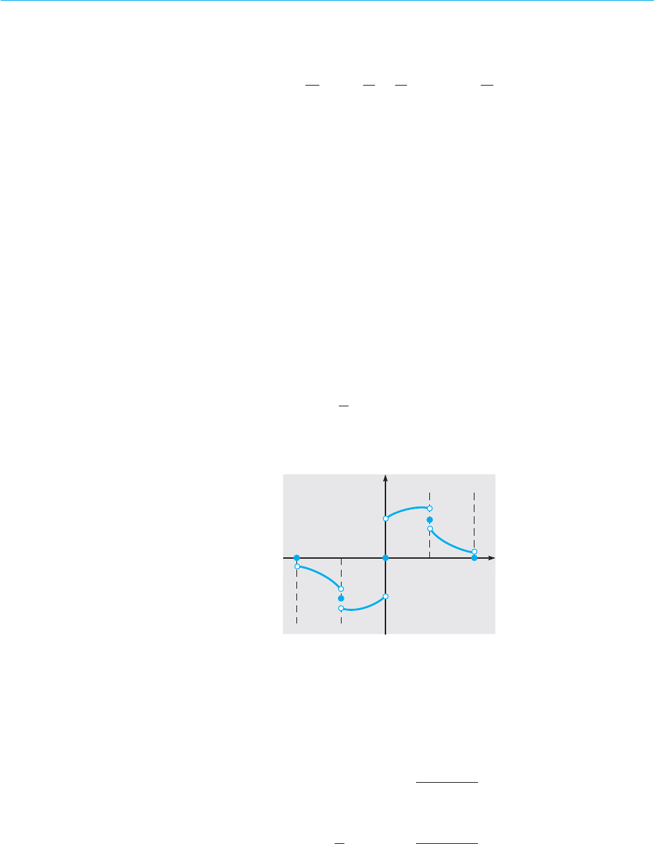
August 7, 2012 21:05 c10 Sheet number 34 Page number 622 cyan black
622 Chapter 10. Partial Differential Equations and Fourier Series
(b) Apply the result of part (a) to the series for the sawtooth wave given in Eq. (9), and
thereby show that
π
2
6
= 1 +
1
2
2
+
1
3
2
+···=
∞
4
n=1
1
n
2
.
This relation was discovered by Euler in about 1735.
More Specialized Fourier Series. Let f be a function originally defined on 0 ≤ x ≤ L and
satisfying there the continuity conditions of Theorem 10.3.1. In this section we have shown
that it is possible to represent f by either a sine series or a cosine series by constructing odd or
even periodic extensions of f , respectively. Problems 38 through 40 concern some other, more
specialized Fourier series that converge to the given function f on (0, L).
38. Let f be extended into (L,2L] in an arbitrary manner subject to the continuity conditions
ofTheorem 10.3.1.Then extend the resulting function into (−2L,0) as an odd function and
elsewhere as a periodic function of period 4L (see Figure 10.4.6). Show that this function
has a Fourier sine series in terms of the functions sin(nπx/2L), n = 1, 2, 3, ...; that is,
f (x) =
∞
4
n=1
b
n
sin(nπx/2L),
where
b
n
=
1
L
"
2L
0
f (x) sin(nπx/2L) dx.
This series converges to the original function on (0, L).
y
x
2
– L–2L
LL
FIGURE 10.4.6 Graph of the function in Problem 38.
39. Let f first be extended into (L,2L) so that it is symmetric about x = L. Then f satisfies
f (2L − x) = f (x) for 0 ≤ x < L. Let the resulting function be extended into (−2L,0) as an
odd function and elsewhere as a periodic function of period 4L (see Figure 10.4.7). Show
that this function has a Fourier series in terms of the functions sin(πx/2L), sin(3πx/2L),
sin(5πx/2L), ...; that is,
f (x) =
∞
4
n=1
b
n
sin
(2n − 1)πx
2L
,
where
b
n
=
2
L
"
L
0
f (x) sin
(2n − 1)πx
2L
dx.
This series converges to the original function on (0, L].

August 7, 2012 21:05 c10 Sheet number 35 Page number 623 cyan black
10.5 Separation of Variables; Heat Conduction in a Rod 623
y
x
2LL– L
–2L
FIGURE 10.4.7 Graph of the function in Problem 39.
40. (a) How should f , originally defined on [0, L], be extended so as to obtain a Fourier
series involving only the functions cos(πx/2L), cos(3πx/2L), cos(5πx/2L), ...? Refer to
Problems 38 and 39.
(b) If f (x) = x for 0 ≤ x ≤ L, sketch the function to which the Fourier series converges
for −4L ≤ x ≤ 4L.
10.5 Separation of Variables; Heat Conduction in a Rod
The basic partial differential equations of heat conduction, wave propagation, and
potential theory that we discuss in this chapter are associated with three distinct
types of physical phenomena: diffusive processes, oscillatory processes, and time-
independent or steady processes. Consequently, they are of fundamental importance
in many branches of physics. They are also of considerable significance from a
mathematical point of view. The partial differential equations whose theory is best
developed and whose applications are most significant and varied are the linear
equations of second order. All such equations can be classified into one of three cat-
egories:the heat conduction equation,the wave equation,and the potential equation,
respectively,are prototypes of these categories.Thus a study of these three equations
yields much information about more general second order linear partial differential
equations.
During the last two centuries, several methods have been developed for solving
partial differential equations. The method of separation of variables is the oldest
systematic method, having been used by D’Alembert, Daniel Bernoulli, and Euler
about 1750 in their investigations of waves and vibrations. It has been considerably
refined and generalized in the meantime,and it remainsa methodof great importance
and frequent use today. To show how the method of separation of variables works,
we considerfirst abasic problemof heat conduction in a solid body.The mathematical
study of heat conduction originated
9
about 1800, and it continues to command the
attention of modern scientists. For example, analysis of the dissipation and transfer
9
The first important investigation of heat conduction was carried out by Joseph Fourier. He presented basic
papers on the subject to the Academy of Sciences of Paris in 1807 and 1811. Although these papers were
controversial and were not published at the time, Fourier continued to develop his ideas and eventually
wrote one of the classics of applied mathematics,Théorie analytique de la chaleur, published in 1822.

August 7, 2012 21:05 c10 Sheet number 36 Page number 624 cyan black
624 Chapter 10. Partial Differential Equations and Fourier Series
of heat away from its sources in high-speed machinery is frequently an important
technological problem.
Let us now consider a heat conduction problem for a straight bar of uniform cross
section and homogeneous material. Let the x-axis be chosen to lie along the axis
of the bar, and let x = 0 and x = L denote the ends of the bar (see Figure 10.5.1).
Suppose further that the sides of the bar are perfectly insulated so that no heat passes
through them. We also assume that the cross-sectional dimensions are so small that
the temperature u can be considered constant on any given cross section. Then u is
a function only of the axial coordinate x and the time t.
x
u(x, t)
x = 0 x = L
FIGURE 10.5.1 A heat-conducting solid bar.
The variation of temperature in the bar is governed by a partial differential
equation whose derivation appears in Appendix A at the end of this chapter. The
equation is called the heat conduction equation and has the form
α
2
u
xx
= u
t
,0< x < L, t > 0, (1)
where α
2
is a constant known as the thermal diffusivity. The parameter α
2
depends
only on the material from which the bar is made and is defined by
α
2
= κ/ρs, (2)
where κ is the thermal conductivity, ρ is the density, and s is the specific heat of the
material in the bar. The units of α
2
are (length)
2
/time. Typical values of α
2
are given
in Table 10.5.1.
TABLE 10.5.1 Values of the Thermal
Diffusivity for Some Common
Materials
Material α
2
(cm
2
/s)
Silver 1.71
Copper 1.14
Aluminum 0.86
Cast iron 0.12
Granite 0.011
Brick 0.0038
Water 0.00144
In addition, we assume that the initial temperature distribution in the bar is given;
thus
u(x,0) = f (x),0≤ x ≤ L, (3)
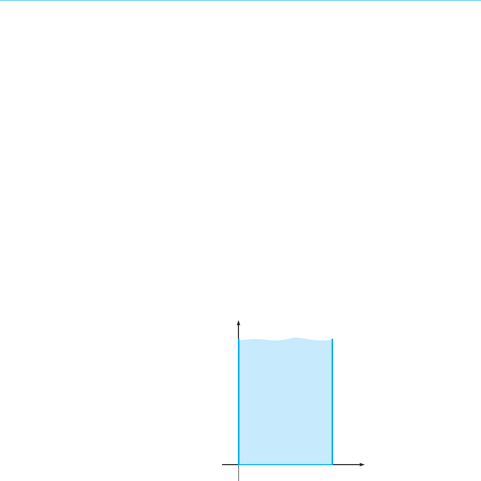
August 7, 2012 21:05 c10 Sheet number 37 Page number 625 cyan black
10.5 Separation of Variables; Heat Conduction in a Rod 625
where f is a given function. Finally,we assume that the ends of thebar are held at fixed
temperatures: the temperature T
1
at x = 0 and the temperature T
2
at x = L. How-
ever, it turns out that we need only consider the case where T
1
= T
2
= 0. We show
in Section 10.6 how to reduce the more general problem to this special case. Thus, in
this section we will assume that u is always zero when x = 0 or x = L:
u(0, t) = 0, u(L, t) = 0, t > 0. (4)
The fundamental problem of heat conduction is to find u(x, t) that satisfies the differ-
ential equation (1) for 0 < x < L and for t > 0, the initial condition (3) when t = 0,
and the boundary conditions (4) at x = 0 and x = L.
The problem described by Eqs. (1), (3), and (4) is an initial value problem in the
time variable t; an initial condition is given, and the differential equation governs
what happens later. However, with respect to the space variable x, the problem is
a boundary value problem; boundary conditions are imposed at each end of the
bar, and the differential equation describes the evolution of the temperature in the
interval between them. Alternatively, we can consider the problem as a boundary
value problem in the xt-plane (see Figure 10.5.2). The solution u(x, t) of Eq. (1) is
sought in the semi-infinite strip 0 < x < L, t > 0, subject to the requirement that
u(x, t) must assume a prescribed value at each point on the boundary of this strip.
x
t
x = L
u(0, t) = 0
u(x,0) = f (x)
u(L, t) = 0
2
u
xx
= u
t
α
FIGURE 10.5.2 Boundary value problem for the heat conduction equation.
The heat conduction problem (1), (3), (4) is linear since u appears only to the
first power throughout. The differential equation and boundary conditions are also
homogeneous.This suggests thatwe might approachthe problem byseeking solutions
of the differential equation and boundary conditions, and then superposing them to
satisfy the initial condition. The remainder of this section describes how this plan can
be implemented.
Method of Separation of Variables. One solution of the differential equation (1) that sat-
isfies the boundary conditions (4) is the function u(x, t) = 0, but this solution does
not satisfy the initial condition (3) except in the trivial case in which f (x) is also zero.

August 7, 2012 21:05 c10 Sheet number 38 Page number 626 cyan black
626 Chapter 10. Partial Differential Equations and Fourier Series
Thus our goal is to find other, nonzero solutions of the differential equation and
boundary conditions.To find the needed solutions,we start by making a basic assump-
tion about the form of the solutions that has far-reaching, and perhaps unforeseen,
consequences. The assumption is that u(x, t) is a product of two functions, one
depending only on x and the other depending only on t; thus
u(x, t) = X(x)T(t). (5)
We will simplify the following derivation by often omitting the independent variables
x and t; our notation is intended to indicate that the functions X and T depend on
the variables x and t, respectively.
Substituting from Eq. (5) for u in the differential equation (1) yields
α
2
X
′′
T = XT
′
, (6)
where primes refer to ordinary differentiation with respect to the independent
variable, whether x or t. Equation (6) is equivalent to
X
′′
X
=
1
α
2
T
′
T
, (7)
in which the variables are separated; that is, the left side depends only on x and the
right side only on t.
It is now crucial to realize that for Eq. (7) to be valid for 0 < x < L, t > 0, it is
necessary that both sides of Eq. (7) must be equal to the same constant. Otherwise,
if one independent variable (say, x) were kept fixed and the other were allowed to
vary, one side (the left in this case) of Eq. (7) would remain unchanged while the
other varied, thus violating the equality. If we call this separation constant −λ, then
Eq. (7) becomes
X
′′
X
=
1
α
2
T
′
T
=−λ. (8)
Hence we obtain the following two ordinary differential equations for X(x) and T(t):
X
′′
+ λX = 0, (9)
T
′
+ α
2
λT = 0. (10)
We denote the separation constant by −λ (rather than λ) because in this problem
it turns out that it must be negative, and it is convenient to exhibit the minus sign
explicitly.
The assumption (5) has led to the replacement of the partial differential equation
(1) by the two ordinary differential equations (9) and (10). Each of these equations is
linear and homogeneous, with constant coefficients, and so can be readily solved for
any value of λ.The product of two solutions of Eq. (9) and (10),respectively,provides
a solution of the partial differential equation (1). However, we are interested only in
those solutions of Eq. (1) that also satisfy the boundary conditions (4). As we now
show, this severely restricts the possible values of λ.
Substituting for u(x, t) from Eq. (5) in the boundary condition at x = 0, we obtain
u(0, t) = X(0)T(t) = 0. (11)

August 7, 2012 21:05 c10 Sheet number 39 Page number 627 cyan black
10.5 Separation of Variables; Heat Conduction in a Rod 627
If Eq. (11) is satisfied by choosing T(t) to be zero for all t, then u(x , t) is zero for
all x and t, and we have already rejected this possibility. Therefore, Eq. (11) must be
satisfied by requiring that
X(0) = 0. (12)
Similarly, the boundary condition at x = L requires that
X(L) = 0. (13)
We now want to consider Eq. (9) subject to the boundary conditions (12) and (13).
This is an eigenvalue problem and, in fact, is the same problem that we discussed in
detail at the end of Section 10.1; see especially the paragraph following Eq. (29) in
that section. The only difference is that the dependent variable there was called y
rather than X. If we refer to the results obtained earlier [Eq. (31) of Section 10.1],
the only nontrivial solutions of Eqs. (9), (12), and (13) are the eigenfunctions
X
n
(x) = sin(nπx/L), n = 1, 2, 3,... (14)
associated with the eigenvalues
λ
n
= n
2
π
2
/L
2
, n = 1, 2, 3, .... (15)
Turning now to Eq. (10) for T(t) and substituting n
2
π
2
/L
2
for λ, we have
T
′
+ (n
2
π
2
α
2
/L
2
)T = 0. (16)
Thus T(t) is proportional to exp(−n
2
π
2
α
2
t/L
2
). Hence, multiplying solutions of
Eqs. (9) and (10) together, and neglecting arbitrary constants of proportionality, we
conclude that the functions
u
n
(x, t) = e
−n
2
π
2
α
2
t/L
2
sin(nπx/L), n = 1, 2, 3,... (17)
satisfy the partial differential equation (1) and the boundary conditions (4) for each
positive integer value of n. The functions u
n
are sometimes called fundamental
solutions of the heat conduction problem (1), (3), and (4).
It remains only to satisfy the initial condition (3):
u(x,0) = f (x),0≤ x ≤ L. (18)
Recall that we have often solved an initial value problem by using the principle of
superposition; that is, we form a linear combination of a set of fundamental solutions
of the differential equation and then choose the coefficients to satisfy the initial
conditions.The analogous step in the present problem is to form a linear combination
of the functions (17) and then to choose the coefficients to satisfy Eq. (18). The main
difference from earlier problems is that there are infinitely many functions (17), so a
general linear combination of them is an infinite series. Thus we assume that
u(x, t) =
∞
4
n=1
c
n
u
n
(x, t) =
∞
4
n=1
c
n
e
−n
2
π
2
α
2
t/L
2
sin
nπx
L
, (19)
where the coefficients c
n
are as yet undetermined. The individual terms in the series
(19) satisfy the differential equation (1) and boundary conditions (4).We will assume

August 7, 2012 21:05 c10 Sheet number 40 Page number 628 cyan black
628 Chapter 10. Partial Differential Equations and Fourier Series
that the infinite series of Eq. (19) converges and also satisfies Eqs. (1) and (4). To
satisfy the initial condition (3), we must have
u(x,0) =
∞
4
n=1
c
n
sin
nπx
L
= f (x). (20)
In other words,weneed to choosethe coefficients c
n
so that theseries of sinefunctions
in Eq. (20) converges to the initial temperature distribution f (x) for 0 ≤ x ≤ L. The
series in Eq. (20) is just the Fourier sine series for f ; according to Eq. (8) of Section
10.4, its coefficients are given by
c
n
=
2
L
"
L
0
f (x) sin
nπx
L
dx. (21)
Hence the solution of the heat conduction problem of Eqs. (1), (3), and (4) is given
by the series in Eq. (19) with the coefficients computed from Eq. (21).
EXAMPLE
1
Find the temperature u(x, t) at any time in a metal rod 50 cm long,insulated on the sides,which
initially has a uniform temperature of 20
◦
C throughout and whose ends are maintained at 0
◦
C
for all t > 0.
The temperature in the rod satisfies the heat conduction problem (1), (3), (4) with L = 50
and f (x) = 20 for 0 < x < 50. Thus, from Eq. (19), the solution is
u(x, t) =
∞
4
n=1
c
n
e
−n
2
π
2
α
2
t/2500
sin
nπx
50
, (22)
where, from Eq. (21),
c
n
=
4
5
"
50
0
sin
nπx
50
dx =
40
nπ
(1 − cos nπ) =
2
80/nπ, n odd;
0, n even.
(23)
Finally, by substituting for c
n
in Eq. (22), we obtain
u(x, t) =
80
π
∞
4
n=1,3,5,...
1
n
e
−n
2
π
2
α
2
t/2500
sin
nπx
50
. (24)
The expression (24) for the temperature is moderately complicated, but the negative expo-
nential factor in each term of the series causes the series to converge quite rapidly, except for
small values of t or α
2
. Therefore, accurate results can usually be obtained by using only the
first few terms of the series.
In order to display quantitative results, let us measure t in seconds; then α
2
has the units
of cm
2
/s. If we choose α
2
= 1 for convenience, this corresponds to a rod of a material whose
thermal properties are somewhere between copper and aluminum. The behavior of the solu-
tion can be seen from the graphs in Figures 10.5.3 through 10.5.5. In Figure 10.5.3 we show
the temperature distribution in the bar at several different times. Observe that the tempera-
ture diminishes steadily as heat in the bar is lost through the end points. The way in which the
temperature decays at a given point in the bar is indicated in Figure 10.5.4,where temperature
is plotted against time for a few selected points in the bar. Finally, Figure 10.5.5 is a three-
dimensional plot of u versus both x and t. Observe that we obtain the graphs in Figures 10.5.3

August 7, 2012 21:05 c10 Sheet number 41 Page number 629 cyan black
10.5 Separation of Variables; Heat Conduction in a Rod 629
5020 30 0401
20
15
10
5
u
x
t = 0
t = 20
t = 50
t = 150
t = 300
FIGURE 10.5.3 Temperature distributions at several times
for the heat conduction problem of Example 1.
500200 300 004001
20
15
10
5
u
t
x = 5
x = 15
x = 25
FIGURE 10.5.4 Dependence of temperature on time at several locations
for the heat conduction problem of Example 1.
and 10.5.4 by intersecting the surface in Figure 10.5.5 by planes on which either t or x is con-
stant. The slight waviness in Figure 10.5.5 at t = 0 results from using only a finite number of
terms in the series for u(x, t) and from the slow convergence of the series for t = 0.
A problem with possible practical implications is to determine the time τ at which the
entire bar has cooled to a specified temperature. For example, when is the temperature in
the entire bar no greater than 1
◦
C? Because of the symmetry of the initial temperature distri-
bution and the boundary conditions, the warmest point in the bar is always the center. Thus τ
is found by solving u(25, t) = 1 for t. Using one term in the series expansion (24), we obtain
τ =
2500
π
2
ln(80/π)
∼
=
820 s.

August 7, 2012 21:05 c10 Sheet number 42 Page number 630 cyan black
630 Chapter 10. Partial Differential Equations and Fourier Series
20
15
10
5
5010
20
30
40
50
100
150
200
250
t
u
x
FIGURE 10.5.5 Plot of temperature u versus x and t for
the heat conduction problem of Example 1.
PROBLEMS In each of Problems 1 through 6, determine whether the method of separation of variables
can be used to replace the given partial differential equation by a pair of ordinary differential
equations. If so, find the equations.
1. xu
xx
+ u
t
= 02.tu
xx
+ xu
t
= 0
3. u
xx
+ u
xt
+ u
t
= 04.[p(x)u
x
]
x
− r(x)u
tt
= 0
5. u
xx
+ (x + y)u
yy
= 06.u
xx
+ u
yy
+ xu = 0
7. Find the solution of the heat conduction problem
100u
xx
= u
t
,0< x < 1, t > 0;
u(0, t) = 0, u(1, t) = 0, t > 0;
u(x,0) = sin 2πx − sin 5πx,0≤ x ≤ 1.
8. Find the solution of the heat conduction problem
u
xx
= 4u
t
,0< x < 2, t > 0;
u(0, t) = 0, u(2, t) = 0, t > 0;
u(x,0) = 2 sin(πx/2) − sin πx + 4 sin 2πx,0≤ x ≤ 2.
Consider the conduction of heat in a rod 40 cm in length whose ends are maintained at 0
◦
C
for all t > 0. In each of Problems 9 through 12, find an expression for the temperature u(x, t)
if the initial temperature distribution in the rod is the given function. Suppose that α
2
= 1.
9. u(x,0) = 50, 0 < x < 40
10. u(x,0) =
2
x,0≤ x < 20,
40 − x,20≤ x ≤ 40

August 7, 2012 21:05 c10 Sheet number 43 Page number 631 cyan black
10.5 Separation of Variables; Heat Conduction in a Rod 631
11. u(x,0) =
⎧
⎪
⎨
⎪
⎩
0, 0 ≤ x < 10,
50, 10 ≤ x ≤ 30,
0, 30 < x ≤ 40
12. u(x,0) = x,0< x < 40
13.
Consider again the rod in Problem 9. For t = 5 and x = 20, determine how many terms are
needed to find the solution correct to three decimal places. A reasonable way to do this is
to find n so that including one more term does not change the first three decimal places of
u(20, 5). Repeat for t = 20 and t = 80. Form a conclusion about the speed of convergence
of the series for u(x, t).
14.
For the rod in Problem 9:
(a) Plot u versus x for t = 5, 10, 20, 40, 100, and 200. Put all of the graphs on the same
set of axes and thereby obtain a picture of the way in which the temperature distribution
changes with time.
(b) Plot u versus t for x = 5, 10, 15, and 20.
(c) Draw a three-dimensional plot of u versus x and t.
(d) How long does it take for the entire rod to cool off to a temperature of no more than
1
◦
C?
15.
Follow the instructions in Problem 14 for the rod in Problem 10.
16.
Follow the instructions in Problem 14 for the rod in Problem 11.
17.
For the rod in Problem 12:
(a) Plot u versus x for t = 5, 10, 20, 40, 100, and 200.
(b) For each value of t used in part (a), estimate the value of x for which the temperature
is greatest. Plot these values versus t to see how the location of the warmest point in the
rod changes with time.
(c) Plot u versus t for x = 10, 20, and 30.
(d) Draw a three-dimensional plot of u versus x and t.
(e) How long does it take the entire rod to cool to a temperature of no more than 1
◦
C?
18.
Let a metallic rod 20 cm long be heated to a uniform temperature of 100
◦
C. Suppose that
at t = 0, the ends of the bar are plunged into an ice bath at 0
◦
C and thereafter maintained
at this temperature, but that no heat is allowed to escape through the lateral surface. Find
an expression for the temperature at any point in the bar at any later time. Determine the
temperature at the center of the bar at time t = 30 s if the bar is made (a) of silver, (b) of
aluminum, (c) of cast iron.
19.
For the rod of Problem 18, find the time that will elapse before the center of the bar cools
to a temperature of 5
◦
C if the bar is made (a) of silver, (b) of aluminum, (c) of cast iron.
20. In solving differential equations, the computations can almost always be simplified by the
use of dimensionless variables.
(a) Show that if the dimensionless variable ξ = x/L is introduced, the heat conduction
equation becomes
∂
2
u
∂ξ
2
=
L
2
α
2
∂u
∂t
,0<ξ<1, t > 0.
(b) Since L
2
/α
2
has the units of time, it is convenient to use this quantity to define a di-
mensionless time variable τ = (α
2
/L
2
)t. Then show that the heat conduction equation

August 7, 2012 21:05 c10 Sheet number 44 Page number 632 cyan black
632 Chapter 10. Partial Differential Equations and Fourier Series
reduces to
∂
2
u
∂ξ
2
=
∂u
∂τ
,0<ξ<1, τ>0.
21. Consider the equation
au
xx
− bu
t
+ cu = 0, (i)
where a, b, and c are constants.
(a) Let u(x, t) = e
δt
w(x, t), where δ is constant, and find the corresponding partial
differential equation for w.
(b) If b ̸= 0, show that δ can be chosen so that the partial differential equation found in
part (a) has no term in w. Thus, by a change of dependent variable, it is possible to reduce
Eq. (i) to the heat conduction equation.
22. The heat conduction equation in two space dimensions is
α
2
(u
xx
+ u
yy
) = u
t
.
Assuming that u(x, y, t) = X(x)Y(y)T(t), find ordinary differential equations that are
satisfied by X (x), Y(y), and T(t).
23. The heat conduction equation in two space dimensions may be expressed in terms of polar
coordinates as
α
2
[u
rr
+ (1/r)u
r
+ (1/r
2
)u
θθ
]=u
t
.
Assuming that u(r, θ, t) = R(r);(θ)T(t), find ordinary differential equations that are
satisfied by R(r), ;(θ), and T(t).
10.6 Other Heat Conduction Problems
In Section10.5 we considered the problem consisting ofthe heat conduction equation
α
2
u
xx
= u
t
,0< x < L, t > 0, (1)
the boundary conditions
u(0, t) = 0, u(L, t) = 0, t > 0, (2)
and the initial condition
u(x,0) = f (x),0≤ x ≤ L. (3)
We found the solution to be
u(x, t) =
∞
4
n=1
c
n
e
−n
2
π
2
α
2
t/L
2
sin
nπx
L
, (4)
where the coefficients c
n
are the same as in the series
f (x) =
∞
4
n=1
c
n
sin
nπx
L
. (5)

August 7, 2012 21:05 c10 Sheet number 45 Page number 633 cyan black
10.6 Other Heat Conduction Problems 633
The series in Eq. (5) is just the Fourier sine series for f ; according to Section 10.4, its
coefficients are given by
c
n
=
2
L
"
L
0
f (x) sin
nπx
L
dx. (6)
Hence the solution of the heat conduction problem, Eqs. (1) to (3), is given by the
series in Eq. (4) with the coefficients computed from Eq. (6).
We emphasize that, at this stage, the solution (4) must be regarded as a formal
solution;that is,we obtained it without rigorous justification of the limiting processes
involved. Such a justification is beyond the scope of this book. However, once the
series (4) has been obtained, it is possible to show that in 0 < x < L, t > 0, it con-
verges to a continuous function; that the derivatives u
xx
and u
t
can be computed
by differentiating the series (4) term by term; and that the heat conduction equa-
tion (1) is indeed satisfied. The argument relies heavily on the fact that each term
of the series (4) contains a negative exponential factor, and this results in relatively
rapid convergence of the series. A further argument establishes that the function u
given by Eq. (4) also satisfies the boundary and initial conditions; this completes the
justification of the formal solution.
It is interesting to note that although f satisfies the conditions of the Fourier con-
vergence theorem (Theorem 10.3.1), it may have points of discontinuity. In this case
the initial temperature distribution u(x,0) = f (x) is discontinuous at one or more
points. Nevertheless, the solution u(x, t) is continuous for arbitrarily small values of
t > 0. This illustrates the fact that heat conduction is a diffusive process that instantly
smooths out any discontinuities that may be present in the initial temperature dis-
tribution. Finally, since f is bounded, it follows from Eq. (6) that the coefficients c
n
are also bounded. Consequently, the presence of the negative exponential factor in
each term of the series (4) guarantees that
lim
t→∞
u(x, t) = 0 (7)
for all x regardless of the initial condition. This is in accord with the result expected
from physical intuition.
We now consider two other problems of one-dimensional heat conduction that can
be handled by the method developed in Section 10.5.
Nonhomogeneous Boundary Conditions. Suppose now that one end of the bar is held at a
constant temperature T
1
and the other is maintained at a constant temperature T
2
.
Then the boundary conditions are
u(0, t) = T
1
, u(L, t) = T
2
, t > 0. (8)
The differential equation (1) and the initial condition (3) remain unchanged.
This problem is only slightly more difficult, because of the nonhomogeneous
boundary conditions, than the one in Section 10.5. We can solve it by reducing it
to a problem having homogeneous boundary conditions, which can then be solved
as in Section 10.5. The technique for doing this is suggested by the following physical
argument.
After a long time—that is, as t →∞—we anticipate that a steady temperature
distribution v(x) will be reached, which is independent of the time t and the initial

August 7, 2012 21:05 c10 Sheet number 46 Page number 634 cyan black
634 Chapter 10. Partial Differential Equations and Fourier Series
conditions. Since v(x) does not depend on t, its time derivative v
t
is zero; the heat
conduction equation (1) for v then becomes
v
′′
(x) = 0, 0 < x < L. (9)
Hence the steady state temperature distribution is a linear function of x. Further,
v(x) must satisfy the boundary conditions
v(0) = T
1
, v(L) = T
2
, (10)
which are valid even as t →∞. The solution of Eq. (9) satisfying Eqs. (10) is
v(x) = (T
2
− T
1
)
x
L
+ T
1
. (11)
Returning to the original problem,Eqs. (1),(3),and (8),we will try to express u(x, t)
as the sum of the steady state temperature distribution v(x) and another (transient)
temperature distribution w(x, t); thus we write
u(x, t) = v(x) + w(x, t). (12)
Since v(x) is given by Eq. (11), the problem will be solved provided that we can
determine w(x, t). The boundary value problem for w(x, t) is found by substituting
the expression in Eq. (12) for u(x, t) in Eqs. (1), (3), and (8).
From Eq. (1) we have
α
2
(v + w)
xx
= (v + w)
t
;
it follows that
α
2
w
xx
= w
t
, (13)
since v
xx
= 0 and v
t
= 0. Similarly, from Eqs. (12), (8), and (10),
w(0, t) = u(0, t) − v(0) = T
1
− T
1
= 0,
(14)
w(L, t) = u(L, t) − v(L) = T
2
− T
2
= 0.
Finally, from Eqs. (12) and (3),
w(x,0) = u(x,0) − v(x) = f (x) − v(x), (15)
where v(x) is given by Eq. (11). Thus the transient part of the solution to the original
problem is found by solving the problem consisting of Eqs. (13), (14), and (15). This
latter problem is precisely the one solved in Section 10.5, provided that f (x) − v(x)
is now regarded as the initial temperature distribution. Hence
u(x, t) = (T
2
− T
1
)
x
L
+ T
1
+
∞
4
n=1
c
n
e
−n
2
π
2
α
2
t/L
2
sin
nπx
L
, (16)
where
c
n
=
2
L
"
L
0
;
f (x) − (T
2
− T
1
)
x
L
− T
1
<
sin
nπx
L
dx. (17)
This is another case in which a more difficult problem is solved by reducing it to a
simpler problem that has already been solved. The technique of reducing a problem
with nonhomogeneous boundary conditions to one with homogeneous boundary
conditions by subtracting the steady state solution has wide application.

August 7, 2012 21:05 c10 Sheet number 47 Page number 635 cyan black
10.6 Other Heat Conduction Problems 635
EXAMPLE
1
Consider the heat conduction problem
u
xx
= u
t
,0< x < 30, t > 0, (18)
u(0, t) = 20, u(30, t) = 50, t > 0, (19)
u(x,0) = 60 − 2x,0< x < 30. (20)
Find the steady state temperature distribution and the boundary value problem that
determines the transient distribution.
The steady state temperature satisfies v
′′
(x) = 0 and the boundary conditions v(0) = 20 and
v(30) = 50. Thus v(x) = 20 + x. The transient distribution w(x, t) satisfies the heat conduction
equation
w
xx
= w
t
, (21)
the homogeneous boundary conditions
w(0, t) = 0, w(30, t) = 0, (22)
and the modified initial condition
w(x,0) = 60 − 2x − (20 + x ) = 40 − 3x. (23)
Note that this problem is of the form (1), (2), (3) with f (x) = 40 − 3x , α
2
= 1, and L = 30. Thus
the solution is given by Eqs. (4) and (6).
Figure 10.6.1 shows a plot of the initial temperature distribution 60 − 2x, the final temper-
ature distribution 20 + x, and the temperature at three intermediate times found by solving
Eqs. (21) through (23). Note that the intermediate temperature satisfies the boundary condi-
tions (19) for any t > 0. As t increases, the effect of the boundary conditions gradually moves
from the ends of the bar toward its center.
10
20
30
40
50
60
10 510252350
u
x
t = 0
t = 30
t = 10
t = 2
t →
∞
FIGURE 10.6.1 Temperature distributions at several times
for the heat conduction problem of Example 1.
Bar with Insulated Ends. A slightly different problem occurs if the ends of the bar are
insulated so that there is no passage of heat through them. According to Eq. (2) in
Appendix A, the rate of flow of heat across a cross section is proportional to the rate

August 7, 2012 21:05 c10 Sheet number 48 Page number 636 cyan black
636 Chapter 10. Partial Differential Equations and Fourier Series
of change of temperature in the x direction. Thus, in the case of no heat flow, the
boundary conditions are
u
x
(0, t) = 0, u
x
(L, t) = 0, t > 0. (24)
The problem posed by Eqs. (1), (3), and (24) can also be solved by the method of
separation of variables. If we let
u(x, t) = X(x)T(t), (25)
and substitute for u in Eq. (1), then it follows, as in Section 10.5, that
X
′′
X
=
1
α
2
T
′
T
=−λ, (26)
where λ is a constant. Thus we obtain again the two ordinary differential equations
X
′′
+ λX = 0, (27)
T
′
+ α
2
λT = 0. (28)
For any value of λ, a product of solutions of Eqs. (27) and (28) is a solution of the
partial differential equation (1). However, we are interested only in those solutions
that also satisfy the boundary conditions (24).
If we substitute for u(x, t) from Eq. (25) in the boundary condition at x = 0, we
obtain X
′
(0)T(t) = 0. We cannot permit T(t) to be zero for all t, since then u(x, t)
would also be zero for all t. Hence we must have
X
′
(0) = 0. (29)
Proceeding in the same way with the boundary condition at x = L, we find that
X
′
(L) = 0. (30)
Thus we wish to solve Eq. (27) subject to the boundary conditions (29) and (30). It
is possible to show that nontrivial solutions of this problem can exist only if λ is real.
One way to show this is indicated in Problem 18; alternatively, we can appeal to a
more general theory to be discussed in Section 11.2. We will assume that λ is real and
will consider in turn the three cases λ<0, λ = 0, and λ>0.
If λ<0, we let λ =−µ
2
, where µ is real and positive, so that Eq. (27) becomes
X
′′
− µ
2
X = 0. It is convenient to write its general solution as
X(x) = k
1
sinh µx + k
2
cosh µx (31)
so that the boundary conditions are easier to apply. In this case the boundary con-
ditions can be satisfied only by choosing k
1
= k
2
= 0. Since this is unacceptable, it
follows that λ cannot be negative; in other words, the problem (27), (29), (30) has no
negative eigenvalues.
If λ = 0, then Eq. (27) is X
′′
= 0, and therefore,
X(x) = k
1
x + k
2
. (32)
The boundary conditions (29) and (30) require that k
1
= 0 but do not determine k
2
.
Thus λ = 0 is an eigenvalue,corresponding to the eigenfunction X (x) = 1. For λ = 0,
it follows from Eq. (28) that T(t) is also a constant, which can be combined with k
2
.
Hence, for λ = 0, we obtain the constant solution u(x, t) = k
2
.

August 7, 2012 21:05 c10 Sheet number 49 Page number 637 cyan black
10.6 Other Heat Conduction Problems 637
Finally, if λ>0, let λ = µ
2
, where µ is real and positive. Then Eq. (27) becomes
X
′′
+ µ
2
X = 0, and consequently,
X(x) = k
1
sin µx + k
2
cos µx. (33)
The boundary condition (29) requires that k
1
= 0, and the boundary condition (30)
requires that µ = nπ/L for n = 1, 2, 3, ... but leaves k
2
arbitrary. Thus the problem
(27), (29),(30) has an infinite sequence of positive eigenvalues λ = n
2
π
2
/L
2
with the
correspondingeigenfunctions X(x) = cos(nπx/L). Forthese valuesof λ,thesolutions
T(t) of Eq. (28) are proportional to exp(−n
2
π
2
α
2
t/L
2
).
Combining all these results, we have the following fundamental solutions for the
problem (1), (3), and (24):
u
0
(x, t) = 1,
(34)
u
n
(x, t) = e
−n
2
π
2
α
2
t/L
2
cos
nπx
L
, n = 1, 2, ...,
where arbitrary constants of proportionality have been dropped. Each of these func-
tions satisfies the differential equation (1) and the boundary conditions (24). Because
both the differential equation and the boundary conditions are linear and homoge-
neous, any finite linear combination of the fundamental solutions satisfies them. We
will assume that this is true for convergent infinite linear combinations of fundamen-
tal solutions as well. Thus, to satisfy the initial condition (3), we assume that u(x , t)
has the form
u(x, t) =
c
0
2
u
0
(x, t) +
∞
4
n=1
c
n
u
n
(x, t)
=
c
0
2
+
∞
4
n=1
c
n
e
−n
2
π
2
α
2
t/L
2
cos
nπx
L
. (35)
The coefficients c
n
are determined by the requirement that
u(x,0) =
c
0
2
+
∞
4
n=1
c
n
cos
nπx
L
= f (x). (36)
Thus the unknown coefficients in Eq. (35) must be the coefficients in the Fourier
cosine series of period 2L for f . Hence
c
n
=
2
L
"
L
0
f (x) cos
nπx
L
dx, n = 0, 1, 2, .... (37)
With this choice of the coefficients c
0
, c
1
, c
2
, ..., the series (35) provides the solution
to the heat conduction problem for a rod with insulated ends, Eqs. (1), (3), and (24).
It is worth observing that the solution (35) can also be thought of as the sum
of a steady state temperature distribution (given by the constant c
0
/2), which is
independent of time t, and a transient distribution (given by the rest of the infinite
series) that approaches zero in the limit as t approaches infinity. That the steady state
is a constant is consistent with the expectation that the process of heat conduction
will gradually smooth out the initial temperature distribution in the bar as long as no

August 7, 2012 21:05 c10 Sheet number 50 Page number 638 cyan black
638 Chapter 10. Partial Differential Equations and Fourier Series
heat is allowed to enter from, or to escape to, the outside. The physical interpretation
of the term
c
0
2
=
1
L
"
L
0
f (x) dx (38)
is that it is the mean value of the original temperature distribution.
EXAMPLE
2
Find the temperature u(x, t) in a metal rod of length 25 cm that is insulated on the ends as well
as on the sides and whose initial temperature distribution is u(x,0) = x for 0 < x < 25.
The temperature in the rod satisfies the heat conduction problem (1), (3), (24) with L = 25.
Thus, from Eq. (35), the solution is
u(x, t) =
c
0
2
+
∞
4
n=1
c
n
e
−n
2
π
2
α
2
t/625
cos
nπx
25
, (39)
where the coefficients are determined from Eq. (37). We have
c
0
=
2
25
"
25
0
xdx = 25 (40)
and, for n ≥ 1,
c
n
=
2
25
"
25
0
x cos
nπx
25
dx
= 50(cos nπ −1)/(nπ)
2
=
2
−100/(nπ)
2
, n odd;
0, n even.
(41)
Thus
u(x, t) =
25
2
−
100
π
2
∞
4
n=1,3,5,...
1
n
2
e
−n
2
π
2
α
2
t/625
cos(nπx/25) (42)
is the solution of the given problem.
For α
2
= 1, Figure 10.6.2 shows plots of the temperature distribution in the bar at several
times. Again, the convergence of the series is rapid so that only a relatively few terms are
needed to generate the graphs.
2510 15 025
25
20
15
10
5
u
x
t = 0
t = 10
t = 40
t = 100
t →
∞
FIGURE 10.6.2 Temperature distributions at several times
for the heat conduction problem of Example 2.

August 7, 2012 21:05 c10 Sheet number 51 Page number 639 cyan black
10.6 Other Heat Conduction Problems 639
More General Problems. The method of separation of variables can also be used to
solve heat conduction problems with boundary conditions other than those given
by Eqs. (8) and Eqs. (24). For example, the left end of the bar might be held at a fixed
temperature T while the other end is insulated. In this case the boundary conditions
are
u(0, t) = T, u
x
(L, t) = 0, t > 0. (43)
The first step in solving this problem is to reduce the given boundary conditions to
homogeneous ones by subtracting the steady state solution. The resulting problem
is solved by essentially the same procedure as in the problems previously consid-
ered. However, the extension of the initial function f outside of the interval [0, L] is
somewhat different from that in any case considered so far (see Problem 15).
A more general type of boundary condition occurs when the rate of heat flow
through the end of the bar is proportional to the temperature. It is shown in
Appendix A that the boundary conditions in this case are of the form
u
x
(0, t) − h
1
u(0, t) = 0, u
x
(L, t) + h
2
u(L, t) = 0, t > 0, (44)
where h
1
and h
2
are nonnegative constants. If we apply the method of separation of
variables to the problem consisting of Eqs. (1), (3), and (44), we find that X(x) must
be a solution of
X
′′
+ λX = 0, X
′
(0) − h
1
X(0) = 0, X
′
(L) + h
2
X(L) = 0, (45)
where λ is the separation constant. Once again it is possible to show that nontrivial
solutions can exist only for certain nonnegative real values of λ, the eigenvalues, but
these values are not given by a simple formula (see Problem 20). It is also possible
to show that the corresponding solutions of Eqs. (45), the eigenfunctions, satisfy an
orthogonality relation and that we can satisfy the initial condition (3) by superposing
solutions of Eqs. (45). However, the resulting series is not included in the discussion
of this chapter. There is a more general theory that covers such problems, and it is
outlined in Chapter 11.
PROBLEMS In each of Problems 1 through 8, find the steady state solution of the heat conduction equation
α
2
u
xx
= u
t
that satisfies the given set of boundary conditions.
1. u(0, t) = 10, u(50, t) = 40 2. u(0, t) = 30, u(40, t) =−20
3. u
x
(0, t) = 0, u(L, t) = 04. u
x
(0, t) = 0, u(L, t) = T
5. u(0, t) = 0, u
x
(L, t) = 06.u(0, t) = T, u
x
(L, t) = 0
7. u
x
(0, t) − u(0, t) = 0, u(L, t) = T 8. u(0, t) = T, u
x
(L, t) + u(L, t) = 0
9.
Let an aluminum rod of length 20 cm be initially at the uniform temperature of 25
◦
C.
Suppose that at time t = 0, the end x = 0 is cooled to 0
◦
C while the end x = 20 is heated
to 60
◦
C, and both are thereafter maintained at those temperatures.
(a) Find the temperature distribution in the rod at any time t.

August 7, 2012 21:05 c10 Sheet number 52 Page number 640 cyan black
640 Chapter 10. Partial Differential Equations and Fourier Series
(b) Plot the initial temperature distribution, the final (steady state) temperature distribu-
tion, and the temperature distributions at two representative intermediate times on the
same set of axes.
(c) Plot u versus t for x = 5, 10, and 15.
(d) Determine how much time must elapse before the temperature at x = 5 cm comes
(and remains) within 1% of its steady state value.
10.
(a) Let the ends of a copper rod 100 cm long be maintained at 0
◦
C. Suppose that the
center of the bar is heated to 100
◦
C by an external heat source and that this situation is
maintained until a steady state results. Find this steady state temperature distribution.
(b) At a time t = 0 [after the steady state of part (a) has been reached],let the heat source
be removed. At the same instant let the end x = 0 be placed in thermal contact with a
reservoir at 20
◦
C, while the other end remains at 0
◦
C. Find the temperature as a function
of position and time.
(c) Plot u versus x for several values of t. Also plot u versus t for several values of x.
(d) What limiting value does the temperature at the center of the rod approach after a
long time? How much time must elapse before the center of the rod cools to within 1
◦
C
of its limiting value?
11.
Consider a rod of length 30 for which α
2
= 1. Suppose the initial temperature distribution
is given by u(x,0) = x(60 − x)/30 and that the boundary conditions are u(0, t) = 30 and
u(30, t) = 0.
(a) Find the temperature in the rod as a function of position and time.
(b) Plot u versus x for several values of t. Also plot u versus t for several values of x.
(c) Plot u versus t for x = 12. Observe that u initially decreases, then increases for a
while, and finally decreases to approach its steady state value. Explain physically why this
behavior occurs at this point.
12.
Consider a uniform rod of length L with an initial temperature given by
u(x,0) = sin(πx/L),0≤ x ≤ L. Assume that both ends of the bar are insulated.
(a) Find the temperature u(x , t).
(b) What is the steady state temperature as t →∞?
(c) Let α
2
= 1 and L = 40. Plot u versus x for several values of t. Also plot u versus t for
several values of x.
(d) Describe briefly how the temperature in the rod changes as time progresses.
13.
Consider a bar of length 40 cm whose initial temperature is given by u(x,0) = x(60 − x)/30.
Suppose that α
2
= 1/4 cm
2
/s and that both ends of the bar are insulated.
(a) Find the temperature u(x , t).
(b) Plot u versus x for several values of t. Also plot u versus t for several values of x.
(c) Determine the steady state temperature in the bar.
(d) Determine how much time must elapsebefore the temperature at x = 40 comes within
1
◦
C of its steady state value.
14.
Consider a bar 30 cm long that is made of a material for which α
2
= 1 and whose ends are
insulated. Suppose that the initial temperature is zero except for the interval 5 < x < 10,
where the initial temperature is 25
◦
C.
(a) Find the temperature u(x , t).
(b) Plot u versus x for several values of t. Also plot u versus t for several values of x.
(c) Plot u(4, t) and u(11, t) versus t. Observe that the points x = 4 and x = 11 are symmet-
rically located with respect to the initial temperature pulse, yet their temperature plots
are significantly different. Explain physically why this is so.

August 7, 2012 21:05 c10 Sheet number 53 Page number 641 cyan black
10.6 Other Heat Conduction Problems 641
15. Consider a uniform bar of length L having an initial temperature distribution given by
f (x),0≤ x ≤ L. Assume that the temperature at the end x = 0 is held at 0
◦
C, while the
end x = L is insulated so that no heat passes through it.
(a) Show that the fundamental solutions of the partial differential equation and boundary
conditions are
u
n
(x, t) = e
−(2n−1)
2
π
2
α
2
t/4L
2
sin[(2n − 1)πx/2L], n = 1, 2, 3, ....
(b) Find a formal series expansion for the temperature u(x, t)
u(x, t) =
∞
4
n=1
c
n
u
n
(x, t)
that also satisfies the initial condition u(x,0) = f (x).
Hint: Even though the fundamental solutions involve only the odd sines, it is still possi-
ble to represent f by a Fourier series involving only these functions. See Problem 39 of
Section 10.4.
16.
In the bar of Problem 15, suppose that L = 30, α
2
= 1, and the initial temperature distri-
bution is f (x) = 30 − x for 0 < x < 30.
(a) Find the temperature u(x , t).
(b) Plot u versus x for several values of t. Also plot u versus t for several values of x.
(c) How does the location x
m
of the warmest point in the bar change as t increases? Draw
a graph of x
m
versus t.
(d) Plot the maximum temperature in the bar versus t.
17.
Suppose that the conditions are as in Problems 15 and 16 except that the boundary
condition at x = 0 is u(0, t) = 40.
(a) Find the temperature u(x , t).
(b) Plot u versus x for several values of t. Also plot u versus t for several values of x.
(c) Compare the plots you obtained in this problem with those from Problem 16. Explain
how the change in the boundary condition at x = 0 causes the observed differences in the
behavior of the temperature in the bar.
18. Consider the problem
X
′′
+ λX = 0, X
′
(0) = 0, X
′
(L) = 0. (i)
Let λ = µ
2
, where µ = ν + iσ with ν and σ real. Show that if σ ̸= 0, then the only solution
of Eqs. (i) is the trivial solution X(x) = 0.
Hint: Use an argument similar to that in Problem 23 of Section 10.1.
19. The right end of a bar of length a with thermal conductivity κ
1
and cross-sectional area A
1
is joined to the left end of a bar of thermal conductivity κ
2
and cross-sectional area A
2
.
The composite bar has a total length L. Suppose that the end x = 0 is held at temperature
zero, while the end x = L is held at temperature T. Find the steady state temperature in
the composite bar, assuming that the temperature and rate of heat flow are continuous at
x = a.
Hint: See Eq. (2) of Appendix A.
20. Consider the problem
α
2
u
xx
= u
t
,0< x < L, t > 0;
u(0, t) = 0, u
x
(L, t) + γu(L, t) = 0, t > 0; (i)
u(x,0) = f (x),0≤ x ≤ L.

August 7, 2012 21:05 c10 Sheet number 54 Page number 642 cyan black
642 Chapter 10. Partial Differential Equations and Fourier Series
(a) Let u(x, t) = X(x)T(t), and show that
X
′′
+ λX = 0, X(0) = 0, X
′
(L) + γX(L) = 0, (ii)
and
T
′
+ λα
2
T = 0,
where λ is the separation constant.
(b) Assume that λ is real, and show that problem (ii) has no nontrivial solutions if λ ≤ 0.
(c) If λ>0, let λ = µ
2
with µ>0. Show that problem (ii) has nontrivial solutions only if
µ is a solution of the equation
µ cos µL + γ sin µL = 0. (iii)
(d) Rewrite Eq. (iii) as tan µL =−µ/γ. Then, by drawing the graphs of y = tan µL and
y =−µL/γL for µ>0 on the same set of axes, show that Eq. (iii) is satisfied by infinitely
many positive values of µ; denote these by µ
1
, µ
2
, ..., µ
n
, ..., ordered in increasing size.
(e) Determine the set of fundamental solutions u
n
(x, t) corresponding to the values µ
n
found in part (d).
An External Heat Source. Consider the heat conduction problem in a bar that is in thermal
contact with an external heat source or sink. Then the modified heat conduction equation is
u
t
= α
2
u
xx
+ s(x), (i)
where the term s(x) describes the effect of the external agency;s(x) is positive for a source and
negative for a sink. Suppose that the boundary conditions are
u(0, t) = T
1
, u(L, t) = T
2
(ii)
and the initial condition is
u(x,0) = f (x). (iii)
Problems 21 through 23 deal with this kind of problem.
21. Write u(x, t) = v(x) + w(x, t), where v and w are the steady state and transient parts of the
solution,respectively. State theboundary value problems that v(x) and w(x, t),respectively,
satisfy. Observe that the problem for w is the fundamental heat conduction problem
discussed in Section 10.5, with a modified initial temperature distribution.
22.
(a) Suppose that α
2
= 1 and s(x ) = k, a constant, in Eq. (i). Find v(x).
(b) Assume that T
1
= 0, T
2
= 0, L = 20, k = 1/5, and that f (x) = 0 for 0 < x < L. Deter-
mine w(x, t). Then plot u(x, t) versus x for several values of t; on the same axes, also plot
the steady state part of the solution v(x).
23.
(a) Let α
2
= 1 and s(x ) = kx/L, where k is a constant, in Eq. (i). Find v(x).
(b) Assume that T
1
= 10, T
2
= 30, L = 20, k = 1/2, and that f (x) = 0 for 0 < x < L.
Determine w(x, t). Then plot u(x, t) versus x for several values of t; on the same axes,
also plot the steady state part of the solution v(x).

August 7, 2012 21:05 c10 Sheet number 55 Page number 643 cyan black
10.7 The Wave Equation: Vibrations of an Elastic String 643
10.7 The Wave Equation: Vibrations of an Elastic String
A second partial differential equation that occurs frequently in applied mathematics
is the wave
10
equation. Some form of this equation, or a generalization of it, almost
inevitably arises in any mathematical analysis of phenomena involving the propaga-
tion of waves in a continuous medium. For example, the studies of acoustic waves,
water waves,electromagnetic waves,and seismic waves are all based on this equation.
Perhaps the easiest situation to visualize occurs in the investigation of mechanical
vibrations. Suppose that an elastic string of length L is tightly stretched between two
supports at the same horizontal level, so that the x-axis lies along the string (see
Figure 10.7.1).
x
u(x, t )
x = 0 x = L
FIGURE 10.7.1 A vibrating string.
The elastic string may be thought of as a guitar string, a guy wire, or possibly an
electric power line. Suppose that the string is set in motion (by plucking,for example)
so that it vibrates in a vertical plane, and let u(x, t) denote the vertical displacement
experienced by the string at the point x at time t. If damping effects, such as air
resistance, are neglected, and if the amplitude of the motion is not too large, then
u(x, t) satisfies the partial differential equation
a
2
u
xx
= u
tt
(1)
in the domain 0 < x < L, t > 0. Equation (1) is known as the one-dimensional wave
equation and is derived in Appendix B at the end of the chapter. The constant
coefficient a
2
appearing in Eq. (1) is given by
a
2
= T/ρ, (2)
where T is the tension (force) in the string, and ρ is the mass per unit length of the
string material. It follows that a has the units of length/time—that is, of velocity. In
Problem 14 it is shown that a is the velocity of propagation of waves along the string.
10
The solution of the wave equation was one of the major mathematical problems of the mid-eighteenth
century. The wave equation was first derived and studied by D’Alembert in 1746. It also attracted the
attention of Euler (1748), Daniel Bernoulli (1753), and Lagrange (1759). Solutions were obtained in
several different forms, and the merits of, and relations among, these solutions were argued, sometimes
heatedly, in a series of papers extending over more than 25 years. The major points at issue concerned
the nature of a function and the kinds of functions that can be represented by trigonometric series. These
questions were not resolved until the nineteenth century.
August 7, 2012 21:05 c10 Sheet number 56 Page number 644 cyan black
644 Chapter 10. Partial Differential Equations and Fourier Series
To describe the motion of the string completely, it is necessary also to specify
suitable initial and boundary conditions for the displacement u(x, t). The ends are
assumed to remain fixed, and therefore the boundary conditions are
u(0, t) = 0, u(L, t) = 0, t ≥ 0. (3)
Since the differential equation (1) is of second order with respect to t, it is plausible
to prescribe two initial conditions. These are the initial position of the string
u(x,0) = f (x),0≤ x ≤ L (4)
and its initial velocity
u
t
(x,0) = g(x ),0≤ x ≤ L, (5)
where f and g are given functions. In order for Eqs. (3), (4), and (5) to be consistent,
it is also necessary to require that
f (0) = f (L) = 0, g(0) = g(L) = 0. (6)
The mathematical problem then is to determine the solution of the wave equation
(1) that also satisfies the boundary conditions (3) and the initial conditions (4) and
(5). Like the heat conduction problem of Sections 10.5 and 10.6, this problem is an
initial value problem in the time variable t and a boundary value problem in the space
variable x. Alternatively, it can be considered as a boundary value problem in the
semi-infinite strip 0 < x < L, t > 0 of the xt-plane (see Figure 10.7.2). One condition
is imposed at each point on the semi-infinite sides, and two are imposed at each point
on the finite base.
t
x
x = L
u(0, t) = 0
u(L, t) = 0
u(x, 0) = f (x)
u
t
(x, 0) = g(x)
a
2
u
xx
= u
tt
FIGURE 10.7.2 Boundary value problem for the wave equation.
It is important to realize that Eq. (1) governs a large number of other wave prob-
lems besides the transverse vibrations of an elastic string. For example, it is only
necessary to interpret the function u and the constant a appropriately to have prob-
lems dealing with water waves in an ocean, acoustic or electromagnetic waves in
the atmosphere, or elastic waves in a solid body. If more than one space dimension

August 7, 2012 21:05 c10 Sheet number 57 Page number 645 cyan black
10.7 The Wave Equation: Vibrations of an Elastic String 645
is significant, then Eq. (1) must be slightly generalized. The two-dimensional wave
equation is
a
2
(u
xx
+ u
yy
) = u
tt
. (7)
This equation would arise, for example, if we considered the motion of a thin elastic
sheet, such as a drumhead. Similarly, in three dimensions the wave equation is
a
2
(u
xx
+ u
yy
+ u
zz
) = u
tt
. (8)
In connection with the latter two equations, the boundary and initial conditions must
also be suitably generalized.
We now solve three boundary value problems involving the wave equation in one
dimension.
Elastic String with Nonzero Initial Displacement. First suppose that the string is disturbed
from its equilibrium position and then released at time t = 0 with zero veloc-
ity to vibrate freely. Then the vertical displacement u(x, t) must satisfy the wave
equation (1)
a
2
u
xx
= u
tt
,0< x < L, t > 0;
the boundary conditions (3)
u(0, t) = 0, u(L, t) = 0, t ≥ 0;
and the initial conditions
u(x,0) = f (x), u
t
(x,0) = 0, 0 ≤ x ≤ L, (9)
where f is a given function describing the configuration of the string at t = 0.
The method of separation of variables can be used to obtain the solutionof Eqs. (1),
(3), and (9). Assuming that
u(x, t) = X(x)T(t) (10)
and substituting for u in Eq. (1), we obtain
X
′′
X
=
1
a
2
T
′′
T
=−λ, (11)
where λ is a separation constant. Thus we find that X(x) and T(t) satisfy the ordinary
differential equations
X
′′
+ λX = 0, (12)
T
′′
+ a
2
λT = 0. (13)
Further, by substituting from Eq. (10) for u(x, t) in the boundary conditions (3), we
find that X(x) must satisfy the boundary conditions
X(0) = 0, X(L) = 0. (14)

August 7, 2012 21:05 c10 Sheet number 58 Page number 646 cyan black
646 Chapter 10. Partial Differential Equations and Fourier Series
Finally, by substituting from Eq. (10) into the second of the initial conditions (9), we
also find that T(t) must satisfy the initial condition
T
′
(0) = 0. (15)
Our next task is to determine X (x), T(t), and λ by solving Eq. (12) subject to the
boundary conditions (14) and solving Eq. (13) subject to the initial condition (15).
The problem of solving the differential equation (12) subject to the boundary
conditions (14) is precisely the same problem that arose in Section 10.5 in connection
with the heat conduction equation. Thus we can use the results obtained there and
at the end of Section 10.1: the problem (12), (14) has nontrivial solutions if and only
if λ is an eigenvalue
λ = n
2
π
2
/L
2
, n = 1, 2, ..., (16)
and X(x) is proportional to the corresponding eigenfunction sin(nπ x/L).
Using the values of λ given by Eq. (16) in Eq. (13), we obtain
T
′′
+
n
2
π
2
a
2
L
2
T = 0. (17)
Therefore,
T(t) = k
1
cos
nπat
L
+ k
2
sin
nπat
L
, (18)
where k
1
and k
2
are arbitrary constants.The initialcondition (15)requires that k
2
= 0,
so T(t) must be proportional to cos(nπat/L).
Thus the functions
u
n
(x, t) = sin
nπx
L
cos
nπat
L
, n = 1, 2, ... (19)
satisfy the partial differential equation (1), the boundary conditions (3), and the sec-
ond initial condition (9). These functions are the fundamental solutions for the given
problem.
To satisfy the remaining (nonhomogeneous) initial condition (9), we will consider
a superposition of the fundamental solutions (19) with properly chosen coefficients.
Thus we assume that u(x, t) has the form
u(x, t) =
∞
4
n=1
c
n
u
n
(x, t) =
∞
4
n=1
c
n
sin
nπx
L
cos
nπat
L
, (20)
where the constants c
n
remain to be chosen. The initial condition u(x,0) = f (x)
requires that
u(x,0) =
∞
4
n=1
c
n
sin
nπx
L
= f (x). (21)
Consequently, the coefficients c
n
must be the coefficients in the Fourier sine series of
period 2L for f ; hence
c
n
=
2
L
"
L
0
f (x) sin
nπx
L
dx, n = 1, 2, .... (22)

August 7, 2012 21:05 c10 Sheet number 59 Page number 647 cyan black
10.7 The Wave Equation: Vibrations of an Elastic String 647
Thus the formal solution of the problem of Eqs. (1), (3), and (9) is given by Eq. (20)
with the coefficients calculated from Eq. (22).
For a fixed value of n, the expression sin(nπx /L) cos(nπat/L) in Eq. (19) is peri-
odic in time t with the period 2L/na; it therefore represents a vibratory motion of the
string having this period, or having the frequency nπa/L. The quantities nπa/L for
n = 1, 2,...are the natural frequencies of the string—that is, the frequencies at which
the string will freely vibrate. The factor sin(nπ x/L) represents the displacement pat-
ternoccurring in the stringwhen it isexecuting vibrations ofthe given frequency.Each
displacement pattern is called a natural mode of vibration and is periodic in the space
variable x; the spatial period 2L/n is called the wavelength of the mode of frequency
nπa/L. Thus the eigenvalues n
2
π
2
/L
2
of the problem (12), (14) are proportional to
the squares of the natural frequencies, and the eigenfunctions sin(nπ x/L) give the
natural modes. The first three natural modes are sketched in Figure 10.7.3. The total
motion of the string,given by the function u(x, t) of Eq. (20), is thus a combination of
thenatural modes of vibrationand is alsoa periodic functionof time withperiod 2L/a.
u
x
L
1
–1
(a)
u
x
L
1
–1
(b)
u
x
L
1
–1
(c)
FIGURE 10.7.3 First three fundamental modes of vibration of an elastic string.
(a) Frequency = πa/L, wavelength = 2L;
(b) frequency = 2πa/L, wavelength = L;
(c) frequency = 3πa/L, wavelength = 2L/3.
EXAMPLE
1
Consider a vibrating string of length L = 30 that satisfies the wave equation
4u
xx
= u
tt
,0< x < 30, t > 0. (23)
Assume that the ends of the string are fixed and that the string is set in motion with no initial
velocity from the initial position
u(x,0) = f (x) =
2
x/10, 0 ≤ x ≤ 10,
(30 − x)/20, 10 < x ≤ 30.
(24)
Find the displacement u(x , t) of the string, and describe its motion through one period.
The solution is given by Eq. (20) with a = 2 and L = 30; that is,
u(x, t) =
∞
4
n=1
c
n
sin
nπx
30
cos
2nπt
30
, (25)
where c
n
is calculated from Eq. (22). Substituting from Eq. (24) into Eq. (22), we obtain
c
n
=
2
30
"
10
0
x
10
sin
nπx
30
dx +
2
30
"
30
10
30 − x
20
sin
nπx
30
dx. (26)

August 7, 2012 21:05 c10 Sheet number 60 Page number 648 cyan black
648 Chapter 10. Partial Differential Equations and Fourier Series
By evaluating the integrals in Eq. (26), we find that
c
n
=
9
n
2
π
2
sin
nπ
3
, n = 1, 2, .... (27)
The solution (25), (27) gives the displacement of the string at any point x at any time t.The
motion is periodic intime with period30,so it is sufficientto analyzethe solution for0 ≤ t ≤ 30.
The best way to visualize the solution is by a computer animation showing the dynamic
behavior of the vibrating string. Here we indicate the motion of the string in Figures 10.7.4,
10.7.5, and 10.7.6. Plots of u versus x for t = 0, 4, 7.5, 11, and 15 are shown in Figure 10.7.4.
Observe that the maximum initial displacement is positive and occurs at x = 10, while at
t = 15, a half-period later, the maximum displacement is negative and occurs at x = 20. The
string then retraces its motion and returns to its original configuration at t = 30. Figure 10.7.5
shows the behavior of the points x = 5, 10, 15, and 25 by plots of u versus t for these fixed
values of x. The plots confirm that the motion is indeed periodic with period 30 and illustrate
that each point remains motionless for a substantial part of each period. Figure 10.7.6 shows a
three-dimensional plot of u versus both x and t, from which the overall nature of the solution
is apparent. Of course, the curves in Figures 10.7.4 and 10.7.5 lie on the surface shown in
Figure 10.7.6.
x2 4 6 8 10 12 14 16 18 20 22 24 26 28 30
1
0.8
0.6
0.4
0.2
–0.2
–0.4
–0.6
–0.8
–1
u
t = 0
t = 4
t = 7.5
t = 11
t = 15
FIGURE 10.7.4 Plots of u versus x for fixed values of t for the string in Example 1.
1
0.5
10 20 30 40 50 60
–0.5
–1
x =
10
x =
15
x =
25
x =
5
u
t
FIGURE 10.7.5 Plots of u versus t for x = 5, 10, 15, and 25 for the string in Example 1.

August 7, 2012 21:05 c10 Sheet number 61 Page number 649 cyan black
10.7 The Wave Equation: Vibrations of an Elastic String 649
30
25
20
20
40
60
80
15
10
5
1
–1
x
t
u
FIGURE 10.7.6 Plot of u versus x and t for the string in Example 1.
Justification of the Solution. As in the heat conduction problem considered earlier,
Eq. (20) with the coefficients c
n
given by Eq. (22) is only a formal solution of
Eqs. (1), (3), and (9). To determine whether Eq. (20) actually represents the solution
of the given problem requires some further investigation. As in the heat conduction
problem,it is tempting to try to show this directly by substituting Eq. (20) for u(x, t) in
Eqs. (1), (3), and (9). However, upon formally computing u
xx
, for example,we obtain
u
xx
(x, t) =−
∞
4
n=1
c
n
)
nπ
L
*
2
sin
nπx
L
cos
nπat
L
;
due to the presence of the n
2
factor in the numerator, this series may not converge.
This would not necessarily mean that the series (20) for u(x, t) is incorrect, but only
that the series (20) cannot be used to calculate u
xx
and u
tt
.A basic difference between
solutions of the wave equation and those of the heat conduction equation is that
the latter contain negative exponential terms that approach zero very rapidly with
increasing n, which ensures the convergence of the series solution and its derivatives.
In contrast, series solutions of the wave equation contain only oscillatory terms that
do not decay with increasing n.
However,there is an alternative way to establish the validity of Eq. (20) indirectly.
At the same time, we will gain additional information about the structure of the
solution. First we will show that Eq. (20) is equivalent to
u(x, t) =
1
2
.
h(x − at) + h(x + at)
/
, (28)
where h is the function obtained by extending the initial data f into (−L,0) as an
odd function, and to other values of x as a periodic function of period 2L. That is,
h(x) =
=
f (x),0≤ x ≤ L,
−f (−x), −L < x < 0;
(29)
h(x + 2 L) = h(x ).

August 7, 2012 21:05 c10 Sheet number 62 Page number 650 cyan black
650 Chapter 10. Partial Differential Equations and Fourier Series
To establish Eq. (28), note that h has the Fourier series
h(x) =
∞
4
n=1
c
n
sin
nπx
L
, (30)
where c
n
is given by Eq. (22). Then, using the trigonometric identities for the sine of
a sum or difference, we obtain
h(x − at) =
∞
4
n=1
c
n
'
sin
nπx
L
cos
nπat
L
− cos
nπx
L
sin
nπat
L
(
,
h(x + at) =
∞
4
n=1
c
n
'
sin
nπx
L
cos
nπat
L
+ cos
nπx
L
sin
nπat
L
(
,
and Eq. (28) follows immediately upon adding the last two equations. From Eq. (28)
we see that u(x, t) is continuous for 0 < x < L, t > 0, provided that h is continuous
on the interval (−∞, ∞). This requires f to be continuous on the original interval
[0, L]. Similarly, u is twice continuously differentiable with respect to either variable
in 0 < x < L, t > 0, provided that h is twice continuously differentiable on (−∞, ∞).
This requires f
′
and f
′′
to be continuous on [0, L]. Furthermore, since h
′′
is the odd
extension of f
′′
, we must also have f
′′
(0) = f
′′
(L) = 0. However, since h
′
is the even
extension of f
′
, no further conditions are required on f
′
. Provided that these con-
ditions are met, u
xx
and u
tt
can be computed from Eq. (28), and it is an elementary
exercise to show that these derivatives satisfy the wave equation. Some of the details
of the argument just indicated are given in Problems 19 and 20.
If some of the continuity requirements stated in the last paragraph are not met,
then u is not differentiable at some points in the semi-infinite strip 0 < x < L, t > 0,
and thus is a solution of the wave equation only in a somewhat restricted sense.
An important physical consequence of this observation is that if there are any dis-
continuities present in the initial data f , then they will be preserved in the solution
u(x, t) for all time. In contrast, in heat conduction problems,initial discontinuities are
instantly smoothed out (Section 10.6). Suppose that the initial displacement f has
a jump discontinuity at x = x
0
,0≤ x
0
≤ L. Since h is a periodic extension of f , the
same discontinuity is present in h(ξ) at ξ = x
0
+ 2nL and at ξ =−x
0
+ 2nL, where
n is any integer. Thus h(x − at) is discontinuous when x − at = x
0
+ 2nL or when
x − at =−x
0
+ 2nL. For a fixed x in [0, L], the discontinuity that was originally at
x
0
will reappear in h(x − at) at t = (x ± x
0
− 2nL)/a. Similarly, h(x + at) is discon-
tinuous at the point x at t = (−x ± x
0
+ 2mL)/a, where m is any integer. If we refer
to Eq. (28), it then follows that the solution u(x, t) is also discontinuous at the given
point x at these values of t. Since the physical problem is posed for t > 0, only those
values of m and n that yield positive values of t are of interest.
Elastic String with Nonzero Initial Velocity. Let us modify the problem just considered by
supposing that the string is set in motion from its equilibrium position with a given
velocity. Then the vertical displacement u(x, t) must satisfy the wave equation (1)
a
2
u
xx
= u
tt
,0< x < L, t > 0;
the boundary conditions (3)
u(0, t) = 0, u(L, t) = 0, t ≥ 0;

August 7, 2012 21:05 c10 Sheet number 63 Page number 651 cyan black
10.7 The Wave Equation: Vibrations of an Elastic String 651
and the initial conditions
u(x,0) = 0, u
t
(x,0) = g(x ),0≤ x ≤ L, (31)
where g(x) is the initial velocity at the point x of the string.
The solution of this new problem can be obtained by following the procedure
described above for the problem (1), (3), and (9). Upon separating variables, we find
that theproblem forX(x) isexactly the same as before.Thus,once again,λ = n
2
π
2
/L
2
and X(x) is proportional to sin(nπx/L). The differential equation for T(t) is again
Eq. (17),
T
′′
+
n
2
π
2
a
2
L
2
T = 0, (17)
but the associated initial condition is now
T(0) = 0, (32)
correspondingtothe first of the initial conditions(31).The general solution of Eq. (17)
is given by Eq. (18),
T(t) = k
1
cos
nπat
L
+ k
2
sin
nπat
L
, (18)
but now the initial condition (32) requires that k
1
= 0. Therefore, T(t) is now pro-
portional to sin(nπat/L), and the fundamental solutions for the problem (1),(3), and
(31) are
u
n
(x, t) = sin
nπx
L
sin
nπat
L
, n = 1, 2, 3, .... (33)
Each of the functions u
n
(x, t) satisfies the wave equation (1),the boundary conditions
(3),and thefirst of theinitial conditions (31).The mainconsequence of using theinitial
conditions (31) rather than (9) is that the time-dependent factor in u
n
(x, t) involves
a sine rather than a cosine.
To satisfythe remaining (nonhomogeneous)initial condition,we assume that u(x, t)
can be expressed as a linear combination of the fundamental solutions (33); that is,
u(x, t) =
∞
4
n=1
k
n
u
n
(x, t) =
∞
4
n=1
k
n
sin
nπx
L
sin
nπat
L
. (34)
To determine the values of the coefficients k
n
, we differentiate Eq. (34) with respect
to t, set t = 0, and use the second initial condition (31); this gives the equation
u
t
(x,0) =
∞
4
n=1
nπa
L
k
n
sin
nπx
L
= g(x). (35)
Hence the quantities (nπa/L)k
n
are the coefficients in the Fourier sine series of
period 2L for g. Therefore,
nπa
L
k
n
=
2
L
"
L
0
g(x) sin
nπx
L
dx, n = 1, 2, .... (36)
Thus Eq. (34), with the coefficients given by Eq. (36), constitutes a formal solution
to the problem of Eqs. (1), (3), and (31). The validity of this formal solution can
be established by arguments similar to those previously outlined for the solution of
Eqs. (1), (3), and (9).

August 7, 2012 21:05 c10 Sheet number 64 Page number 652 cyan black
652 Chapter 10. Partial Differential Equations and Fourier Series
General Problem for the Elastic String. Finally, we turn to the problem consisting of the
wave equation (1), the boundary conditions (3), and the general initial conditions
(4), (5):
u(x,0) = f (x), u
t
(x,0) = g(x ),0< x < L, (37)
where f (x) and g(x) are the given initial position and velocity, respectively, of the
string. Although this problem can be solved by separating variables, as in the cases
discussed previously,it is important to note that it can also be solved simply by adding
together the two solutions that we obtained above.To show that this is true, let v(x, t)
be the solution of the problem (1), (3), and (9), and let w(x, t) be the solution of the
problem (1), (3), and (31). Thus v(x, t) is given by Eqs. (20) and (22), and w(x, t) is
given by Eqs. (34) and (36). Now let u(x, t) = v(x, t) + w(x, t); what problem does
u(x, t) satisfy? First, observe that
a
2
u
xx
− u
tt
= (a
2
v
xx
− v
tt
) + (a
2
w
xx
− w
tt
) = 0 + 0 = 0, (38)
so u(x, t) satisfies the wave equation (1). Next, we have
u(0, t) = v(0, t) + w(0, t) = 0 + 0 = 0, u(L, t) = v(L, t) + w(L, t) = 0 + 0 = 0,
(39)
so u(x, t) also satisfies the boundary conditions (3). Finally, we have
u(x,0) = v(x,0) + w(x,0) = f (x) + 0 = f (x) (40)
and
u
t
(x,0) = v
t
(x,0) + w
t
(x,0) = 0 + g (x) = g(x). (41)
Thus u(x, t) satisfies the general initial conditions (37).
We can restate the result we have just obtained in the following way. To solve the
wave equation withthe general initial conditions (37),you cansolve instead the some-
what simpler problems with the initial conditions (9) and (31), respectively, and then
add together the two solutions. This is another use of the principle of superposition.
PROBLEMS Consider an elastic string of length L whose ends are held fixed. The string is set in motion
with no initial velocity from an initial position u(x,0) = f (x). In each of Problems 1 through 4,
carry out the following steps. Let L = 10 and a = 1 in parts (b) through (d).
(a) Find the displacement u(x , t) for the given initial position f (x).
(b) Plot u(x, t) versus x for 0 ≤ x ≤ 10 and for several values of t between t = 0 and t = 20.
(c) Plot u(x, t) versus t for 0 ≤ t ≤ 20 and for several values of x.
(d) Construct an animation of the solution in time for at least one period.
(e) Describe the motion of the string in a few sentences.
1.
f (x) =
2
2x/L,0≤ x ≤ L/2,
2(L − x)/L, L/2 < x ≤ L
2.
f (x) =
⎧
⎪
⎨
⎪
⎩
4x/L,0≤ x ≤ L/4,
1, L/4 < x < 3L/4,
4(L − x)/L,3L/4 ≤ x ≤ L
3.
f (x) = 8x(L − x)
2
/L
3
4. f (x) =
2
1, L/2 − 1 < x < L/2 + 1 (L > 2),
0, otherwise

August 7, 2012 21:05 c10 Sheet number 65 Page number 653 cyan black
10.7 The Wave Equation: Vibrations of an Elastic String 653
Consider an elastic string of length L whose ends are held fixed. The string is set in motion
from its equilibrium position with an initial velocity u
t
(x,0) = g(x). In each of Problems 5
through 8, carry out the following steps. Let L = 10 and a = 1 in parts (b) through (d).
(a) Find the displacement u(x , t) for the given g(x).
(b) Plot u(x, t) versus x for 0 ≤ x ≤ 10 and for several values of t between t = 0 and t = 20.
(c) Plot u(x, t) versus t for 0 ≤ t ≤ 20 and for several values of x.
(d) Construct an animation of the solution in time for at least one period.
(e) Describe the motion of the string in a few sentences.
5.
g(x) =
2
2x/L,0≤ x ≤ L/2,
2(L − x)/L, L/2 < x ≤ L
6.
g(x) =
⎧
⎪
⎨
⎪
⎩
4x/L,0≤ x ≤ L/4,
1, L/4 < x < 3L/4,
4(L − x)/L,3L/4 ≤ x ≤ L
7.
g(x) = 8x(L − x)
2
/L
3
8. g(x) =
2
1, L/2 − 1 < x < L/2 + 1 (L > 2),
0, otherwise
9. If an elastic string is free at one end, the boundary condition to be satisfied there is that
u
x
= 0. Find the displacement u(x , t) in an elastic string of length L, fixed at x = 0 and
free at x = L, set in motion with no initial velocity from the initial position u(x,0) = f (x),
where f is a given function.
Hint: Show that the fundamental solutions for this problem, satisfying all conditions
except the nonhomogeneous initial condition, are
u
n
(x, t) = sin λ
n
x cos λ
n
at,
where λ
n
= (2n − 1)π/(2L), n = 1, 2, .... Compare this problem with Problem 15 of Sec-
tion 10.6; pay particular attention to the extension of the initial data out of the original
interval [0, L].
10.
Consider an elastic string of length L. The end x = 0 is held fixed, while the end x = L
is free; thus the boundary conditions are u(0, t) = 0 and u
x
(L, t) = 0. The string is set in
motion with no initial velocity from the initial position u(x,0) = f (x), where
f (x) =
2
1, L/2 − 1 < x < L/2 + 1 (L > 2),
0, otherwise.
(a) Find the displacement u(x , t).
(b) With L = 10 and a = 1, plot u versus x for 0 ≤ x ≤ 10 and for several values of t. Pay
particular attention to values of t between 3 and 7. Observe how the initial disturbance is
reflected at each end of the string.
(c) With L = 10 and a = 1, plot u versus t for several values of x.
(d) Construct an animation of the solution in time for at least one period.
(e) Describe the motion of the string in a few sentences.
11.
Suppose that the string in Problem 10 is started instead from the initial position
f (x) = 8x(L − x)
2
/L
3
. Follow the instructions in Problem 10 for this new problem.

August 7, 2012 21:05 c10 Sheet number 66 Page number 654 cyan black
654 Chapter 10. Partial Differential Equations and Fourier Series
12. Dimensionless variables can be introduced into the wave equation a
2
u
xx
= u
tt
in the
following manner:
(a) Let s = x/L and show that the wave equation becomes
a
2
u
ss
= L
2
u
tt
.
(b) Show that L/a has the dimensions of time and thus can be used as the unit on the
time scale. Thus, let τ = at/L and show that the wave equation then reduces to
u
ss
= u
ττ
.
Problems 13 and 14 indicate the form of the general solution of the wave equation and the
physical significance of the constant a.
13. (a) Show that the wave equation
a
2
u
xx
= u
tt
can be reduced to the form u
ξη
= 0 by the change of variables ξ = x − at, η = x + at.
(b) Show that u(x, t) can be written as
u(x, t) = φ(x − at) + ψ(x + at),
where φ and ψ are arbitrary functions.
14. (a) Plot the value of φ(x − at) for t = 0, 1/a,2/a, and t
0
/a if φ(s) = sin s. Note that for any
t ̸= 0, the graph of y = φ(x − at) is the same as that of y = φ(x) when t = 0,but displaced a
distance at in the positive x direction.Thus a represents the velocity at which a disturbance
moves along the string.
(b) What is the interpretation of φ(x + at)?
15. A steel wire 5 ft in length is stretched by a tensile force of 50 lb. The wire has a weight per
unit length of 0.026 lb/ft.
(a) Find the velocity of propagation of transverse waves in the wire.
(b) Find the natural frequencies of vibration.
(c) If the tension in the wire is increased, how are the natural frequencies changed? Are
the natural modes also changed?
16. Consider the wave equation
a
2
u
xx
= u
tt
in an infinite one-dimensional medium subject to the initial conditions
u(x,0) = f (x), u
t
(x,0) = 0, −∞ < x < ∞.
(a) Using the form of the solution obtained in Problem 13, show that φ and ψ must satisfy
φ(x) + ψ(x) = f (x),
−φ
′
(x) + ψ
′
(x) = 0.
(b) Solve the equations of part (a) for φ and ψ, and thereby show that
u(x, t) =
1
2
.
f (x − at) + f (x + at)
/
.
This form of the solution was obtained by D’Alembert in 1746.
Hint: Note that the equation ψ
′
(x) = φ
′
(x) is solved by choosing ψ(x) = φ(x) + c.

August 7, 2012 21:05 c10 Sheet number 67 Page number 655 cyan black
10.7 The Wave Equation: Vibrations of an Elastic String 655
(c) Let
f (x) =
2
2, −1 < x < 1,
0, otherwise.
Show that
f (x − at) =
2
2, −1 + at < x < 1 + at,
0, otherwise.
Also determine f (x + at).
(d) Sketch the solution found in part (b) at t = 0, t = 1/2a, t = 1/a, and t = 2/a, obtain-
ing the results shown in Figure 10.7.7. Observe that an initial displacement produces two
waves moving in opposite directions away from the original location; each wave consists
of one-half of the initial displacement.
x
u
x
x
x
u
u
u
2
1–1
1
–2–3
1
1
2
–1
–2
–1 1
12
2
3
–1
1
1
t = 0
t =
1
2a
–
3
2
1
2
3
2
–
1
2
t =
1
a
t =
2
a
FIGURE 10.7.7 Propagation of an initial disturbance in an infinite one-dimensional medium.
17. Consider the wave equation
a
2
u
xx
= u
tt
in an infinite one-dimensional medium subject to the initial conditions
u(x,0) = 0, u
t
(x,0) = g(x), −∞ < x < ∞.

August 7, 2012 21:05 c10 Sheet number 68 Page number 656 cyan black
656 Chapter 10. Partial Differential Equations and Fourier Series
(a) Using the form of the solution obtained in Problem 13, show that
φ(x) + ψ(x) = 0,
−aφ
′
(x) + aψ
′
(x) = g(x).
(b) Use the first equation of part (a) to show that ψ
′
(x) =−φ
′
(x). Then use the second
equation to show that −2aφ
′
(x) = g(x) and therefore that
φ(x) =−
1
2a
"
x
x
0
g(ξ) dξ + φ(x
0
),
where x
0
is arbitrary. Finally, determine ψ(x).
(c) Show that
u(x, t) =
1
2a
"
x+at
x−at
g(ξ) dξ.
18. By combining the results of Problems 16 and 17, show that the solution of the problem
a
2
u
xx
= u
tt
,
u(x,0) = f (x), u
t
(x,0) = g(x), −∞ < x < ∞
is given by
u(x, t) =
1
2
.
f (x − at) + f (x + at)
/
+
1
2a
"
x+at
x−at
g(ξ) dξ.
Problems 19 and 20 indicate how the formal solution (20), (22) of Eqs. (1), (3), and (9) can be
shown to constitute the actual solution of that problem.
19. By using the trigonometric identity sin A cos B =
1
2
.
sin(A + B) + sin(A − B)
/
, show that
the solution (20) of the problem of Eqs. (1), (3), and (9) can be written in the form (28).
20. Let h(ξ) represent the initial displacement in [0, L], extended into (−L,0) as an odd func-
tion and extended elsewhere as a periodic function of period 2L. Assuming that h, h
′
, and
h
′′
are continuous,show by direct differentiation that u(x, t) as given in Eq. (28) satisfies the
wave equation (1) and also the initial conditions (9). Note also that since Eq. (20) clearly
satisfies the boundary conditions (3), the same is true of Eq. (28). Comparing Eq. (28)
with the solution of the corresponding problem for the infinite string (Problem 16), we see
that they have the same form, provided that the initial data for the finite string, defined
originally only on the interval 0 ≤ x ≤ L,are extended in the given manner over the entire
x-axis. If this is done, the solution for the infinite string is also applicable to the finite one.
21. The motion of a circular elastic membrane, such as a drumhead, is governed by the two-
dimensional wave equation in polar coordinates
u
rr
+ (1/r)u
r
+ (1/r
2
)u
θθ
= a
−2
u
tt
.
Assuming that u(r, θ, t) = R(r);(θ)T(t), find ordinary differential equations satisfied by
R(r), ;(θ), and T(t).
22. The total energy E(t) of the vibrating string is given as a function of time by
E(t) =
"
L
0
%
1
2
ρu
2
t
(x, t) +
1
2
Tu
2
x
(x, t)
&
dx; (i)

August 7, 2012 21:05 c10 Sheet number 69 Page number 657 cyan black
10.7 The Wave Equation: Vibrations of an Elastic String 657
the first term is the kinetic energy due to the motion of the string, and the second term is
the potential energy created by the displacement of the string away from its equilibrium
position.
For the displacement u(x, t) given by Eq. (20)—that is, for the solution of the string
problem with zero initial velocity—show that
E(t) =
π
2
T
4L
∞
4
n=1
n
2
c
2
n
. (ii)
Note that the right side of Eq. (ii) does not depend on t. Thus the total energy E is a
constant and therefore is conserved during the motion of the string.
Hint: Use Parseval’s equation (Problem 37 of Section 10.4 and Problem 17 of Section 10.3),
and recall that a
2
= T/ρ.
23. Dispersive Waves. Consider the modified wave equation
a
−2
u
tt
+ γ
2
u = u
xx
,0< x < L, t > 0 (i)
with the boundary conditions
u(0, t) = 0, u(L, t) = 0, t > 0 (ii)
and the initial conditions
u(x,0) = f (x), u
t
(x,0) = 0, 0 < x < L. (iii)
(a) Show that the solution can be written as
u(x, t) =
∞
4
n=1
c
n
cos
#
:
n
2
π
2
L
2
+ γ
2
at
$
sin
nπx
L
,
where
c
n
=
2
L
"
L
0
f (x) sin
nπx
L
dx.
(b) By using trigonometric identities, rewrite the solution as
u(x, t) =
1
2
∞
4
n=1
c
n
;
sin
nπ
L
(x + a
n
t) + sin
nπ
L
(x − a
n
t)
<
.
Determine a
n
, the speed of wave propagation.
(c) Observe that a
n
, found in part (b), depends on n. This means that components of
different wave lengths (or frequencies) are propagated at different speeds, resulting in a
distortion of the original wave form over time.This phenomenon is called dispersion. Find
the condition under which a
n
is independent of n—that is, there is no dispersion.
24.
Consider the situation in Problem 23 with a
2
= 1, L = 10, and
f (x) =
⎧
⎪
⎨
⎪
⎩
x − 4, 4 ≤ x ≤ 5,
6 − x,5≤ x ≤ 6,
0, otherwise.
(a) Determine the coefficients c
n
in the solution of Problem 23(a).

August 7, 2012 21:05 c10 Sheet number 70 Page number 658 cyan black
658 Chapter 10. Partial Differential Equations and Fourier Series
(b) Plot
N
4
n=1
c
n
sin
nπx
10
for 0 ≤ x ≤ 10,
choosing N large enough so that the plot accurately displays the graph of f (x). Use this
value of N for the remaining plots called for in this problem.
(c) Let γ = 0. Plot u(x, t) versus x for t = 60.
(d) Let γ = 1/8. Plot u(x, t) versus x for t = 20, 40, and 60.
(e) Let γ = 1/4. Plot u(x, t) versus x for t = 20, 40, and 60.
10.8 Laplace’s Equation
One of the most important of all partial differential equations occurring in applied
mathematics is that associated with the name of Laplace
11
: in two dimensions
u
xx
+ u
yy
= 0, (1)
and in three dimensions
u
xx
+ u
yy
+ u
zz
= 0. (2)
For example, in a two-dimensional heat conduction problem, the temperature
u(x, y, t) must satisfy the differential equation
α
2
(u
xx
+ u
yy
) = u
t
, (3)
where α
2
is the thermal diffusivity. If a steadystate exists,u isa functionof x and y only,
and the time derivative vanishes; in this case Eq. (3) reduces to Eq. (1). Similarly, for
the steady state heat conduction problem in three dimensions, the temperature must
satisfy the three-dimensional form of Laplace’s equation. Equations (1) and (2) also
occur in other branches of mathematical physics. In the consideration of electrostatic
fields, the electric potential function in a dielectric medium containing no electric
charges must satisfy either Eq. (1) or Eq. (2), depending on the number of space
dimensions involved. Similarly, the potential function of a particle in free space acted
on only by gravitational forces satisfies the same equations. Consequently, Laplace’s
equation is often referred to as the potential equation. Another example arises in
the study of the steady (time-independent), two-dimensional, inviscid, irrotational
motion of an incompressible fluid. This study centers on two functions, known as the
velocity potential function and the stream function, both of which satisfy Eq. (1).
In elasticity, the displacements that occur when a perfectly elastic bar is twisted are
described in terms of the so-called warping function, which also satisfies Eq. (1).
11
Laplace’s equation is named for Pierre-Simon de Laplace, who, beginning in 1782, studied its solutions
extensively while investigating the gravitational attraction of arbitrary bodies in space. However, the
equation first appeared in 1752 in a paper by Euler on hydrodynamics.

August 7, 2012 21:05 c10 Sheet number 71 Page number 659 cyan black
10.8 Laplace’s Equation 659
Since there is no time dependence in any of the problems just mentioned, there
are no initial conditions to be satisfied by the solutions of Eq. (1) or (2). They must,
however,satisfy certain boundary conditions on the bounding curve or surface of the
region in which the differential equation is to be solved. Since Laplace’s equation
is of second order, it might be plausible to expect that two boundary conditions
would be required to determine the solution completely. This, however, is not the
case. Recall that in the heat conduction problem for the finite bar (Sections 10.5
and 10.6), it was necessary to prescribe one condition at each end of the bar—that
is, one condition at each point of the boundary. If we generalize this observation
to multidimensional problems, it is then natural to prescribe one condition on the
function u at each point on the boundary of the region in which a solution of Eq. (1)
or (2) is sought. The most common boundary condition occurs when the value of u
is specified at each boundary point; in terms of the heat conduction problem, this
corresponds to prescribing the temperature on the boundary. In some problems the
value of the derivative,or rate of change,of u in the direction normal to the boundary
is specified instead; the condition on the boundary of a thermally insulated body,
for example, is of this type. It is entirely possible for more complicated boundary
conditions to occur; for example, u might be prescribed on part of the boundary and
its normal derivative specified on the remainder. The problem of finding a solution
of Laplace’s equation that takes on given boundary values is known as a Dirichlet
problem,in honor of P. G. L. Dirichlet.
12
On the other hand,if the values of thenormal
derivative are prescribed on the boundary, the problem is said to be a Neumann
problem, in honor of C. G. Neumann.
13
The Dirichlet and Neumann problems are
also known as the first and second boundary value problems of potential theory,
respectively.
Physically, it is plausible to expect that the types of boundary conditions just
mentioned will be sufficient to determine the solution completely. Indeed, it is pos-
sible to establish the existence and uniqueness of the solution of Laplace’s equation
under the boundary conditions mentioned, provided that the shape of the bound-
ary and the functions appearing in the boundary conditions satisfy certain very mild
requirements. However, the proofs of these theorems, and even their accurate state-
ment, are beyond the scope of the present book. Our only concern will be solving
some typical problems by means of separation of variables and Fourier series.
While the problems chosen as examples have interesting physical interpretations
(in terms of electrostatic potentials or steady state temperature distributions, for
instance), our purpose here is primarily to point out some of the features that may
occur during their mathematical solution. It is also worth noting again that more
complicated problems can sometimes be solved by expressing the solution as the
sum of solutions of several simpler problems (see Problems 3 and 4).
12
Peter Gustav Lejeune Dirichlet (1805–1859) was born in Germany of Belgian ancestry. He was a pro-
fessor at Berlin and, after the death of Gauss, at Göttingen. In 1829 he provided the first set of conditions
sufficient to guarantee the convergence of a Fourier series. The definition of function that is usually used
today in elementary calculus is essentially the one given by Dirichlet in 1837. Although he is best known
for his work in analysis and differential equations, Dirichlet was also one of the leading number theorists
of the nineteenth century.
13
Carl Gottfried Neumann (1832–1925),a German mathematician and professor at Leipzig for more than
forty years, made contributions to differential equations, integral equations, and complex variables.

August 7, 2012 21:05 c10 Sheet number 72 Page number 660 cyan black
660 Chapter 10. Partial Differential Equations and Fourier Series
Dirichlet Problem for a Rectangle. Consider the mathematical problem of finding the
function u satisfying Laplace’s equation (1)
u
xx
+ u
yy
= 0,
in the rectangle 0 < x < a,0< y < b, and also satisfying the boundary conditions
u(x,0) = 0, u(x, b) = 0, 0 < x < a,
(4)
u(0, y) = 0, u(a, y) = f (y),0≤ y ≤ b,
where f is a given function on 0 ≤ y ≤ b (see Figure 10.8.1).
y
x
b
a
u(0, y ) = 0
u(x, b ) = 0
u(a, y ) = f (y)
u(x, 0) = 0
(a, b)
u
xx
+ u
yy
= 0
FIGURE 10.8.1 Dirichlet problem for a rectangle.
To solve this problem,we wish to construct a fundamental set of solutions satisfying
the partial differential equation and the homogeneous boundary conditions; then we
will superpose these solutions so as to satisfy the remaining boundary condition. Let
us assume that
u(x, y) = X(x)Y(y) (5)
and substitute for u in Eq. (1). This yields
X
′′
X
=−
Y
′′
Y
= λ,
where λ is the separation constant. Thus we obtain the two ordinary differential
equations
X
′′
− λX = 0, (6)
Y
′′
+ λY = 0. (7)
If we now substitute for u from Eq. (5) in each of the homogeneous boundary
conditions, we find that
X(0) = 0 (8)
and
Y(0) = 0, Y(b) = 0. (9)
We will first determine the solution of the differential equation (7) subject to
the boundary conditions (9). However, this problem is essentially identical to one

August 7, 2012 21:05 c10 Sheet number 73 Page number 661 cyan black
10.8 Laplace’s Equation 661
encountered previously in Sections 10.1, 10.5, and 10.7. We conclude that there are
nontrivial solutions if and only if λ is an eigenvalue, namely,
λ = (nπ/b)
2
, n = 1, 2, ..., (10)
and Y(y) is proportional to the corresponding eigenfunction sin(nπy/b). Next, we
substitute from Eq. (10) for λ in Eq. (6), obtaining
X
′′
− (nπ/b)
2
X = 0 .
To solve this equation subject to the boundary condition (8), it is convenient to write
the general solution as
X(x) = k
1
cosh(nπx/b) + k
2
sinh(nπx/b). (11)
The boundary condition (8) then requires that k
1
= 0. Therefore, X (x) must be
proportional to sinh(nπx/b). Thus we obtain the fundamental solutions
u
n
(x, y) = sinh
nπx
b
sin
nπy
b
, n = 1, 2, .... (12)
These functions satisfy the differential equation (1) and all the homogeneous
boundary conditions for each value of n.
To satisfythe remaining nonhomogeneousboundary conditionat x = a,we assume,
as usual, that we can represent the solution u(x, y) in the form
u(x, y) =
∞
4
n=1
c
n
u
n
(x, y) =
∞
4
n=1
c
n
sinh
nπx
b
sin
nπy
b
. (13)
The coefficients c
n
are determined by the boundary condition
u(a, y) =
∞
4
n=1
c
n
sinh
nπa
b
sin
nπy
b
= f (y). (14)
Therefore, the quantities c
n
sinh(nπa/b) must be the coefficients in the Fourier sine
series of period 2b for f and are given by
c
n
sinh
nπa
b
=
2
b
"
b
0
f (y) sin
nπy
b
dy. (15)
Thus the solution of the partial differential equation (1) satisfying the boundary
conditions (4) is given by Eq. (13) with the coefficients c
n
computed from Eq. (15).
From Eqs. (13) and (15), we can see that the nth term of the solution contains the
factor sinh(nπx/b)/ sinh(nπa/b). To estimate this quantity for large n, we can use the
approximation sinh ξ
∼
=
1
2
e
ξ
and thereby obtain
sinh(nπx/b)
sinh(nπa/b)
∼
=
1
2
exp(nπx/b)
1
2
exp(nπa/b)
= exp[−nπ(a − x)/b].
Thus this factor has the character of a negative exponential; consequently, the series
(13) converges quite rapidly unless a − x is very small.

August 7, 2012 21:05 c10 Sheet number 74 Page number 662 cyan black
662 Chapter 10. Partial Differential Equations and Fourier Series
EXAMPLE
1
To illustrate these results, let a = 3, b = 2, and
f (y) =
=
y,0≤ y ≤ 1,
2 − y,1≤ y ≤ 2.
(16)
By evaluating c
n
from Eq. (15), we find that
c
n
=
8 sin(nπ/2)
n
2
π
2
sinh(3nπ/2)
. (17)
Then u(x, y) is given by Eq. (13). Keeping 20 terms in the series, we can plot u versus x and y,
as shown in Figure 10.8.2. Alternatively, we can construct a contour plot showing level curves
of u(x, y); Figure 10.8.3 is such a plot, with an increment of 0.1 between adjacent curves.
3
y
x
u
2
1
0.2
1
2
0.4
0.6
0.8
1.0
FIGURE 10.8.2 Plot of u versus x and y for Example 1.
1
x
2
y
u = 0
u = 0
u = 0
u = 0.9
u = 0.7
u = 0.5
u = 0.4
u = 0.2
u = 0.6
u = 0.8
u = 0.3
u = 0.1
321
FIGURE 10.8.3 Level curves of u(x, y) for Example 1.

August 7, 2012 21:05 c10 Sheet number 75 Page number 663 cyan black
10.8 Laplace’s Equation 663
Dirichlet Problem for a Circle. Consider the problem of solving Laplace’s equation in a
circular region r < a subject to the boundary condition
u(a, θ) = f (θ), (18)
where f is a given function on 0 ≤ θ<2π (see Figure 10.8.4). In polar coordinates
(r, θ), Laplace’s equation has the form
u
rr
+
1
r
u
r
+
1
r
2
u
θθ
= 0. (19)
To complete the statement of the problem,we note that for u(r, θ) to be single-valued,
it is necessary that u be periodic in θ with period 2π. Moreover, we state explicitly
that u(r, θ) must be bounded for r ≤ a, since this will become important later.
y
x
a
θ
u(a, ) = f ( )
θ
θ
u
rr
+ u
r
+ u = 0
1
r
1
r
2
θθ
FIGURE 10.8.4 Dirichlet problem for a circle.
To apply the method of separation of variables to this problem, we assume that
u(r, θ) = R(r);(θ) (20)
and substitute for u in the differential equation (19). This yields
R
′′
; +
1
r
R
′
; +
1
r
2
R;
′′
= 0,
or
r
2
R
′′
R
+ r
R
′
R
=−
;
′′
;
= λ, (21)
where λ is the separation constant. Thus we obtain the two ordinary differential
equations
r
2
R
′′
+ rR
′
− λR = 0, (22)
;
′′
+ λ; = 0. (23)
In this problem there are no homogeneous boundary conditions; recall, however,
that solutions must be bounded and also periodic in θ with period 2π. It is possible

August 7, 2012 21:05 c10 Sheet number 76 Page number 664 cyan black
664 Chapter 10. Partial Differential Equations and Fourier Series
to show (Problem 9) that the periodicity condition requires λ to be real. We will
consider in turn the cases in which λ is negative, zero, and positive.
If λ<0, let λ =−µ
2
, where µ>0. Then Eq. (23) becomes ;
′′
− µ
2
; = 0, and
consequently,
;(θ) = c
1
e
µθ
+ c
2
e
−µθ
. (24)
Thus ;(θ) can be periodic only if c
1
= c
2
= 0, and we conclude that λ cannot be
negative.
If λ = 0, then Eq. (23) becomes ;
′′
= 0, and thus
;(θ) = c
1
+ c
2
θ. (25)
For ;(θ) to be periodic we must have c
2
= 0, so that ;(θ) is a constant. Further, for
λ = 0, Eq. (22) becomes
r
2
R
′′
+ rR
′
= 0. (26)
This equation is of the Euler type and has the solution
R(r) = k
1
+ k
2
ln r. (27)
The logarithmic term cannot be accepted if u(r, θ) is to remain bounded as r → 0;
hence k
2
= 0. Thus, corresponding to λ = 0, we conclude that u(r, θ) must be a
constant—that is, proportional to the solution
u
0
(r, θ) = 1. (28)
Finally, if λ>0, we let λ = µ
2
, where µ>0. Then Eqs. (22) and (23) become
r
2
R
′′
+ rR
′
− µ
2
R = 0 (29)
and
;
′′
+ µ
2
; = 0, (30)
respectively. Equation (29) is an Euler equation and has the solution
R(r) = k
1
r
µ
+ k
2
r
−µ
, (31)
while Eq. (30) has the solution
;(θ) = c
1
sin µθ + c
2
cos µθ. (32)
In order for ; to be periodic with period 2π, it is necessary for µ to be a positive
integer n. With µ = n it follows that the solution r
−µ
in Eq. (31) must be discarded
since it becomes unbounded as r → 0. Consequently, k
2
= 0 and the appropriate
solutions of Eq. (19) are
u
n
(r, θ) = r
n
cos nθ, v
n
(r, θ) = r
n
sin nθ, n = 1, 2, .... (33)
These functions, together with u
0
(r, θ) = 1, form a set of fundamental solutions for
the present problem.
In the usual way, we now assume that u can be expressed as a linear combination
of the fundamental solutions; that is,
u(r, θ) =
c
0
2
+
∞
4
n=1
r
n
(c
n
cos nθ + k
n
sin nθ). (34)

August 7, 2012 21:05 c10 Sheet number 77 Page number 665 cyan black
10.8 Laplace’s Equation 665
The boundary condition (18) then requires that
u(a, θ) =
c
0
2
+
∞
4
n=1
a
n
(c
n
cos nθ + k
n
sin nθ) = f (θ) (35)
for 0 ≤ θ<2π. The function f may be extended outside this interval so that it is
periodic with period 2π and therefore has a Fourier series of the form (35). Since
the extended function has period 2π, we may compute its Fourier coefficients by
integrating over any period of the function. In particular, it is convenient to use the
original interval (0, 2π); then
a
n
c
n
=
1
π
"
2π
0
f (θ) cos nθ dθ, n = 0, 1, 2, ...; (36)
a
n
k
n
=
1
π
"
2π
0
f (θ) sin nθ dθ, n = 1, 2, .... (37)
With this choice of the coefficients, Eq. (34) represents the solution of the boundary
value problem of Eqs. (18) and (19). Note that in this problem we needed both sine
and cosine terms in the solution. This is because the boundary data were given on
0 ≤ θ<2π and have period 2π. As a consequence, the full Fourier series is required,
rather than sine or cosine terms alone.
PROBLEMS 1. (a) Find the solution u(x, y) of Laplace’s equation in the rectangle 0 < x < a,0< y < b,
that satisfies the boundary conditions
u(0, y) = 0, u(a, y) = 0, 0 < y < b,
u(x,0) = 0, u(x, b) = g(x),0≤ x ≤ a.
(b) Find the solution if
g(x) =
=
x,0≤ x ≤ a/2,
a − x, a/2 ≤ x ≤ a.
(c) For a = 3 and b = 1, plot u versus x for several values of y and also plot u versus y for
several
values of x.
(d) Plot u versus both x and y in three dimensions. Also draw a contour plot showing
several level curves of u(x, y) in the xy-plane.
2. Find the solution u(x, y) of Laplace’s equation in the rectangle 0 < x < a,0< y < b, that
satisfies the boundary conditions
u(0, y) = 0, u(a,y) = 0, 0 < y < b,
u(x,0) = h(x), u(x, b) = 0, 0 ≤ x ≤ a.

August 7, 2012 21:05 c10 Sheet number 78 Page number 666 cyan black
666 Chapter 10. Partial Differential Equations and Fourier Series
3. (a) Find the solution u(x, y) of Laplace’s equation in the rectangle 0 < x < a,0< y < b,
that satisfies the boundary conditions
u(0, y) = 0, u(a, y) = f (y),0< y < b,
u(x,0) = h(x), u(x, b) = 0, 0 ≤ x ≤ a.
Hint: Consider the possibility of adding the solutions of two problems, one with homo-
geneous boundary conditions except for u(a, y) = f (y), and the other with homogeneous
boundary conditions except for u(x,0) = h(x).
(b) Find the solution if h(x) = (x/a)
2
and f (y) = 1 − (y/b).
(c) Let a = 2 and b = 2. Plot the solution in several ways: u versus x, u versus y, u versus
both x and y, and a contour plot.
4. Show how to find the solution u(x, y) of Laplace’s equation in the rectangle 0 < x < a,
0 < y < b, that satisfies the boundary conditions
u(0, y) = k(y), u(a, y) = f (y),0< y < b,
u(x,0) = h(x), u(x, b) = g(x),0≤ x ≤ a.
Hint: See Problem
3.
5. Find the solution u(r, θ) of Laplace’s equation
u
rr
+ (1/r)u
r
+ (1/r
2
)u
θθ
= 0
outside the circle r = a, that satisfies the boundary condition
u(a, θ) = f (θ),0≤ θ<2π,
on the circle. Assume that u(r, θ) is single-valued and bounded for r > a.
6.
(a) Find the solution u(r, θ) of Laplace’s equation in the semicircular region r < a,
0 <θ<π, that satisfies the boundary conditions
u(r,0) = 0, u(r, π) = 0, 0 ≤ r < a,
u(a, θ) = f (θ),0≤ θ ≤ π.
Assume that u is single-valued and bounded in the given region.
(b) Find the solution if f (θ) = θ(π − θ).
(c) Let a = 2 and plot the solution in several ways: u versus r, u versus θ, u versus both r
and θ, and a contour plot.
7. Find the solution u(r, θ) of Laplace’s equation in the circular sector 0 < r < a,
0 <θ<α, that satisfies the boundary conditions
u(r,0) = 0, u(r, α) = 0,
0 ≤ r < a
,
u(a, θ) = f (θ),0≤ θ ≤ α.
Assume that u is single-valued and bounded in the sector and that 0 <α<2π.
8.
(a) Find the solution u(x, y) of Laplace’s equation in the semi-infinite strip 0 < x < a,
y > 0, that satisfies the boundary conditions
u(0, y) = 0, u(a, y) = 0, y > 0,
u(x,0) = f (x),0≤ x ≤ a
and the additional condition that u(x, y) → 0 as y →∞.
(b) Find the solution if f (x) = x(a − x).
(c) Let a = 5. Find the smallest value of y
0
for which u(x, y) ≤ 0.1 for all y ≥ y
0
.

August 7, 2012 21:05 c10 Sheet number 79 Page number 667 cyan black
10.8 Laplace’s Equation 667
9. Show that Eq. (23) has periodic solutions only if λ is real.
Hint: Let λ =−µ
2
, where µ = ν + iσ with ν and σ real.
10. Consider the problem of finding a solution u(x, y) of Laplace’s equation in the rectangle
0 < x < a,0< y < b, that satisfies the boundary conditions
u
x
(0, y) = 0, u
x
(a, y) = f (y),0< y < b,
u
y
(x,0) = 0, u
y
(x, b) = 0, 0 ≤ x ≤ a.
This is an example of a Neumann problem.
(a) Show that Laplace’s equation and the homogeneous boundary conditions determine
the fundamental set of solutions
u
0
(x, y) = c
0
,
u
n
(x, y) = c
n
cosh(nπx/b) cos(nπy/b), n = 1, 2, 3, ....
(b) By superposing the fundamental solutions of part (a), formally determine a function
u satisfying the nonhomogeneous boundary condition u
x
(a, y) = f (y). Note that when
u
x
(a, y) is calculated, the constant term in u(x, y) is eliminated, and there is no condition
from which to determine c
0
. Furthermore, it must be possible to express f by means of a
Fourier cosine series of period 2b, which does not have a constant term. This means that
"
b
0
f (y) dy = 0
is a necessary condition for the given problem to be solvable. Finally, note that c
0
remains
arbitrary, and hence the solution is determined only up to this additive constant. This is a
property of all Neumann problems.
11. Find a solution u(r, θ) of Laplace’s equation inside the circle r = a that satisfies the
boundary condition on the circle
u
r
(a, θ) = g(θ),0≤ θ<2π.
Note that this is a Neumann problem and that its solution is determined only up to an
arbitrary additive constant. State a necessary condition on g(θ) for this problem to be
solvable by the method of separation of variables (see Problem 10).
12.
(a) Find the solution u(x, y) of Laplace’s equation in the rectangle 0 < x < a,
0 < y < b, that satisfies the boundary conditions
u(0, y) = 0, u(a, y) = 0, 0 < y < b,
u
y
(x,0) = 0, u(x, b) = g(x ),0≤ x ≤ a.
Note that this is neither a Dirichlet nor a Neumann problem, but a mixed problem in
which u is prescribed on part of the boundary and its normal derivative on the rest.
(b) Find the solution if
g(x) =
2
x,0≤ x ≤ a/2,
a − x, a/2 ≤ x ≤ a.
(c) Let a = 3 and b = 1. By drawing suitable plots,compare this solution with the solution
of Problem 1.

August 7, 2012 21:05 c10 Sheet number 80 Page number 668 cyan black
668 Chapter 10. Partial Differential Equations and Fourier Series
13. (a) Find the solution u(x, y) of Laplace’s equation in the rectangle 0 < x < a,
0 < y < b, that satisfies the boundary conditions
u(0, y) = 0, u(a, y) = f (y),0< y < b,
u(x,0) = 0, u
y
(x, b) = 0, 0 ≤ x ≤ a.
Hint: Eventually, it will be necessary to expand f (y) in a series that makes use of the
functions sin(πy/2b), sin(3πy/2b), sin(5πy/2b), ...(see Problem 39 of Section 10.4).
(b) Find the solution if f (y) = y(2b − y).
(c) Let a = 3 and b = 2; plot the solution in several ways.
14.
(a) Find the solution u(x, y) of Laplace’s equation in the rectangle 0 < x < a,
0 < y < b, that satisfies the boundary conditions
u
x
(0, y) = 0, u
x
(a, y) = 0, 0 < y < b,
u(x,0) = 0, u(x, b) = g(x),0≤ x ≤ a.
(b) Find the solution if g(x) = 1 + x
2
(x − a)
2
.
(c) Let a = 3 and b = 2; plot the solution in several ways.
15. By writing Laplace’s equation in cylindrical coordinates r, θ, and z and then assuming that
the solution is axially symmetric (no dependence on θ), we obtain the equation
u
rr
+ (1/r)u
r
+ u
zz
= 0.
Assuming that u(r, z) = R(r)Z(z), show that R and Z satisfy the equations
rR
′′
+ R
′
+ λ
2
rR = 0, Z
′′
− λ
2
Z = 0.
The equation for R is Bessel’s equation of order zero with independent variable λr.
16.
Flow in an Aquifer. Consider the flow of water in a porous medium, such as sand, in an
aquifer. The flow is driven by the hydraulic head, a measure of the potential energy of the
water above the aquifer. Let R : 0 < x < a,0< z < b be a vertical section of an aquifer. In
a uniform, homogeneous medium, the hydraulic head u(x, z) satisfies Laplace’s equation
u
xx
+ u
zz
= 0 in R. (i)
If water cannot flow through the sides and bottom of R, then the boundary conditions
there are
u
x
(0, z) = 0, u
x
(a, z) = 0, 0 ≤ z ≤ b (ii)
u
z
(x,0) = 0, 0 ≤ x ≤ a. (iii)
Finally, suppose that the boundary condition at z = b is
u(x, b) = b + αx,0≤ x ≤ a, (iv)
where α is the slope of the water table.
(a) Solve the given boundary value problem for u(x, z).
(b) Let a = 1000, b = 500, and α = 0.1. Draw a contour plot of the solution in R; that is,
plot some level curves of u(x, z).
(c) Water flows along paths in R that are orthogonal to the level curves of u(x, z) in the
direction of decreasing u. Plot some of the flow paths.

August 7, 2012 21:05 c10 Sheet number 81 Page number 669 cyan black
Appendix A 669
APPENDIX
A
Derivation of the Heat Conduction Equation. In this section we derive the differ-
ential equation that, to a first approximation at least, governs the conduction of heat
in solids. It is important to understand that the mathematical analysis of a physical
situation or process such as this ultimately rests on a foundation of empirical knowl-
edge of the phenomenon involved. The mathematician must have a place to start, so
to speak, and this place is furnished by experience. Consider a uniform rod insulated
on the lateral surfaces so that heat can flow only in the axial direction. It has been
demonstrated many times that if two parallel cross sections of the same area A and
different temperatures T
1
and T
2
, respectively, are separated by a small distance d,
an amount of heat per unit time will pass from the warmer section to the cooler one.
Moreover, this amount of heat is proportional to the area A and to the temperature
difference |T
2
− T
1
| and is inversely proportional to the separation distance d. Thus
Amount of heat per unit time = κA|T
2
− T
1
|/d , (1)
where the positive proportionality factor κ is called the thermal conductivity and
depends primarily on the material
14
of the rod. The relation (1) is often called
Fourier’s law of heat conduction. We repeat that Eq. (1) is an empirical, not a theo-
retical, result and that it can be, and often has been, verified by careful experiment.
It is the basis of the mathematical theory of heat conduction.
Now consider a straight rod of uniform cross section and homogeneous material,
oriented so that the x-axis lies along the axis of the rod (see Figure 10.A.1). Let x = 0
and x = L designate the ends of the bar.
x = x
0
x = x
0
+ ∆x
H = – Au
x
κ
H = Au
x
κ
x
FIGURE 10.A.1 Conduction of heat in an element of a rod.
We will assume that the sides of the bar are perfectly insulated so that there is no
passage of heat through them. We will also assume that the temperature u depends
only on the axial position x and the time t, and not on the lateral coordinates y and z.
In other words,we assume that the temperature remains constant on any cross section
of the bar. This assumption is usually satisfactory when the lateral dimensions of the
rod are small compared to its length.
The differential equation governing the temperature in the bar is an expression of
a fundamental physical balance; the rate at which heat flows into any portion of the
bar is equal to the rate at which heat is absorbed in that portion of the bar.The terms
in the equation are called the flux (flow) term and the absorption term, respectively.
14
Actually,κ also depends on the temperature,but if the temperature range is not too great,it is satisfactory
to assume that κ is independent of temperature.

August 7, 2012 21:05 c10 Sheet number 82 Page number 670 cyan black
670 Chapter 10. Partial Differential Equations and Fourier Series
We will first calculate the flux term. Consider an element of the bar lying between
the cross sections x = x
0
and x = x
0
+ 5x, where x
0
is arbitrary and 5x is small. The
instantaneous rate of heat transfer H(x
0
, t) from left to right across the cross section
x = x
0
is given by
H(x
0
, t) =−lim
d→0
κA
u(x
0
+ d/2, t) − u(x
0
− d/2, t)
d
=−κAu
x
(x
0
, t). (2)
The minus sign appears in this equation because there will be a positive flow of heat
from left to right only if the temperature is greater to the left of x = x
0
than to the
right; in this case u
x
(x
0
, t) is negative. In a similar manner, the rate at which heat
passes from left to right through the cross section x = x
0
+ 5x is given by
H(x
0
+ 5x, t) =−κAu
x
(x
0
+ 5x, t). (3)
The net rate at which heat flows into the segment of the bar between x = x
0
and
x = x
0
+ 5x is thus given by
Q = H(x
0
, t) − H(x
0
+ 5x, t) = κA[u
x
(x
0
+ 5x, t) − u
x
(x
0
, t)], (4)
and the amount of heat entering this bar element in time 5t is
Q5t = κA[u
x
(x
0
+ 5x, t) − u
x
(x
0
, t)]5t. (5)
Let us now calculate the absorption term. The average change in temperature 5u,
in the time interval 5t, is proportional to the amount of heat Q5t introduced and is
inversely proportional to the mass 5m of the element. Thus
5u =
1
s
Q5t
5m
=
Q5t
sρA5x
, (6)
where the constant of proportionality s is known as the specific heat of the material of
the bar, and ρ is its density.
15
The average temperature change 5u in the bar element
under consideration is the actual temperature change at some intermediate point
x = x
0
+ θ5x, where 0 <θ<1. Thus Eq. (6) can be written as
u(x
0
+ θ5x, t + 5t) − u(x
0
+ θ5x, t) =
Q5t
sρA5x
(7)
or as
Q5t =[u(x
0
+ θ5x, t + 5t) − u(x
0
+ θ5x, t)]sρA5x. (8)
To balance the flux and absorption terms, we equate the two expressions for Q5t:
κA[u
x
(x
0
+ 5x, t) − u
x
(x
0
, t)]5t
= sρA[u(x
0
+ θ5x, t + 5t) − u(x
0
+ θ5x, t)]5x. (9)
Upon dividing Eq. (9) by 5x 5t and then letting 5x → 0 and 5t → 0, we obtain the
heat conduction or diffusion equation
α
2
u
xx
= u
t
. (10)
15
The dependence of the density and specific heat on temperature is relatively small and will be neglected.
Thus both ρ and s will be considered as constants.

August 7, 2012 21:05 c10 Sheet number 83 Page number 671 cyan black
Appendix A 671
The quantity α
2
defined by
α
2
= κ/ρs (11)
is called the thermal diffusivity and is a parameter that depends only on the mate-
rial of the bar. The units of α
2
are (length)
2
/time. Typical values of α
2
are given in
Table 10.5.1.
Several relatively simple conditions may be imposed at the ends of the bar. For
example, the temperature at an end may be maintained at some constant value T.
This might be accomplished by placing the end of the bar in thermal contact with
some reservoir of sufficient size so that any heat that flows between the bar and
the reservoir does not appreciably alter the temperature of the reservoir. At an end
where this is done, the boundary condition is
u = T. (12)
Another simple boundary condition occurs if the end is insulated so that no heat
passes through it. Recalling the expression (2) for the amount of heat crossing any
cross section of the bar, we conclude that the condition of insulation is that this
quantity vanish. Thus
u
x
= 0 (13)
is the boundary condition at an insulated end.
A more general typeof boundarycondition occursif therate offlow of heatthrough
an end of the bar is proportional to the temperature there. Let us consider the end
x = 0, where the rate of flow of heat from left to right is given by −κAu
x
(0, t); see
Eq. (2). Hence the rate of heat flow out of the bar (from right to left) at x = 0is
κAu
x
(0, t). If this quantity is proportional to the temperature u(0, t), then we obtain
the boundary condition
u
x
(0, t) − h
1
u(0, t) = 0, t > 0, (14)
where h
1
is a nonnegative constant of proportionality. Note that h
1
= 0 corresponds
to an insulated end and that h
1
→∞corresponds to an end held at zero temperature.
If heat flow is taking place at the right end of the bar (x = L), then in a similar way
we obtain the boundary condition
u
x
(L, t) + h
2
u(L, t) = 0, t > 0, (15)
where again h
2
is a nonnegative constant of proportionality.
Finally, to determine completely the flow of heat in the bar, it is necessary to state
the temperature distribution at one fixed instant, usually taken as the initial time
t = 0. This initial condition is of the form
u(x,0) = f (x),0≤ x ≤ L. (16)
The problem then is to determine the solution of the differential equation (10)
subject to one of the boundary conditions (12) to (15) at each end and to the initial
condition (16) at t = 0.
Several generalizations of the heat equation (10) also occur in practice. First, the
bar material may be nonuniform, and the cross section may not be constant along
the length of the bar. In this case, the parameters κ, ρ, s, and A may depend on the

August 7, 2012 21:05 c10 Sheet number 84 Page number 672 cyan black
672 Chapter 10. Partial Differential Equations and Fourier Series
axial variable x. Going back to Eq. (2), we see that the rate of heat transfer from left
to right across the cross section at x = x
0
is now given by
H(x
0
, t) =−κ(x
0
)A(x
0
)u
x
(x
0
, t) (17)
with a similar expression for H(x
0
+ 5x, t). If we introduce these quantities into
Eq. (4) and eventually into Eq. (9), and proceed as before, we obtain the partial
differential equation
(κAu
x
)
x
= sρAu
t
. (18)
We will usually write Eq. (18) in the form
r(x)u
t
=[p(x)u
x
]
x
, (19)
where p(x) = κ(x)A(x) and r(x) = s(x)ρ(x)A(x). Note that both of these quantities
are intrinsically positive.
A second generalization occurs if there are other ways in which heat enters or
leaves the bar. Suppose that there is a source that adds heat to the bar at a rate
G(x, t, u) per unit time per unit length, where G(x, t, u)>0. In this case we must add
the term G(x, t, u)5x 5t to the left side of Eq. (9), and this leads to the differential
equation
r(x)u
t
=[p(x)u
x
]
x
+ G(x, t, u). (20)
If G(x, t, u)<0, then we speak of a sink that removes heat from the bar at the rate
G(x, t, u) per unit time per unit length. To make the problem tractable, we must
restrict the form of the function G. In particular, we assume that G is linear in u and
that the coefficient of u does not depend on t. Thus we write
G(x, t, u) = F(x, t) − q(x)u. (21)
The minus sign in Eq. (21) has been introduced so that certain equations that appear
later will have their customary forms. Substituting from Eq. (21) into Eq. (20), we
obtain
r(x)u
t
=[p(x)u
x
]
x
− q(x)u + F(x, t). (22)
This equation is sometimes called the generalized heat conduction equation. Bound-
ary value problems for Eq. (22) will be discussed to some extent in Chapter 11.
Finally, if instead of a one-dimensional bar, we consider a body with more than
one significant space dimension, then the temperature is a function of two or three
space coordinates rather than of x alone. Considerations similar to those leading to
Eq. (10) can be employed to derive the heat conduction equation in two dimensions
α
2
(u
xx
+ u
yy
) = u
t
, (23)
or in three dimensions
α
2
(u
xx
+ u
yy
+ u
zz
) = u
t
. (24)
The boundary conditions corresponding to Eqs. (12) and (13) for multidimensional
problems correspond to a prescribed temperature distribution on the boundary, or to
an insulated boundary. Similarly, the initial temperature distribution will in general
be a function of x and y for Eq. (23) and a function of x, y, and z for Eq. (24).

August 7, 2012 21:05 c10 Sheet number 85 Page number 673 cyan black
Appendix B 673
APPENDIX
B
Derivation of the Wave Equation. In this appendix we derive the wave equation
in one space dimension as it applies to the transverse vibrations of an elastic string,
or cable; the elastic string may be thought of as a guitar string, a guy wire, or possi-
bly an electric power line. The same equation, however, with the variables properly
interpreted, occurs in many other wave problems having only one significant space
variable.
Consider a perfectly flexible elastic string stretched tightly between supports fixed
at the same horizontal level (see Figure 10.B.1a). Let the x-axis lie along the string
with the endpoints located at x = 0 and x = L. If the string is set in motion at some
initial time t = 0 (by plucking, for example) and is thereafter left undisturbed, it will
vibrate freely in a vertical plane,provided that damping effects, such as air resistance,
are neglected. To determine the differential equation governing this motion, we will
consider the forces acting on a small element of the string of length 5x lying between
the points x and x + 5x (see Figure 10.B.1b).We assume that the motion of the string
is small and that, as a consequence, each point on the string moves solely in a vertical
line. We denote by u(x, t) the vertical displacement of the point x at the time t. Let
the tension in the string, which always acts in the tangential direction, be denoted by
T(x, t), and let ρ denote the mass per unit length of the string.
u
x
TT
(a)
x = 0 x = L
θ
x
x x + ∆x
(b)
T (x + ∆x, t)
θθ
+ ∆
T(x, t)
θ
T
(c)
V = T sin
θ
H = T cos
θ
FIGURE 10.B.1 (a) An elastic string under tension.
(b) An element of the displaced string.
(c) Resolution of the tension T into components.
Newton’s law, as it applies to the element 5x of the string, states that the net
external force, due to the tension at the ends of the element, must be equal to the
product of the mass of the element and the acceleration of its mass center. Since
there is no horizontal acceleration, the horizontal components must satisfy
T(x + 5x, t) cos(θ + 5θ) − T(x, t) cos θ = 0. (1)

August 7, 2012 21:05 c10 Sheet number 86 Page number 674 cyan black
674 Chapter 10. Partial Differential Equations and Fourier Series
If we denote the horizontal component of the tension (see Figure 10.B.1c)byH,then
Eq. (1) states that H is independent of x.
On the other hand, the vertical components satisfy
T(x + 5x, t) sin(θ + 5θ) − T(x, t) sin θ = ρ5xu
tt
(x, t), (2)
where
x is the coordinate of the center of mass of the element of the string under
consideration. Clearly,
x lies in the interval x < x < x + 5x. The weight of the
string, which acts vertically downward, is assumed to be negligible and has been
neglected in Eq. (2).
If the vertical component of T is denoted by V, then Eq. (2) can be written as
V(x + 5x, t) − V(x, t)
5x
= ρu
tt
(x, t).
Passing to the limit as 5x → 0 gives
V
x
(x, t) = ρu
tt
(x, t). (3)
To express Eq. (3) entirely in terms of u, we note that
V(x, t) = H(t) tan θ = H(t)u
x
(x, t).
Hence Eq. (3) becomes
(Hu
x
)
x
= ρu
tt
,
or, since H is independent of x,
Hu
xx
= ρu
tt
. (4)
For small motions of the string, it is permissible to replace H = T cos θ by T. Then
Eq. (4) takes its customary form
a
2
u
xx
= u
tt
, (5)
where
a
2
= T/ρ. (6)
We will assume further that a
2
is a constant, although this is not required in our
derivation, even for small motions. Equation (5) is called the wave equation for one
space dimension. Since T has the dimension of force, and ρ that of mass/length, it
follows that the constant a has the dimension of velocity. It is possible to identify
a as the velocity with which a small disturbance (wave) moves along the string.
According to Eq. (6), the wave velocity a varies directly with the tension in the string,
but inversely with the density of the string material. These facts are in agreement
with experience.
As in the case of the heat conduction equation,there are various generalizations of
the wave equation (5). One important equation is known as the telegraph equation
and has the form
u
tt
+ cu
t
+ ku = a
2
u
xx
+ F(x, t), (7)
where c and k are nonnegative constants. The terms cu
t
, ku, and F(x, t) arise from a
viscous damping force, an elastic restoring force, and an external force, respectively.
Note the similarity of Eq. (7), except for the term a
2
u
xx
, to the equation for the
spring–mass system derived in Section 3.7; the additional term a
2
u
xx
arises from a
consideration of internal elastic forces.

August 7, 2012 21:05 c10 Sheet number 87 Page number 675 cyan black
Appendix B 675
The telegraph equation also governs the flow of voltage, or current, in a trans-
mission line (hence its name); in this case the coefficients are related to electrical
parameters in the line.
For a vibrating system with more than one significant space coordinate, it may be
necessary to consider the wave equation in two dimensions
a
2
(u
xx
+ u
yy
) = u
tt
, (8)
or in three dimensions
a
2
(u
xx
+ u
yy
+ u
zz
) = u
tt
. (9)
REFERENCES The following books contain additional information on Fourier series:
Buck, R. C., and Buck, E. F., Advanced Calculus (3rd ed.) (New York: McGraw-Hill, 1978).
Carslaw,H. S.,Introduction to the Theory of Fourier’s Series and Integrals (3rded.) (Cambridge:Cambridge
University Press, 1930; New York: Dover, 1952).
Courant,R.,and John,F.,Introduction to Calculus andAnalysis (2 vols.) (Berlin/NewYork:Springer-Verlag,
1999).
Kaplan,W., Advanced Calculus (5th ed.) (Boston: Addison-Wesley, 2003).
A brief biography of Fourier and an annotated copy of his 1807 paper are contained in
Grattan-Guinness, I., Joseph Fourier 1768–1830:A Survey of his Life and Work (Cambridge, MA: MIT
Press, 1972).
Useful references on partial differential equations and the method of separation of variables include
the following:
Churchill, R. V., and Brown, J. W., Fourier Series and Boundary Value Problems (8th ed.) (New York:
McGraw-Hill, 2012).
Haberman, R., Elementary Applied Partial Differential Equations: With Fourier Series and Boundary
Value Problems (4th ed.) (Upper Saddle River, NJ: Pearson Prentice-Hall, 2004).
Pinsky, M. A., Partial Differential Equations and Boundary Value Problems with Applications (3rd ed.)
(Boston:WCB/McGraw-Hill, 1998; Providence, RI: American Mathematical Society, 2011).
Powers, D. L., Boundary Value Problems and Partial Differential Equations (6th ed.) (Boston: Academic
Press, 2010).
Strauss, W. A., Partial Differential Equations, an Introduction (2nd ed.) (New York:Wiley, 2009).
Weinberger, H. F.,A First Course in Partial Differential Equations with Complex Variables and Transform
Methods (New York: Blaisdell, 1965; New York: Dover, 1995).
August 7, 2012 21:05 c10 Sheet number 88 Page number 676 cyan black

August 7, 2012 21:05 c11 Sheet number 1 Page number 677 cyan black
677
CHAPTER
11
Boundary Value
Problems and
Sturm–Liouville
Theory
As a result of separating variables in a partial differential equation in Chapter 10, we
repeatedly encountered the differential equation
X
′′
+ λX = 0, 0 < x < L
with the boundary conditions
X(0) = 0, X(L) = 0.
This boundary value problem is the prototype of a large class of problems that are
important in applied mathematics. These problems are known as Sturm–Liouville
boundary value problems. In this chapter we discuss the major properties of Sturm–
Liouville problems and their solutions; in the process we are able to generalize
somewhat the method of separation of variables for partial differential equations.
11.1 The Occurrence of Two-Point Boundary Value Problems
In Chapter 10 we described the method of separation of variables as a means of
solving certain problems involvingpartial differentialequations.The heat conduction
problem consisting of the partial differential equation
α
2
u
xx
= u
t
,0< x < L, t > 0 (1)
subject to the boundary conditions
u(0, t) = 0, u(L, t) = 0, t > 0 (2)

August 7, 2012 21:05 c11 Sheet number 2 Page number 678 cyan black
678 Chapter 11. Boundary Value Problems
and the initial condition
u(x,0) = f (x),0≤ x ≤ L (3)
is typical of the problems considered there. A crucial part of the process of solv-
ing such problems is to find the eigenvalues and eigenfunctions of the differential
equation
X
′′
+ λX = 0, 0 < x < L (4)
with the boundary conditions
X(0) = 0, X(L) = 0 (5)
or perhaps
X
′
(0) = 0, X
′
(L) = 0. (6)
The sine or cosine functions that result from solving Eq. (4) subject to the boundary
conditions (5) or (6) are used to expand the initial temperature distribution f (x) in a
Fourier series.
In this chapter we extend and generalize the results of Chapter 10. Our main goal
is to show how the method of separation of variables can be used to solve problems
somewhat more general than that of Eqs. (1), (2), and (3). We are interested in three
types of generalizations.
First,we wish to consider more general partial differential equations—for example,
the equation
r(x)u
t
=[p(x)u
x
]
x
− q(x)u + F(x, t). (7)
This equation can arise,as indicated inAppendixA of Chapter 10,in the study of heat
conduction in a bar of variable material properties in the presence of heat sources.
If p(x) and r(x) are constants, and if the source terms q(x)u and F(x, t) are zero, then
Eq. (7) reduces to Eq. (1). The partial differential equation (7) also occurs in the
investigation of other phenomena of a diffusive character.
A second generalization is to allow more general boundary conditions. In
particular, we wish to consider boundary conditions of the form
u
x
(0, t) − h
1
u(0, t) = 0, u
x
(L, t) + h
2
u(L, t) = 0. (8)
Such conditions occur when the rate of heat flow through an end of the bar is pro-
portional to the temperature there. Usually, h
1
and h
2
are nonnegative constants,but
in some cases they may be negative or depend on t. The boundary conditions (2)
are obtained in the limit as h
1
→∞and h
2
→∞. The other important limiting case,
h
1
= h
2
= 0, gives the boundary conditions for insulated ends.
The final generalization that we discuss in this chapter concerns the geometry of
the region in which the problem is posed.The results of Chapter 10 are adequate only
for a rather restricted class of problems, chiefly those in which the region of interest
is rectangular or, in a few cases, circular. Later in this chapter we consider certain
problems posed in a few other geometrical regions.
Let us consider the equation
r(x)u
t
=[p(x)u
x
]
x
− q(x)u (9)

August 7, 2012 21:05 c11 Sheet number 3 Page number 679 cyan black
11.1 Two-Point Boundary Value Problems 679
obtained by setting the term F(x, t) in Eq. (7) equal to zero.To separate the variables,
we assume that
u(x, t) = X(x)T(t) (10)
and substitute for u in Eq. (9). We obtain
r(x)XT
′
=[p(x)X
′
]
′
T − q(x)XT, (11)
or, upon dividing by r(x)XT,
T
′
T
=
[p(x)X
′
]
′
r(x)X
−
q(x)
r(x)
=−λ. (12)
We have denoted the separation constant by −λ in anticipation of the fact that usually
it will turn out to be real and negative. From Eq. (12) we obtain the following two
ordinary differential equations for X and T:
[p(x)X
′
]
′
− q(x)X +λr(x)X = 0, (13)
T
′
+ λT = 0. (14)
If we substitute from Eq. (10) for u in Eqs. (8) and assume that h
1
and h
2
are constants,
then we obtain the boundary conditions
X
′
(0) − h
1
X(0) = 0, X
′
(L) + h
2
X(L) = 0. (15)
To proceed further we need to solve Eq. (13) subject to the boundary conditions
(15). Although this is a more general linear homogeneous two-point boundary value
problem than the problem consisting of the differential equation (4) and the bound-
ary conditions (5) or (6), the solutions behave in very much the same way. For every
value of λ, the problem (13),(15) has the trivial solution X (x) = 0. For certain values
of λ, called eigenvalues, there are also other, nontrivial solutions called eigenfunc-
tions.These eigenfunctions form the basis for series solutions of a variety of problems
in partial differential equations, such as the generalized heat conduction equation (9)
subject to the boundary conditions (8) and the initial condition (3).
In this chapter wediscuss some of theproperties of solutions oftwo-point boundary
value problems for second order linear equations. Sometimes we consider the general
linear homogeneous equation
P(x)y
′′
+ Q(x)y
′
+ R(x)y = 0, (16)
investigated in Chapter 3. However,for most purposes it is better to discuss equations
in which the first and second derivative terms are related as in Eq. (13). It is always
possible to transform the general equation (16) so that the derivative terms appear
as in Eq. (13) (see Problem 11).
Boundary value problems with higher order differential equations can also occur;
in them the number of boundary conditions must equal the order of the differen-
tial equation. As a rule, the order of the differential equation is even, and half the
boundary conditions are given at each end of the interval. It is also possible for a
single boundary condition to involve values of the solution and/or its derivatives at
both boundary points; for example,
y(0) − y(L) = 0. (17)

August 7, 2012 21:05 c11 Sheet number 4 Page number 680 cyan black
680 Chapter 11. Boundary Value Problems
The following example involves one boundary condition of the form (15) and is
therefore more complicated than the problems in Section 10.1.
EXAMPLE
1
Find the eigenvalues and the corresponding eigenfunctions of the boundary value problem
y
′′
+ λy = 0, (18)
y(0) = 0, y
′
(1) + y(1) = 0. (19)
One place where this problem occurs is in the heat conduction problem in a bar of unit length.
The boundary condition at x = 0 corresponds to a zero temperature there. The boundary
condition at x = 1 corresponds to a rate of heat flow that is proportional to the temperature
there, and units are chosen so that the constant of proportionality is 1 (see Appendix A of
Chapter 10).
The solution of the differential equation may have one of several forms, depending on λ,so
it is necessary to consider several cases. First, if λ = 0, the general solution of the differential
equation is
y = c
1
x + c
2
. (20)
The two boundary conditions require that
c
2
= 0, 2c
1
+ c
2
= 0, (21)
respectively. The only solution of Eqs. (21) is c
1
= c
2
= 0, so the boundary value problem has
no nontrivial solution in this case. Hence λ = 0 is not an eigenvalue.
If λ>0, then the general solution of the differential equation (18) is
y = c
1
sin
√
λ x + c
2
cos
√
λ x, (22)
where
√
λ>0. The boundary condition at x = 0 requires that c
2
= 0; from the boundary
condition at x = 1 we then obtain the equation
c
1
(sin
√
λ +
√
λ cos
√
λ) = 0.
For a nontrivial solution y we must have c
1
̸= 0, and thus λ must satisfy
sin
√
λ +
√
λ cos
√
λ = 0. (23)
Note that if λ is such that cos
√
λ = 0, then sin
√
λ ̸= 0, and Eq. (23) is not satisfied. Hence we
may assume that cos
√
λ ̸= 0; dividing Eq. (23) by cos
√
λ, we obtain
√
λ =−tan
√
λ. (24)
The solutions ofEq. (24) can be determinednumerically.Theycan also befound approximately
by sketching the graphs of f (
√
λ) =
√
λ and g(
√
λ) =−tan
√
λ for
√
λ>0 on the same set of
axes and identifying the points of intersection of the two curves (see Figure 11.1.1). The point
√
λ = 0 is specifically excluded from this argument because the solution (22) is valid only
for
√
λ ̸= 0. Despite the fact that the curves intersect there, λ = 0 is not an eigenvalue, as we
have already shown.The firstthree positive solutions ofEq. (24) are
√
λ
1
∼
=
2.029,
√
λ
2
∼
=
4.913,
and
√
λ
3
∼
=
7.979. As can be seen from Figure 11.1.1, the other roots are given with reasonable
accuracy by
√
λ
n
∼
=
(2n − 1)π/2 for n = 4, 5, ..., the precision of this estimate improving as n
increases. Hence the eigenvalues are
λ
1
∼
=
4.116, λ
2
∼
=
24.14,
(25)
λ
3
∼
=
63.66, λ
n
∼
=
(2n − 1)
2
π
2
/4 for n = 4, 5, ....

August 7, 2012 21:05 c11 Sheet number 5 Page number 681 cyan black
11.1 Two-Point Boundary Value Problems 681
Finally, since c
2
= 0, the eigenfunction corresponding to the eigenvalue λ
n
is
φ
n
(x, λ
n
) = k
n
sin
!
λ
n
x; n = 1, 2, ..., (26)
where the constant k
n
remains arbitrary.
u
3 /2
π
3 /2
π
5 /2
π
7 /2
π
π
/2
π
5 /2
π
π
/2
π
–2/
π
–
π
3 /2
π
–
√
1
λ
√
2
λ
√
3
λ
√
λ
u = g(√ )
λ
= – tan √
λ
u = f (√ )
λ
= √
λ
2
FIGURE 11.1.1 Graphical solution of
√
λ =−tan
√
λ.
Next consider λ<0. In this case let λ =−µ so that µ>0. Then Eq. (14) becomes
y
′′
− µy = 0, (27)
and its general solution is
y = c
1
sinh
√
µ x + c
2
cosh
√
µ x, (28)
where
√
µ>0. Proceeding as in the previous case, we find that µ must satisfy the equation
√
µ =−tanh
√
µ. (29)
From Figure 11.1.2 it is clear that the graphs of f (
√
µ) =
√
µ and g(
√
µ) =−tanh
√
µ intersect
only at the origin. Hence there are no positive values of
√
µ that satisfy Eq. (29), and hence
the boundary value problem (18), (19) has no negative eigenvalues.
Finally, it is necessary to consider the possibility that λ may be complex. It is possible to
show by direct calculation that the problem (18), (19) has no complex eigenvalues. However,
in Section 11.2 we consider in more detail a large class of problems that includes this example.
One of the things we show there is that every problem in this class has only real eigenvalues.
Therefore, we omit the discussion of the nonexistence of complex eigenvalues here. Thus all
the eigenvalues and eigenfunctions of the problem (18), (19) are given by Eqs. (25) and (26).

August 7, 2012 21:05 c11 Sheet number 6 Page number 682 cyan black
682 Chapter 11. Boundary Value Problems
u = f (√ )
µµ
= √
µ
√
u = g(√ )
µ
= –tanh√
u
1
–1
µ
12
FIGURE 11.1.2 Graphical solution of
√
µ =−tanh
√
µ.
PROBLEMS In each of Problems 1 through 6, state whether the given boundary value problem is homo-
geneous or nonhomogeneous.
1. y
′′
+ 4y = 0, y(−1) = 0, y(1) = 0
2. [(1 + x
2
)y
′
]
′
+ 4y = 0, y(0) = 0, y(1) = 1
3. y
′′
+ 4y = sin x, y(0) = 0, y(1) = 0
4. −y
′′
+ x
2
y = λy, y
′
(0) − y(0) = 0, y
′
(1) + y(1) = 0
5. −[(1 + x
2
)y
′
]
′
= λy + 1, y(−1) = 0, y(1) = 0
6. −y
′′
= λ(1 + x
2
)y, y(0) = 0, y
′
(1) + 3y(1) = 0
In each of Problems 7 through 10, assume that all eigenvalues are real.
(a) Determine the form of the eigenfunctions and the determinantal equation satisfied by the
nonzero eigenvalues.
(b) Determine whether λ = 0 is an eigenvalue.
(c) Find approximate values for λ
1
and λ
2
,the nonzero eigenvalues of smallest absolute value.
(d) Estimate λ
n
for large values of n.
7. y
′′
+ λy = 0, y(0) = 0, y(π) + y
′
(π) = 0
8. y
′′
+ λy = 0, y
′
(0) = 0, y(1) + y
′
(1) = 0
9. y
′′
+ λy = 0, y(0) − y
′
(0) = 0, y(1) + y
′
(1) = 0
10. y
′′
− λy = 0, y(0) + y
′
(0) = 0, y(1) = 0
11. Consider the general linear homogeneous second order equation
P(x)y
′′
+ Q(x)y
′
+ R(x)y = 0. (i)
We seek an integrating factor µ(x) such that, upon multiplying Eq. (i) by µ(x), we can
write the resulting equation in the form
[µ(x)P(x)y
′
]
′
+ µ(x)R(x)y = 0 . (ii)
(a) By equating coefficients of y
′
in Eqs. (i) and (ii), show that µ must be a solution of
Pµ
′
= (Q − P
′
)µ. (iii)

August 7, 2012 21:05 c11 Sheet number 7 Page number 683 cyan black
11.1 Two-Point Boundary Value Problems 683
(b) Solve Eq. (iii) and thereby show that
µ(x) =
1
P(x)
exp
"
x
x
0
Q(s)
P(s)
ds. (iv)
Compare this result with that of Problem 41 in Section 3.2.
In each of Problems 12 through 15, use the method of Problem 11 to transform the given
equation into the form [p(x)y
′
]
′
+ q(x)y = 0.
12. y
′′
− 2xy
′
+ λy = 0 (Hermite equation)
13. x
2
y
′′
+ xy
′
+ (x
2
− ν
2
)y = 0 (Bessel equation)
14. xy
′′
+ (1 − x)y
′
+ λy = 0 (Laguerre equation)
15. (1 − x
2
)y
′′
− xy
′
+ α
2
y = 0 (Chebyshev equation)
16. The equation
u
tt
+ cu
t
+ ku = a
2
u
xx
+ F(x, t), (i)
where a
2
> 0, c ≥ 0, and k ≥ 0 are constants, is known as the telegraph equation. It arises
in the study of an elastic string under tension (seeAppendix B of Chapter 10). Equation (i)
also occurs in other applications.Assumingthat F (x, t) = 0,let u(x, t) = X(x)T(t),separate
the variables in Eq. (i), and derive ordinary differential equations for X and T.
17. Consider the boundary value problem
y
′′
− 2y
′
+ (1 + λ)y = 0, y(0) = 0, y(1) = 0.
(a) Introduce a new dependent variable u by the relation y = s(x)u. Determine s(x) so
that the differential equation for u has no u
′
term.
(b) Solve the boundary value problem for u and thereby determine the eigenvalues and
eigenfunctions of the original problem. Assume that all eigenvalues are real.
(c) Also solve the given problem directly (without introducing u).
18. Consider the boundary value problem
y
′′
+ 4y
′
+ (4 + 9λ)y = 0, y(0) = 0, y
′
(L) = 0.
(a) Determine, at least approximately, the real eigenvalues and the corresponding
eigenfunctions by proceeding as in Problem 17(a, b).
(b) Also solve the given problem directly (without introducing a new variable).
Hint: In part (a) be sure to pay attention to the boundary conditions as well as the
differential equation.
The differential equations in Problems 19 and 20 differ from those in previous problems in
that the parameter λ multiplies the y
′
term as well as the y term. In each of these problems,
determine the real eigenvalues and the corresponding eigenfunctions.
19. y
′′
+ y
′
+ λ(y
′
+ y) = 0, y
′
(0) = 0, y(1) = 0
20. x
2
y
′′
− λ(xy
′
− y) = 0, y(1) = 0, y(2) − y
′
(2) = 0
21. Consider the problem
y
′′
+ λy = 0, 2y(0) + y
′
(0) = 0, y(1) = 0 .

August 7, 2012 21:05 c11 Sheet number 8 Page number 684 cyan black
684 Chapter 11. Boundary Value Problems
(a) Find the determinantal equation satisfied by the positive eigenvalues.
(b) Show that there is an infinite sequence of such eigenvalues.
(c) Find λ
1
and λ
2
. Then show that λ
n
∼
=
[(2n + 1)π/2]
2
for large n.
(d) Find the determinantal equation satisfied by the negative eigenvalues.
(e) Show that there is exactly one negative eigenvalue and find its value.
22. Consider the problem
y
′′
+ λy = 0, αy(0) + y
′
(0) = 0, y(1) = 0,
where α is a given constant.
(a) Show that for all values of α there is an infinite sequence of positive eigenvalues.
(b) If α<1,showthat all(real) eigenvalues are positive.Show thatthe smallest eigenvalue
approaches zero as α approaches 1 from below.
(c) Show that λ = 0 is an eigenvalue only if α = 1.
(d) If α>1, show that there is exactly one negative eigenvalue and that this eigenvalue
decreases as α increases.
23. Consider the problem
y
′′
+ λy = 0, y(0) = 0, y
′
(L) = 0.
Show that if φ
m
and φ
n
are eigenfunctions corresponding to the eigenvalues λ
m
and λ
n
,
respectively, with λ
m
̸= λ
n
, then
"
L
0
φ
m
(x)φ
n
(x) dx = 0.
Hint: Note that
φ
′′
m
+ λ
m
φ
m
= 0, φ
′′
n
+ λ
n
φ
n
= 0.
Multiply the first of these equations by φ
n
, the second by φ
m
, and integrate from 0 to L,
using integration by parts. Finally, subtract one equation from the other.
24. In this problem we consider a higher order eigenvalue problem. The analysis of transverse
vibrations of a uniform elastic bar is based on the differential equation
y
(4)
− λy = 0,
where y is the transverse displacement and λ = mω
2
/EI; m is the mass per unit length of
the rod, E is Young’s modulus, I is the moment of inertia of the cross section about an
axis through the centroid perpendicular to the plane of vibration, and ω is the frequency
of vibration. Thus, for a bar whose material and geometrical properties are given, the
eigenvalues determine the natural frequencies of vibration. Boundary conditions at each
end are usually one of the following types:
y = y
′
= 0, clamped end,
y = y
′′
= 0, simply supported or hinged end,
y
′′
= y
′′′
= 0, free end.
For each of the following three cases, find the form of the eigenfunctions and the equation
satisfied by the eigenvalues of this fourth order boundary value problem. Determine
λ
1
and λ
2
, the two eigenvalues of smallest magnitude. Assume that the eigenvalues are
real and positive.

August 7, 2012 21:05 c11 Sheet number 9 Page number 685 cyan black
11.2 Sturm–Liouville Boundary Value Problems 685
(a) y(0) = y
′′
(0) = 0, y(L) = y
′′
(L) = 0
(b) y(0) = y
′′
(0) = 0, y(L) = y
′
(L) = 0
(c) y(0) = y
′
(0) = 0, y
′′
(L) = y
′′′
(L) = 0 (cantilevered bar)
25. This problem illustrates that the eigenvalueparameter sometimes appears in the boundary
conditions as well as in the differential equation. Consider the longitudinal vibrations of a
uniform straight elastic bar of length L. It can be shown that the axial displacement u(x, t)
satisfies the partial differential equation
(E/ρ)u
xx
= u
tt
;0< x < L, t > 0, (i)
where E is Young’s modulus and ρ is the mass per unit volume. If the end x = 0 is fixed,
then the boundary condition there is
u(0, t) = 0, t > 0. (ii)
Suppose that the end x = L is rigidly attached to a mass m but is otherwise unrestrained.
We can obtain the boundary condition here by writing Newton’s law for the mass. From
the theory of elasticity, it can be shown that the force exerted by the bar on the mass is
given by −EAu
x
(L, t). Hence the boundary condition is
EAu
x
(L, t) + mu
tt
(L, t) = 0, t > 0. (iii)
(a) Assume that u(x, t) = X(x)T(t), and show that X(x) and T (t) satisfy the differential
equations
X
′′
+ λX = 0, (iv)
T
′′
+ λ(E/ρ)T = 0. (v)
(b) Show that the boundary conditions are
X(0) = 0, X
′
(L) − γλLX(L) = 0, (vi)
where γ = m/ρ AL is a dimensionless parameter that gives the ratio of the end mass to
the mass of the bar.
Hint:Use the differential equation for T(t) in simplifying the boundary condition at x = L.
(c) Determine the form of the eigenfunctions and the equation satisfied by the real
eigenvalues of Eqs. (iv) and (vi).
(d) Find the first two eigenvalues λ
1
and λ
2
if γ = 0.5.
11.2 Sturm–Liouville Boundary Value Problems
We now consider two-point boundary value problems of the type obtained in Section
11.1 by separating the variables in a heat conduction problem for a bar of variable
material properties and with a source term proportional to the temperature. This
kind of problem also occurs in many other applications.

August 7, 2012 21:05 c11 Sheet number 10 Page number 686 cyan black
686 Chapter 11. Boundary Value Problems
These boundary value problems are commonly associated with the names of Sturm
and Liouville.
1
They consist of a differential equation of the form
[p(x)y
′
]
′
− q(x)y + λr(x)y = 0 (1)
on the interval 0 < x < 1, together with the boundary conditions
α
1
y(0) + α
2
y
′
(0) = 0, β
1
y(1) + β
2
y
′
(1) = 0 (2)
at the endpoints. It is often convenient to introduce the linear homogeneous differ-
ential operator L defined by
L[y]=−[p(x)y
′
]
′
+ q(x)y. (3)
Then the differential equation (1) can be written as
L[y]=λr(x)y. (4)
We assume that the functions p,p
′
,q,and r are continuous on the interval 0 ≤ x ≤ 1
and, further, that p(x )>0 and r(x)>0 at all points in 0 ≤ x ≤ 1. In this case the
boundary value problem is said to be regular. These assumptions are necessary to
render the theory as simple as possible while retaining considerable generality. It
turns out that these conditions are satisfied in many significant problems in math-
ematical physics. For example, the equation y
′′
+ λy = 0, which arose repeatedly in
the preceding chapter, is of the form (1) with p(x) = 1, q(x) = 0, and r(x) = 1.
The boundary conditions (2) are said to be separated;that is,each involves only one
of the boundary points. These are the most general separated boundary conditions
that are possible for a second order differential equation. Note that for the first
boundary condition to impose any restriction on y, it is necessary for at least one of
the numbers α
1
and α
2
to be nonzero. Similarly, at least one of the numbers β
1
and
β
2
must be nonzero.
Before proceeding to establishsome ofthe propertiesof theSturm–Liouville prob-
lem (1), (2), it is necessary to derive an identity, known as Lagrange’s identity, that is
basic to the study of linear boundary value problems. Let u and v be functions having
continuous second derivatives on the interval 0 ≤ x ≤ 1. Then
2
"
1
0
L[u]v dx =
"
1
0
[−(pu
′
)
′
v + quv]dx.
1
Charles-François Sturm (1803–1855) and Joseph Liouville (1809–1882), in a series of papers in 1836 and
1837, set forth many properties of the class of boundary value problems associated with their names,
including the results stated in Theorems 11.2.1 to 11.2.4. Sturm was born in Geneva, Switzerland, but
spent almost his entire adult life in Paris. He is also famous for a theorem on the number of real zeros
of a polynomial and, in addition, did extensive work in physics and mechanics. Liouville was a French
mathematicianwho did notable research in analysis,algebra,andnumbertheory. One of hismost important
results was the proof (in 1844) of the existence of transcendental numbers. He was also the founder, and
for 39 years the editor, of the influential Journal de mathématiques pures et appliquées.
2
For brevity, we sometimes use the notation
R
1
0
fdxrather than
R
1
0
f (x) dx in this chapter.

August 7, 2012 21:05 c11 Sheet number 11 Page number 687 cyan black
11.2 Sturm–Liouville Boundary Value Problems 687
Integrating the first term on the right side twice by parts, we obtain
"
1
0
L[u]v dx =−p(x)u
′
(x)v(x)
3
3
3
1
0
+ p(x)u(x)v
′
(x)
3
3
3
1
0
+
"
1
0
[−u(pv
′
)
′
+ uqv]dx
=−p(x)
[
u
′
(x)v(x) − u(x)v
′
(x)
]
3
3
3
1
0
+
"
1
0
uL[v]dx.
Hence, upon transposing the integral on the right side, we have
"
1
0
A
L[u]v − uL[v]
B
dx =−p(x)
.
u
′
(x)v(x) − u(x)v
′
(x)
/
3
3
3
1
0
, (5)
which is Lagrange’s identity.
Now let us suppose that the functions u and v in Eq. (5) also satisfy the boundary
conditions (2). Then, if we assume that α
2
̸= 0 and β
2
̸= 0, the right side of Eq. (5)
becomes
−p(x)
.
u
′
(x)v(x) − u(x)v
′
(x)
/
3
3
3
1
0
=−p(1)
.
u
′
(1)v(1) − u(1)v
′
(1)
/
+ p(0)
.
u
′
(0)v(0) − u(0 )v
′
(0)
/
=−p(1)
%
−
β
1
β
2
u(1)v(1) +
β
1
β
2
u(1)v(1)
&
+ p(0)
%
−
α
1
α
2
u(0)v(0) +
α
1
α
2
u(0)v(0)
&
= 0.
The same result holds if either α
2
or β
2
is zero; the proof in this case is even simpler
and is left for you. Thus, if the differential operator L is defined by Eq. (3), and if
the functions u and v satisfy the boundary conditions (2), then Lagrange’s identity
reduces to
"
1
0
A
L[u]v − uL[v]
B
dx = 0. (6)
Let us now write Eq. (6) in a slightly different way. In Eq. (4) of Section 10.2 we
introduced the inner product (u, v) of two real-valued functions u and v on a given
interval; using the interval 0 ≤ x ≤ 1, we have
(u, v) =
"
1
0
u(x)v(x) dx. (7)
In this notation, Eq. (6) becomes
(L[u], v) − (u, L[v]) = 0. (8)
In proving Theorem 11.2.1 below, it is necessary to deal with complex-valued func-
tions. By analogy with the definition in Section 7.2 for vectors, we define the inner
product of two complex-valued functions on 0 ≤ x ≤ 1 as
(u, v) =
"
1
0
u(x)v(x) dx, (9)
where
v is the complex conjugate of v. Clearly, Eq. (9) coincides with Eq. (7) if u(x)
and v(x) are real. It is important to know that Eq. (8) remains valid under the stated
conditions if u and v are complex-valued functions and if the inner product is defined
as in Eq. (9). To see this, you can start with the quantity
"
1
0
L[u]v dx and retrace the

August 7, 2012 21:05 c11 Sheet number 12 Page number 688 cyan black
688 Chapter 11. Boundary Value Problems
steps leading to Eq. (6), making use of the fact that p(x), q(x), α
1
, α
2
, β
1
, and β
2
are
all real quantities (see Problem 22).
We now consider some of the implications of Eq. (8) for the Sturm–Liouville
boundary value problem (1), (2). We assume without proof
3
that this problem actu-
ally has eigenvalues and eigenfunctions. In Theorems 11.2.1 to 11.2.4 below, we
state several of their important, but relatively elementary, properties. Each of these
properties is illustrated by the basic Sturm–Liouville problem
y
′′
+ λy = 0, y(0) = 0, y(1) = 0, (10)
whose eigenvalues areλ
n
=n
2
π
2
,withcorresponding eigenfunctions φ
n
(x) = sin nπx.
Theorem 11.2.1
All the eigenvalues of the Sturm–Liouville problem (1), (2) are real.
To prove this theorem, let us suppose that λ is a (possibly complex) eigenvalue
of the problem (1), (2) and that φ is a corresponding eigenfunction, also possibly
complex-valued. Let us write λ = µ + iν and φ(x) = U(x) + iV(x), where µ, ν, U(x),
and V(x) are real. Then, if we let u = φ and also v = φ in Eq. (8), we have
(L[φ], φ) = (φ, L[φ]). (11)
However, we know that L[φ]=λrφ, so Eq. (11) becomes
(λrφ, φ) = (φ, λrφ). (12)
Writing out Eq. (12) in full, using the definition (9) of the inner product, we obtain
"
1
0
λr(x)φ(x)φ(x) dx =
"
1
0
φ(x)λr(x)φ(x) dx. (13)
Since r(x) is real,
r(x) = r(x), and Eq. (13) reduces to
(λ −
λ)
"
1
0
r(x)φ(x)φ(x) dx = 0.
However, φ(x)
φ(x) = U
2
(x) + V
2
(x), so we have
(λ −
λ)
"
1
0
r(x)[U
2
(x) + V
2
(x)]dx = 0 . (14)
The integrand in Eq. (14) is nonnegative and not identically zero. Since the inte-
grand is also continuous, it follows that the integral is positive. Therefore, the factor
λ −
λ = 2iν must be zero. Hence ν = 0 and λ is real, so the theorem is proved.
An important consequence of Theorem 11.2.1 is that in finding eigenvalues and
eigenfunctions of a Sturm–Liouville boundary value problem, we need look only for
real eigenvalues. Recall that this is what we did in Chapter 10. It is also possible to
show that the eigenfunctions of the boundary value problem (1), (2) are real. A proof
is sketched in Problem 23.
3
For a proof of this statement, see the books by Sagan (Chapter 5) or by Birkhoff and Rota (Chapter 10)
listed in the references at the end of this chapter.

August 7, 2012 21:05 c11 Sheet number 13 Page number 689 cyan black
11.2 Sturm–Liouville Boundary Value Problems 689
Theorem 11.2.2
If φ
m
and φ
n
are two eigenfunctions of the Sturm–Liouville problem (1), (2)
corresponding to eigenvalues λ
m
and λ
n
, respectively, and if λ
m
̸= λ
n
, then
"
1
0
r(x)φ
m
(x)φ
n
(x) dx = 0 . (15)
This theorem expresses the property of orthogonality of the eigenfunctions with
respect to the weight function r. To prove the theorem,we note that φ
m
and φ
n
satisfy
the differential equations
L[φ
m
]=λ
m
rφ
m
(16)
and
L[φ
n
]=λ
n
rφ
n
, (17)
respectively. If we let u = φ
m
, let v = φ
n
, and substitute for L[u] and L[v] in Eq. (8),
we obtain
(λ
m
rφ
m
, φ
n
) − (φ
m
, λ
n
rφ
n
) = 0,
or, using Eq. (9),
λ
m
"
1
0
r(x)φ
m
(x)φ
n
(x) dx − λ
n
"
1
0
φ
m
(x)r(x)φ
n
(x) dx = 0 .
Because λ
n
, r(x), and φ
n
(x) are real, this equation becomes
(λ
m
− λ
n
)
"
1
0
r(x)φ
m
(x)φ
n
(x) dx = 0 . (18)
Since by hypothesis λ
m
̸= λ
n
, it follows that φ
m
and φ
n
must satisfy Eq. (15), and the
theorem is proved.
Theorem 11.2.3
The eigenvalues of the Sturm–Liouville problem (1), (2) are all simple; that is, to
each eigenvalue there corresponds only one linearly independent eigenfunction.
Further, the eigenvalues form an infinite sequence and can be ordered according
to increasing magnitude so that
λ
1
<λ
2
<λ
3
< ···<λ
n
< ···.
Moreover, λ
n
→∞as n →∞.
The proof of this theorem is somewhat more advanced than those of the two
previous theorems and will be omitted. However, a proof that the eigenvalues are
simple is outlined in Problem 20.
Again we note that all the properties stated in Theorems 11.2.1 to 11.2.3 are
exemplified by the eigenvalues λ
n
= n
2
π
2
and eigenfunctions φ
n
(x) = sin nπx of the
example problem (10). Clearly, the eigenvalues are real. The eigenfunctions satisfy
the orthogonality relation
"
1
0
φ
m
(x)φ
n
(x) dx =
"
1
0
sin mπx sin nπxdx = 0, m ̸= n, (19)

August 7, 2012 21:05 c11 Sheet number 14 Page number 690 cyan black
690 Chapter 11. Boundary Value Problems
which was established in Section 10.2 by direct integration. Further, the eigenval-
ues can be ordered so that λ
1
<λ
2
< ···, and λ
n
→∞as n →∞. Finally, to each
eigenvalue there corresponds a single linearly independent eigenfunction.
We will now assume that the eigenvalues of the Sturm–Liouville problem (1),
(2) are ordered as indicated in Theorem 11.2.3. Associated with the eigenvalue λ
n
is a corresponding eigenfunction φ
n
, determined up to a multiplicative constant.
It is often convenient to choose the arbitrary constant multiplying each eigenfunction
so as to satisfy the condition
"
1
0
r(x)φ
2
n
(x) dx = 1, n = 1, 2, .... (20)
Equation (20) is called a normalization condition, and eigenfunctions satisfying this
condition are said to be normalized. Indeed, in this case, the eigenfunctions are said
to form an orthonormal set (with respect to the weight function r) since they already
satisfy the orthogonality relation (15). It is sometimes useful to combine Eqs. (15)
and (20) into a single equation. To this end we introduce the symbol δ
mn
, which is
known as the Kronecker
4
delta and defined by
δ
mn
=
=
0, if m ̸= n,
1, if m = n.
(21)
Making use of the Kronecker delta, we can write Eqs. (15) and (20) as
"
1
0
r(x)φ
m
(x)φ
n
(x) dx = δ
mn
. (22)
EXAMPLE
1
Determine the normalized eigenfunctions of the problem (10):
y
′′
+ λy = 0, y(0) = 0, y(1) = 0.
The eigenvalues of this problem are λ
1
= π
2
, λ
2
= 4π
2
, ..., λ
n
= n
2
π
2
, ..., and the corre-
sponding eigenfunctions are k
1
sin πx, k
2
sin 2πx, ..., k
n
sin nπx, ..., respectively. In this case
the weight function is r(x) = 1. To satisfy Eq. (20), we must choose k
n
so that
"
1
0
(k
n
sin nπx)
2
dx = 1 (23)
for each value of n. Since
k
2
n
"
1
0
sin
2
nπxdx = k
2
n
"
1
0
0
1
2
−
1
2
cos 2nπx
1
dx =
1
2
k
2
n
,
Eq. (23) is satisfied if k
n
is chosen to be
√
2 for each value of n. Hence the normalized
eigenfunctions of the given boundary value problem are
φ
n
(x) =
√
2 sin nπx, n = 1, 2, 3, .... (24)
4
The German mathematician Leopold Kronecker (1823–1891), a student of Dirichlet,was associated with
the University of Berlin for most of his life, although (since he was independently wealthy) he held a
faculty position only from 1883 onward. He worked in number theory, elliptic functions, algebra, and their
interconnections.

August 7, 2012 21:05 c11 Sheet number 15 Page number 691 cyan black
11.2 Sturm–Liouville Boundary Value Problems 691
EXAMPLE
2
Determine the normalized eigenfunctions of the problem
y
′′
+ λy = 0, y(0) = 0, y
′
(1) + y(1) = 0. (25)
In Example 1 of Section 11.1, we found that the eigenvalues λ
n
satisfy the equation
sin
!
λ
n
+
!
λ
n
cos
!
λ
n
= 0 (26)
and that the corresponding eigenfunctions are
φ
n
(x) = k
n
sin
!
λ
n
x, (27)
where k
n
is arbitrary. We can determine k
n
from the normalization condition (20). Since
r(x) = 1 in this problem, we have
"
1
0
φ
2
n
(x) dx = k
2
n
"
1
0
sin
2
!
λ
n
xdx
= k
2
n
"
1
0
)
1
2
−
1
2
cos 2
!
λ
n
x
*
dx = k
2
n
'
x
2
−
sin 2
√
λ
n
x
4
√
λ
n
(
3
3
3
3
3
1
0
= k
2
n
2
√
λ
n
− sin 2
√
λ
n
4
√
λ
n
= k
2
n
√
λ
n
− sin
√
λ
n
cos
√
λ
n
2
√
λ
n
= k
2
n
1 + cos
2
√
λ
n
2
,
where in the last step we have used Eq. (26). Hence, to normalize the eigenfunctions φ
n
,we
must choose
k
n
=
'
2
1 + cos
2
√
λ
n
(
1/2
. (28)
The normalized eigenfunctions of the given problem are
φ
n
(x) =
√
2 sin
√
λ
n
x
(1 + cos
2
√
λ
n
)
1/2
; n = 1, 2, .... (29)
We now turn to the question of expressing a given function f as a series of eigen-
functions of the Sturm–Liouville problem (1), (2). We have already seen examples
of such expansions in Sections 10.2 to 10.4. For example, it was shown there that if
f is continuous and has a piecewise continuous derivative on 0 ≤ x ≤ 1, and satisfies
the boundary conditions f (0) = f (1) = 0, then f can be expanded in a Fourier sine
series of the form
f (x) =
∞
4
n=1
b
n
sin nπx. (30)
The functions sin nπx, n = 1, 2, ..., are precisely the eigenfunctions of the boundary
value problem (10). The coefficients b
n
are given by
b
n
= 2
"
1
0
f (x) sin nπxdx (31)

August 7, 2012 21:05 c11 Sheet number 16 Page number 692 cyan black
692 Chapter 11. Boundary Value Problems
and the series (30) converges for each x in 0 ≤ x ≤ 1. In a similar way, f can be
expanded in a Fourier cosine series using the eigenfunctions cos nπx, n = 0, 1, 2, ...,
of the boundary value problem y
′′
+ λy = 0, y
′
(0) = 0, y
′
(1) = 0.
Nowsuppose that a given functionf ,satisfying suitable conditions,can be expanded
in an infinite series of eigenfunctions of the more general Sturm–Liouville problem
(1), (2). If this can be done, then we have
f (x) =
∞
4
n=1
c
n
φ
n
(x), (32)
where the functions φ
n
(x) satisfy Eqs. (1), (2) and also the orthonormality condition
(22).To compute the coefficients in the series (32),we multiply Eq. (32) by r(x )φ
m
(x),
where m is a fixed positive integer, and integrate from x = 0tox = 1. Assuming that
the series can be integrated term by term, we obtain
"
1
0
r(x)f (x)φ
m
(x) dx =
∞
4
n=1
c
n
"
1
0
r(x)φ
m
(x)φ
n
(x) dx =
∞
4
n=1
c
n
δ
mn
. (33)
By the definition of δ
mn
the last sum in Eq. (33) reduces to the single term c
m
. Hence,
using the definition of the inner product, we have
c
m
=
"
1
0
r(x)f (x)φ
m
(x) dx = (f , rφ
m
), m = 1, 2, .... (34)
The coefficients in the series (32) have thus been formally determined. Equation (34)
has the same structure as the Euler–Fourier formulas for the coefficients in a Fourier
series, and the eigenfunction series (32) also has convergence properties similar to
those of Fourier series. The following theorem is analogous to Theorem 10.3.1.
Theorem 11.2.4
Let φ
1
, φ
2
, ..., φ
n
, ... be the normalized eigenfunctions of the Sturm–Liouville
problem (1), (2):
[p(x)y
′
]
′
− q(x)y + λr(x)y = 0,
α
1
y(0) + α
2
y
′
(0) = 0, β
1
y(1) + β
2
y
′
(1) = 0.
Let f and f
′
be piecewise continuous on 0 ≤ x ≤ 1. Then the series (32) whose
coefficients c
m
are given by Eq. (34) converges to [f (x +) + f (x−)]/2 at each point
in the open interval 0 < x < 1.
If f satisfies further conditions, then a stronger conclusion can be established.
Suppose that, in addition to the hypotheses of Theorem 11.2.4, the function f is
continuous on 0 ≤ x ≤ 1. If α
2
= 0 in the first of Eqs. (2) [so that φ
n
(0) = 0], then
assume that f (0) = 0. Similarly, if β
2
= 0 in the second of Eqs. (2), assume that
f (1) = 0. Otherwise, no boundary conditions need be prescribed for f . Then the
series (32) converges to f (x) at each point in the closed interval 0 ≤ x ≤ 1.

August 7, 2012 21:05 c11 Sheet number 17 Page number 693 cyan black
11.2 Sturm–Liouville Boundary Value Problems 693
EXAMPLE
3
Expand the function
f (x) = x,0≤ x ≤ 1 (35)
in terms of the normalized eigenfunctions φ
n
(x) of the problem (25).
In Example 2 we found the normalized eigenfunctions to be
φ
n
(x) = k
n
sin
!
λ
n
x, (36)
where k
n
is given by Eq. (28) and λ
n
satisfies Eq. (26). To find the expansion for f in terms of
the eigenfunctions φ
n
, we write
f (x) =
∞
4
n=1
c
n
φ
n
(x), (37)
where the coefficients are given by Eq. (34). Thus
c
n
=
"
1
0
f (x)φ
n
(x) dx = k
n
"
1
0
x sin
!
λ
n
xdx.
Integrating by parts, we obtain
c
n
= k
n
'
sin
√
λ
n
λ
n
−
cos
√
λ
n
√
λ
n
(
= k
n
2 sin
√
λ
n
λ
n
,
where we have used Eq. (26) in the last step. Upon substituting for k
n
from Eq. (28),we obtain
c
n
=
2
√
2 sin
√
λ
n
λ
n
(1 + cos
2
√
λ
n
)
1/2
. (38)
Thus
f (x) = 4
∞
4
n=1
sin
√
λ
n
sin
√
λ
n
x
λ
n
(1 + cos
2
√
λ
n
)
. (39)
Observe that although the right side of Eq. (39) is a series of sines, it is not included in the
discussion of Fourier sine series in Section 10.4.
Self-Adjoint Problems. Sturm–Liouville boundary value problems are of great impor-
tance in their own right, but they can also be viewed as belonging to a much more
extensive class of problems that have many of the same properties. For example,there
are many similarities between Sturm–Liouville problems and the algebraic system
Ax = λx, (40)
where the n × n matrix A is real symmetric or Hermitian. Comparing the results
mentioned in Section 7.3 with those of this section, we note that in both cases the
eigenvalues are real, and the eigenfunctions or eigenvectors form an orthogonal set.
Further, the eigenfunctions or eigenvectors can be used as the basis for expressing
an essentially arbitrary function or vector,respectively, as a sum. The most important
difference is that a matrix has only a finite number of eigenvalues and eigenvectors,
while a Sturm–Liouville problem has infinitely many. It is interesting and of fun-
damental importance in mathematics that these seemingly different problems—the

August 7, 2012 21:05 c11 Sheet number 18 Page number 694 cyan black
694 Chapter 11. Boundary Value Problems
matrix problem (40) and the Sturm–Liouville problem (1), (2)—which arise in dif-
ferent ways, are actually parts of a single underlying theory. This theory is usually
referred to as linear operator theory and is part of the subject of functional analysis.
We now point out some ways in which Sturm–Liouville problems can be gen-
eralized, while still preserving the main results of Theorems 11.2.1 to 11.2.4—the
existence of a sequence of real eigenvalues tending to infinity, the orthogonality of
the eigenfunctions, and the possibility of expressing an arbitrary function as a series
of eigenfunctions. These generalizations depend on the continued validity of the
crucial relation (8).
Let us consider the boundary value problem consisting of the differential equation
L[y]=λr(x)y,0< x < 1, (41)
where
L[y]=P
n
(x)
d
n
y
dx
n
+···+P
1
(x)
dy
dx
+ P
0
(x)y, (42)
and n linear homogeneous boundary conditions at the endpoints. If Eq. (8) is valid for
every pair of sufficiently differentiable functions that satisfy the boundary conditions,
then thegiven problemis saidto be self-adjoint. It isimportant toobserve thatEq. (8)
involves restrictions on both the differential equation and the boundary conditions.
The differentialoperator L must be such thatthe same operatorappears in bothterms
of Eq (8). This requires L to be of even order. Further, a second order operator must
have the form (3), a fourth order operator must have the form
L[y]=[p(x)y
′′
]
′′
−[q(x)y
′
]
′
+ s(x)y, (43)
and higher order operators must have an analogous structure. In addition,the bound-
ary conditions must be such as to eliminate the boundary terms that arise during the
integration by parts used in deriving Eq. (8). For example,in a second order problem,
this is true for the separated boundary conditions (2) and also in certain other cases,
one of which is given in Example 4 below.
Let us suppose that we have a self-adjoint boundary value problem for Eq. (41),
where L[y] is given now by Eq. (43). We assume that p, q, r, and s are continuous on
0 ≤ x ≤ 1 and that the derivatives of p and q indicated in Eq. (43) are also continuous.
If in addition p(x)>0 and r(x)>0 for 0 ≤ x ≤ 1, then there is an infinite sequence
of real eigenvalues tending to +∞, the eigenfunctions are orthogonal with respect
to the weight function r, and an arbitrary function can be expressed as a series of
eigenfunctions. However, the eigenvalues may not be simple in these more general
problems.
We turn now to the relation between Sturm–Liouville problems and Fourier series.
We have noted previously that Fourier sine and cosine series can be obtained by using
the eigenfunctions of certain Sturm–Liouville problems involving the differential
equation y
′′
+ λy = 0.This raises the question of whether we can obtain a full Fourier
series, including both sine and cosine terms, by choosing a suitable set of boundary
conditions. The answer is provided by the following example, which also serves to
illustrate the occurrence of nonseparated boundary conditions.

August 7, 2012 21:05 c11 Sheet number 19 Page number 695 cyan black
11.2 Sturm–Liouville Boundary Value Problems 695
EXAMPLE
4
Find the eigenvalues and eigenfunctions of the boundary value problem
y
′′
+ λy = 0, (44)
y(−L) − y(L) = 0, y
′
(−L) − y
′
(L) = 0. (45)
This is not a Sturm–Liouville problem because the boundary conditions are not separated.
The boundary conditions (45) are called periodic boundary conditions since they require that
y and y
′
assume the same values at x = L as at x =−L. Nevertheless, it is straightforward to
show that the problem (44), (45) is self-adjoint. A simple calculation establishes that λ
0
= 0is
an eigenvalue and that the corresponding eigenfunction is φ
0
(x) = 1. Further, there are addi-
tional eigenvalues λ
1
= (π/L)
2
, λ
2
= (2π/L)
2
, ..., λ
n
= (nπ/L)
2
, ....To each of these nonzero
eigenvalues there correspond two linearly independent eigenfunctions; for example, corre-
sponding to λ
n
are the two eigenfunctions φ
n
(x) = cos(nπx/L) and ψ
n
(x) = sin(nπx/L). This
illustrates that the eigenvalues may not be simple when the boundary conditions are not sepa-
rated. Further,if we seek to expand a given function f of period 2L in a series of eigenfunctions
of the problem (44), (45), we obtain the series
f (x) =
a
0
2
+
∞
4
n=1
)
a
n
cos
nπx
L
+ b
n
sin
nπx
L
*
,
which is just the Fourier series for f .
We will not give further consideration to problems that have nonseparated bound-
ary conditions, nor will we deal with problems of higher than second order, except in
a few problems. There is, however, one other kind of generalization that we do wish
to discuss. That is the case in which the coefficients p, q, and r in Eq. (1) do not quite
satisfy the rather strict continuity and positivity requirements laid down at the begin-
ning of this section. Such problems are called singular Sturm–Liouville problems and
are the subject of Section 11.4.
PROBLEMS In each of Problems 1 through 5, determine the normalized eigenfunctions of the given
problem.
1. y
′′
+ λy = 0, y(0) = 0, y
′
(1) = 0
2. y
′′
+ λy = 0, y
′
(0) = 0, y(1) = 0
3. y
′′
+ λy = 0, y
′
(0) = 0, y
′
(1) = 0
4. y
′′
+ λy = 0, y
′
(0) = 0, y
′
(1) + y(1) = 0; see Section 11.1, Problem 8.
5. y
′′
− 2y
′
+ (1 + λ)y = 0, y(0) = 0, y(1) = 0; see Section 11.1, Problem 17.
In each of Problems 6 through 9, find the coefficients in the eigenfunction expansion
∞
5
n=1
a
n
φ
n
(x) of the given function, using the normalized eigenfunctions of Problem 1.
6. f (x) = 1, 0 ≤ x ≤ 17.f (x) = x,0≤ x ≤ 1
8. f (x) =
2
1, 0 ≤ x <
1
2
0,
1
2
≤ x ≤ 1
9. f (x) =
2
2x,0≤ x <
1
2
1,
1
2
≤ x ≤ 1

August 7, 2012 21:05 c11 Sheet number 20 Page number 696 cyan black
696 Chapter 11. Boundary Value Problems
In each of Problems 10 through 13, find the coefficients in the eigenfunction expansion
∞
5
n=1
a
n
φ
n
(x) of the given function, using the normalized eigenfunctions of Problem 4.
10. f (x) = 1, 0 ≤ x ≤ 1 11. f (x) = x,0≤ x ≤ 1
12. f (x) = 1 − x,0≤ x ≤ 1 13. f (x) =
2
1, 0 ≤ x <
1
2
0,
1
2
≤ x ≤ 1
In each of Problems 14 through 18, determine whether the given boundary value problem is
self-adjoint.
14. y
′′
+ y
′
+ 2y = 0, y(0) = 0, y(1) = 0
15. (1 + x
2
)y
′′
+ 2xy
′
+ y = 0, y
′
(0) = 0, y(1) + 2y
′
(1) = 0
16. y
′′
+ y = λy, y(0) − y
′
(1) = 0, y
′
(0) − y(1) = 0
17. (1 + x
2
)y
′′
+ 2xy
′
+ y = λ(1 + x
2
)y, y(0) − y
′
(1) = 0, y
′
(0) + 2y(1) = 0
18. y
′′
+ λy = 0, y(0) = 0, y(π) + y
′
(π) = 0
19. Show that if the functions u and v satisfy Eqs. (2), and either α
2
= 0 or β
2
= 0, or both,
then
p(x)
.
u
′
(x)v(x) − u(x)v
′
(x)
/
3
3
3
1
0
= 0.
20. In this problem we outline a proof of the first part of Theorem 11.2.3: that the eigenvalues
of the Sturm–Liouville problem (1), (2) are simple. The proof is by contradiction.
(a) Suppose that a given eigenvalue λ is not simple. Then there exist two corresponding
eigenfunctions φ
1
and φ
2
that are linearly independent—that is, not multiples of each
other.
(b) Compute the Wronskian W(φ
1
, φ
2
)(x), and use the boundary conditions (2) to show
that W(φ
1
, φ
2
)(0) = 0.
(c) Use Theorem 3.2.7 to reach a contradiction, which establishes that the eigenvalues
must be simple, as asserted in Theorem 11.2.3.
21. Consider the Sturm–Liouville problem
−[p(x)y
′
]
′
+ q(x)y = λr(x)y,
α
1
y(0) + α
2
y
′
(0) = 0, β
1
y(1) + β
2
y
′
(1) = 0,
where p, q, and r satisfy the conditions stated in the text.
(a) Show that if λ is an eigenvalue and φ a corresponding eigenfunction, then
λ
"
1
0
rφ
2
dx =
"
1
0
(pφ
′2
+ qφ
2
) dx +
β
1
β
2
p(1)φ
2
(1) −
α
1
α
2
p(0)φ
2
(0),
provided that α
2
̸= 0 and β
2
̸= 0. How must this result be modified if α
2
= 0 or β
2
= 0?
(b) Show that if q(x) ≥ 0 and if β
1
/β
2
and −α
1
/α
2
are nonnegative, then the eigenvalue λ
is nonnegative.
(c) Under the conditions of part (b), show that the eigenvalue λ is strictly positive unless
α
1
= β
1
= 0 and q(x) = 0 for each x in 0 ≤ x ≤ 1.
22. Derive Eq. (8) using the inner product (9) and assuming that u and v are complex-valued
functions.
Hint: Consider the quantity
"
1
0
L[u]v dx, split u and v into real and imaginary parts, and
proceed as in the text.

August 7, 2012 21:05 c11 Sheet number 21 Page number 697 cyan black
11.2 Sturm–Liouville Boundary Value Problems 697
23. In this problem we outline a proof that the eigenfunctions of the Sturm–Liouville problem
(1), (2) are real.
(a) Let λ be an eigenvalue and let φ(x) = U(x) + iV(x) be a corresponding eigenfunction.
Show that U and V are also eigenfunctions corresponding to λ.
(b) Using Theorem 11.2.3, or the result of Problem 20, show that U and V are linearly
dependent.
(c) Show that φ must be real, apart from an arbitrary multiplicative constant that may be
complex.
24. Consider the problem
x
2
y
′′
= λ(xy
′
− y), y(1) = 0, y(2) = 0.
Note that λ appears as a coefficient of y
′
as well as of y itself. It is possible to extend
the definition of self-adjointness to this type of problem and to show that this particular
problem is not self-adjoint. Show that the problem has eigenvalues but that none of them
is real.This illustrates that in general, nonself-adjoint problems may have eigenvalues that
are not real.
Buckling of an Elastic Column. An investigation of the buckling of a uniform elastic column
of length L by an axial load P (Figure 11.2.1a) leads to the differential equation
y
(4)
+ λy
′′
= 0, 0 < x < L. (i)
y
P
x = 0
x = L
(a)
x
y
x
L
(b)
FIGURE 11.2.1 (a) A column under compression. (b) Shape of the buckled column.
The parameter λ is equal to P/EI, where E is Young’s modulus and I is the moment of
inertia of the cross section about an axis through the centroid perpendicular to the xy-plane.
The boundary conditions at x = 0 and x = L depend on how the ends of the column are
supported. Typical boundary conditions are
y = y
′
= 0, clamped end,
y = y
′′
= 0, simply supported (hinged) end.
The bar shown in Figure 11.2.1a is simply supported at x = 0 and clamped at x = L.Itis
desired to determine the eigenvalues and eigenfunctions of Eq. (i) subject to suitable boundary
conditions. In particular,the smallest eigenvalue λ
1
gives the load at which the column buckles,
or can assume a curved equilibrium position, as shown in Figure 11.2.1b. The corresponding
eigenfunction describes the configuration of the buckled column. Note that the differential
equation (i) does not fall within the theory discussed in this section. It is possible to show,
however,that in each of the cases given here all the eigenvalues are real and positive. Problems
25 and 26 deal with column-buckling problems.

August 7, 2012 21:05 c11 Sheet number 22 Page number 698 cyan black
698 Chapter 11. Boundary Value Problems
25. For each of the following boundary conditions, find the smallest eigenvalue (the buckling
load) of y
(4)
+ λy
′′
= 0, and also find the corresponding eigenfunction (the shape of the
buckled column).
(a) y(0) = y
′′
(0) = 0, y(L) = y
′′
(L) = 0
(b) y(0) = y
′′
(0) = 0, y(L) = y
′
(L) = 0
(c) y(0) = y
′
(0) = 0, y(L) = y
′
(L) = 0
26. In some buckling problems the eigenvalue parameter appears in the boundary conditions
as well as in the differential equation. One such case occurs when one end of the column
is clamped and the other end is free. In this case the differential equation y
(4)
+ λy
′′
= 0
must be solved subject to the boundary conditions
y(0) = 0, y
′
(0) = 0, y
′′
(L) = 0, y
′′′
(L) + λy
′
(L) = 0.
Find the smallest eigenvalue and the corresponding eigenfunction.
27.
Solutes in an aquifer are transported by two separate mechanisms. The process by which
a solute is transported by the bulk motion of the flowing groundwater is called advection.
In addition, the solute is spread by small-scale fluctuations in the groundwater velocity
along the tortuous flow paths within individual pores, a process called mechanical disper-
sion. The one-dimensional form of the advection–dispersion equation for a nonreactive
dissolved solute in a saturated, homogeneous, isotropic porous medium under steady,
uniform flow is
c
t
+ vc
x
= Dc
xx
,0< x < L, t > 0, (i)
where c(x, t ) is the concentration of the solute,v is the average linear groundwater velocity,
D is the coefficient of hydrodynamic dispersion,and L is the length of the aquifer. Suppose
that the boundary conditions are
c(0, t) = 0, c
x
(L, t) = 0, t > 0 (ii)
and that the initial condition is
c(x,0) = f (x),0< x < L, (iii)
where f (x) is the given initial concentration of the solute.
(a) Assume that c(x, t) = X(x)T(t), use the method of separation of variables, and find
the equations satisfied by X(x) and T(t), respectively. Show that the problem for X(x) can
be written in the Sturm–Liouville form
[p(x)X
′
]
′
+ λr(x)X = 0, 0 < x < L, (iv)
X(0) = 0, X
′
(L) = 0, (v)
where p(x) = r(x ) = exp(−vx/D). Hence the eigenvalues are real, and the eigenfunctions
are orthogonal with respect to the weight function r(x).
(b) Let µ
2
= λ − (v
2
/4D
2
). Show that the eigenfunctions are
X
n
(x) = e
vx/2D
sin µ
n
x, (vi)
where µ
n
satisfies the equation
tan µL =−2Dµ/v. (vii)
(c) Show graphically that Eq. (vii) has an infinite sequence of positive roots and that
µ
n
∼
=
(2n − 1)π/2L for large n.

August 7, 2012 21:05 c11 Sheet number 23 Page number 699 cyan black
11.3 Nonhomogeneous Boundary Value Problems 699
(d) Show that
"
L
0
r(x)X
2
n
(x) dx =
L
2
+
v
4Dµ
2
n
sin
2
µ
n
L.
(e) Find a formal solution of the problem (i), (ii), (iii) in terms of a series of the
eigenfunctions X
n
(x).
(f) Let v = 1, D = 0. 5, L = 10, and f (x) = δ(x − 3), where δ is the Dirac delta
5
function.
Using the solution found in part (e), plot c(x, t) versus x for several values of t, such as
t = 0.5, 1,3,6,and 10.Also plot c(x, t) versus t for several values of x. Note that the number
of terms that are needed to obtain an accurate plot depends strongly on the values of t
and x.
(g) Describe in a few words how the solution evolves as time advances.
28.
A nonreactive tracer at concentration c
0
is continuously introduced into a steady flow at
the upstream end of a column of length L packed with a homogeneous granular medium.
Assuming that the tracer concentration in the column is initially zero, the boundary value
problem that models this process is
c
t
+ vc
x
= Dc
xx
,0< x < L, t > 0,
c(0, t) = c
0
, t > 0,
c
x
(L, t) = 0, t > 0,
c(x,0) = 0, 0 < x < L,
where c(x , t), v, and D are as in Problem 27.
(a) Assuming that c(x, t) = c
0
+ u(x, t), find the boundary value problem satisfied by
u(x, t).
(b) Proceeding as in Problem 27, find u(x, t) in terms of an eigenfunction expansion.
(c) Let v = 1, D = 0.5, c
0
= 1, and L = 10. Plot c(x, t) versus x for several values of t, and
also plot c(x, t) versus t for several values of x.
(d) Describe in a few words how the solution evolves with time. For example, about how
long does it take for the steady state solution to be essentially attained?
11.3 Nonhomogeneous Boundary Value Problems
In this section we discuss how to solve nonhomogeneous boundary value problems
for both ordinary and partial differential equations. Most of our attention is directed
toward problems in which the differential equation alone is nonhomogeneous, while
the boundary conditions are homogeneous. We assume that the solution can be
expanded in a series of eigenfunctions of a related homogeneous problem, and then
we determine the coefficients in this series so that the nonhomogeneous problem
is satisfied. We first describe this method as it applies to boundary value problems
for second order linear ordinary differential equations. Later we illustrate its use for
partial differential equations by solving a heat conduction problem in a bar with
variable material properties and in the presence of source terms.
5
See Section 6.5, especially Eq. (16) of that section.

August 7, 2012 21:05 c11 Sheet number 24 Page number 700 cyan black
700 Chapter 11. Boundary Value Problems
Nonhomogeneous Sturm–Liouville Problems. Consider the boundary value problem con-
sisting of the nonhomogeneous differential equation
L[y]=−[p(x)y
′
]
′
+ q(x)y = µr(x)y + f (x), (1)
where µ is a given constant and f is a given function on 0 ≤ x ≤ 1, and the boundary
conditions
α
1
y(0) + α
2
y
′
(0) = 0, β
1
y(1) + β
2
y
′
(1) = 0. (2)
As in Section 11.2, we assume that p, p
′
, q, and r are continuous on 0 ≤ x ≤ 1 and
that p(x)>0 and r(x)>0 there. We will solve the problem (1), (2) by making use
of the eigenfunctions of the corresponding homogeneous problem consisting of the
differential equation
L[y]=λr(x)y (3)
and the boundary conditions (2). Let λ
1
<λ
2
< ···<λ
n
< ··· be the eigenvalues
of this problem, and let φ
1
, φ
2
, ..., φ
n
, ... be the corresponding normalized eigen-
functions.
We now assume that the solution y = φ(x) of the nonhomogeneous problem (1),
(2) can be expressed as a series of the form
φ(x) =
∞
4
n=1
b
n
φ
n
(x). (4)
From Eq. (34) of Section 11.2, we know that
b
n
=
"
1
0
r(x)φ(x)φ
n
(x) dx, n = 1, 2, .... (5)
However, since we do not know φ(x), we cannot use Eq. (5) to calculate b
n
. Instead,
we will try to determine b
n
so that the problem (1), (2) is satisfied and then use
Eq. (4) to find φ(x). Note first that φ as given by Eq. (4) always satisfies the boundary
conditions (2) since each φ
n
does.
Now consider the differential equation that φ must satisfy. This is just Eq. (1) with
y replaced by φ:
L[φ](x ) = µr(x)φ(x) + f (x ). (6)
We substitutethe series(4) into thedifferential equation(6) andattempt to determine
b
n
so that the differential equation is satisfied. The term on the left side of Eq. (6)
becomes
L[φ](x ) = L
,
∞
4
n=1
b
n
φ
n
-
(x) =
∞
4
n=1
b
n
L[φ
n
](x) =
∞
4
n=1
b
n
λ
n
r(x)φ
n
(x), (7)
where we have assumed that we can interchange the operations of summation and
differentiation.
Note that the function r appears in Eq. (7) and also in the term µr(x)φ(x) in Eq. (6).
This suggests that we rewrite the nonhomogeneous term in Eq. (6) as r(x)[f (x)/r(x)]

August 7, 2012 21:05 c11 Sheet number 25 Page number 701 cyan black
11.3 Nonhomogeneous Boundary Value Problems 701
so that r(x) also appears as a multiplier in this term. If the function f /r satisfies the
conditions of Theorem 11.2.4, then
f (x)
r(x)
=
∞
4
n=1
c
n
φ
n
(x), (8)
where, using Eq. (5) with φ replaced by f /r,
c
n
=
"
1
0
r(x)
f (x)
r(x)
φ
n
(x) dx =
"
1
0
f (x)φ
n
(x) dx, n = 1, 2, .... (9)
Upon substituting for φ(x), L[φ](x), and f (x) in Eq. (6) from Eqs. (4), (7), and (8),
respectively, we find that
∞
4
n=1
b
n
λ
n
r(x)φ
n
(x) = µr(x)
∞
4
n=1
b
n
φ
n
(x) + r(x)
∞
4
n=1
c
n
φ
n
(x).
After collecting terms and canceling the common nonzero factor r(x), we have
∞
4
n=1
.
(λ
n
− µ)b
n
− c
n
/
φ
n
(x) = 0. (10)
If Eq. (10) is to hold for each x in the interval 0 ≤ x ≤ 1, then the coefficient of φ
n
(x)
must be zero for each n; see Problem 14 for a proof of this fact. Hence
(λ
n
− µ)b
n
− c
n
= 0, n = 1, 2, .... (11)
We must now distinguish two main cases, one of which also has two subcases.
First suppose that µ ̸= λ
n
for n = 1, 2, 3, ...; that is, µ is not equal to any eigen-
value of the corresponding homogeneous problem. Then
b
n
=
c
n
λ
n
− µ
, n = 1, 2, 3, ..., (12)
and
y = φ(x) =
∞
4
n=1
c
n
λ
n
− µ
φ
n
(x). (13)
Equation (13), with c
n
given by Eq. (9), is a formal solution of the nonhomogeneous
boundary value problem (1), (2). Our argument does not prove that the series (13)
converges. However, any solution of the boundary value problem (1), (2) clearly
satisfies the conditions of Theorem 11.2.4; indeed, it satisfies the more stringent con-
ditions given in the paragraph following that theorem.Thus it is reasonable to expect
that the series (13) does converge at each point, and this fact can be established,
provided, for example, that f is continuous.
Now suppose that µ is equal to one of the eigenvalues of the corresponding homo-
geneous problem, say, µ = λ
m
; then the situation is quite different. In this event, for
n = m, Eq. (11) has the form 0 · b
m
− c
m
= 0. Again we must consider two cases.
If µ = λ
m
and c
m
̸= 0, then there is no value of b
m
that satisfies Eq. (11), and
therefore the nonhomogeneous problem (1), (2) has no solution.
If µ = λ
m
and c
m
= 0, then Eq. (11) is satisfied regardless of the value of b
m
;in
other words, b
m
remains arbitrary. In this case the boundary value problem (1), (2)

August 7, 2012 21:05 c11 Sheet number 26 Page number 702 cyan black
702 Chapter 11. Boundary Value Problems
does have a solution, but it is not unique, since it contains an arbitrary multiple of
the eigenfunction φ
m
.
Since c
m
is given by Eq. (9), the condition c
m
= 0 means that
"
1
0
f (x)φ
m
(x) dx = 0 . (14)
Thus,if µ = λ
m
, the nonhomogeneous boundary value problem (1),(2) can be solved
only if f is orthogonal to the eigenfunction corresponding to the eigenvalue λ
m
.
The results we have formally obtained are summarized in the following theorem.
Theorem 11.3.1
The nonhomogeneous boundary value problem (1), (2) has a unique solution for
each continuous f whenever µ is different from all the eigenvalues of the corre-
sponding homogeneous problem; the solution is given by Eq. (13), and the series
convergesfor each x in0 ≤ x ≤ 1. Ifµ is equalto an eigenvalueλ
m
ofthe correspond-
ing homogeneousproblem,then thenonhomogeneous boundary value problem has
no solution unless condition (14) holds; that is, unless f is orthogonal to φ
m
. In that
case, the solution is not unique and contains an arbitrary multiple of φ
m
(x).
The main part of Theorem 11.3.1 is sometimes stated in the following way:
Theorem 11.3.2
For a given value of µ, either the nonhomogeneous problem (1), (2) has a unique
solution for each continuous f (if µ is not equal to any eigenvalue λ
m
of the corre-
sponding homogeneous problem), or else the homogeneous problem (3), (2) has a
nontrivial solution (the eigenfunction corresponding to λ
m
).
This latterform ofthe theoremis known asthe Fredholm
6
alternative theorem.This
is one of the basic theorems of mathematical analysis and occurs in many different
contexts. You may be familiar with it in connection with sets of linear algebraic
equations where the vanishing or nonvanishing of the determinant of coefficients
replaces the statements about µ and λ
m
. See the discussion in Section 7.3.
EXAMPLE
1
Solve the boundary value problem
y
′′
+ 2y =−x, (15)
y(0) = 0, y(1) + y
′
(1) = 0. (16)
6
The Swedish mathematician Erik Ivar Fredholm (1866–1927), professor at the University of Stockholm,
established the modern theory of integral equations in a fundamental paper in 1903. Fredholm’s work
emphasized the similarities between integral equations and systems of linear algebraic equations. There
are also many interrelations between differential and integral equations; for example, see Section 2.8 and
Problem 22 of Section 6.6.

August 7, 2012 21:05 c11 Sheet number 27 Page number 703 cyan black
11.3 Nonhomogeneous Boundary Value Problems 703
This particular problem can be solved directly in an elementary way and has the solution
y =
sin
√
2 x
sin
√
2 +
√
2 cos
√
2
−
x
2
. (17)
The method of solution described below illustrates the use of eigenfunction expansions, a
method that can be employed in many problems not accessible by elementary procedures.
We begin by rewriting Eq. (15) as
−y
′′
= 2y + x (18)
so that it will have the same form as Eq. (1). We seek the solution of the given problem as a
series of normalized eigenfunctions φ
n
of the corresponding homogeneous problem
y
′′
+ λy = 0, y(0) = 0, y(1) + y
′
(1) = 0. (19)
These eigenfunctions were found in Example 2 of Section 11.2 and are
φ
n
(x) = k
n
sin
!
λ
n
x, (20)
where
k
n
=
'
2
1 + cos
2
√
λ
n
(
1/2
(21)
and λ
n
satisfies
sin
!
λ
n
+
!
λ
n
cos
!
λ
n
= 0. (22)
Recall that in Example 1 of Section 11.1, we found that
λ
1
∼
=
4.116, λ
2
∼
=
24.14,
λ
3
∼
=
63.66, λ
n
∼
=
(2n − 1)
2
π
2
/4 for n = 4, 5, ... .
We assume that y is given by Eq. (4)
y =
∞
4
n=1
b
n
φ
n
(x),
and it follows that the coefficients b
n
are found from Eq. (12)
b
n
=
c
n
λ
n
− 2
,
where the c
n
are the expansion coefficients of the nonhomogeneous term f (x) = x in Eq. (18)
in terms of the eigenfunctions φ
n
. These coefficients were found in Example 3 of Section 11.2
and are
c
n
=
2
√
2 sin
√
λ
n
λ
n
(1 + cos
2
√
λ
n
)
1/2
. (23)
Putting everything together, we finally obtain the solution
y = 4
∞
4
n=1
sin
√
λ
n
λ
n
(λ
n
− 2)(1 + cos
2
√
λ
n
)
sin
!
λ
n
x. (24)
Although Eqs. (17) and (24) are quite different in appearance,they areactually twodifferent
expressions for the same function. This follows from the uniqueness part of Theorem 11.3.1
or 11.3.2, since λ = 2 is not an eigenvalue of the homogeneous problem (19). Alternatively,
you can show the equivalence of Eqs. (17) and (24) by expanding the right side of Eq. (17)

August 7, 2012 21:05 c11 Sheet number 28 Page number 704 cyan black
704 Chapter 11. Boundary Value Problems
in terms of the eigenfunctions φ
n
(x). For this problem it is fairly obvious that Eq. (17) is a
more convenient expression for the solution than Eq. (24). However,we emphasize again that
in other problems we may not be able to obtain the solution except by series (or numerical
approximation) methods.
Nonhomogeneous Heat Conduction Problems. To show how eigenfunction expansions can
be used to solve nonhomogeneous problems for partial differential equations, let us
consider the generalized heat conduction equation
r(x)u
t
=[p(x)u
x
]
x
− q(x)u + F(x, t) (25)
with the boundary conditions
u
x
(0, t) − h
1
u(0, t) = 0, u
x
(1, t) + h
2
u(1, t) = 0 (26)
and the initial condition
u(x,0) = f (x). (27)
This problem was previously discussed in Appendix A of Chapter 10 and in Section
11.1. In the latter section we let u(x, t) = X(x)T(t) in the homogeneous equation
obtained by setting F(x, t) = 0 and showed that X(x) must be a solution of the
boundary value problem
−[p(x)X
′
]
′
+ q(x)X = λr(x)X, (28)
X
′
(0) − h
1
X(0) = 0, X
′
(1) + h
2
X(1) = 0. (29)
If we assume that p, q, and r satisfy the proper continuity requirements and that
p(x) and r(x) are always positive, the problem (28), (29) is a Sturm–Liouville
problem as discussed in Section 11.2. Thus we obtain a sequence of eigenvalues
λ
1
<λ
2
< ···<λ
n
< ··· and the corresponding normalized eigenfunctions
φ
1
(x), φ
2
(x), ..., φ
n
(x), ....
We will solve the given nonhomogeneous boundary value problem (25) to (27) by
assuming that u(x, t) can be expressed as a series of eigenfunctions
u(x, t) =
∞
4
n=1
b
n
(t)φ
n
(x) (30)
and then showing how to determine the coefficients b
n
(t). The procedure is basi-
cally the same as that used in the nonhomogeneous Sturm–Liouville problem (1),
(2) that we considered earlier, although it is more complicated in certain respects.
For instance, the coefficients b
n
must now depend on t, because otherwise u would
be a function of x only. Note that the boundary conditions (26) are automatically
satisfied by an expression of the form (30) because each φ
n
(x) satisfies the boundary
conditions (29).
Next we substitute from Eq. (30) for u in Eq. (25). From the first two terms on the
right side of Eq. (25), we formally obtain
[p(x)u
x
]
x
− q(x)u =
∂
∂x
,
p(x)
∞
4
n=1
b
n
(t)φ
′
n
(x)
-
− q(x)
∞
4
n=1
b
n
(t)φ
n
(x)
=
∞
4
n=1
b
n
(t)
D
.
p(x)φ
′
n
(x)
/
′
− q(x)φ
n
(x)
E
. (31)

August 7, 2012 21:05 c11 Sheet number 29 Page number 705 cyan black
11.3 Nonhomogeneous Boundary Value Problems 705
Since
.
p(x)φ
′
n
(x)
/
′
− q(x)φ
n
(x) =−λ
n
r(x)φ
n
(x), we obtain finally
.
p(x)u
x
/
x
− q(x)u =−r(x)
∞
4
n=1
b
n
(t)λ
n
φ
n
(x). (32)
Now consider the term on the left side of Eq. (25). We have
r(x)u
t
= r(x)
∂
∂t
∞
4
n=1
b
n
(t)φ
n
(x) = r(x)
∞
4
n=1
b
′
n
(t)φ
n
(x). (33)
We must also express the nonhomogeneous term in Eq. (25) as a series of eigen-
functions. Once again, it is convenient to look at the ratio F(x, t)/r(x) and to write
F(x, t)
r(x)
=
∞
4
n=1
γ
n
(t)φ
n
(x), (34)
where the coefficients are given by
γ
n
(t) =
"
1
0
r(x)
F(x, t)
r(x)
φ
n
(x) dx =
"
1
0
F(x, t)φ
n
(x) dx, n = 1, 2, .... (35)
Since F(x, t) is given, we can consider the functions γ
n
(t) to be known.
Gathering all these results together, we substitute from Eqs. (32), (33), and (34) in
Eq. (25) and find that
r(x)
∞
4
n=1
b
′
n
(t)φ
n
(x) =−r(x)
∞
4
n=1
b
n
(t)λ
n
φ
n
(x) + r(x)
∞
4
n=1
γ
n
(t)φ
n
(x). (36)
To simplify Eq. (36), we cancel the common nonzero factor r(x) from all terms and
write everything in one summation:
∞
4
n=1
.
b
′
n
(t) + λ
n
b
n
(t) − γ
n
(t)
/
φ
n
(x) = 0. (37)
Once again, if Eq. (37) is to hold for all x in 0 < x < 1, it is necessary for the quantity
in square brackets to be zero for each n (again see Problem 14). Hence b
n
(t) is a
solution of the first order linear ordinary differential equation
b
′
n
(t) + λ
n
b
n
(t) = γ
n
(t), n = 1, 2, ..., (38)
where γ
n
(t) is given by Eq. (35). To determine b
n
(t) completely, we must have an
initial condition
b
n
(0) = B
n
, n = 1, 2, ... (39)

August 7, 2012 21:05 c11 Sheet number 30 Page number 706 cyan black
706 Chapter 11. Boundary Value Problems
for Eq. (38). This we obtain from the initial condition (27). Setting t = 0 in Eq. (30)
and using Eq. (27), we have
u(x,0) =
∞
4
n=1
b
n
(0)φ
n
(x) =
∞
4
n=1
B
n
φ
n
(x) = f (x). (40)
Thus the initial values B
n
are the coefficients in the eigenfunction expansion for f (x).
Therefore,
B
n
=
"
1
0
r(x)f (x)φ
n
(x) dx, n = 1, 2, .... (41)
Note that everything on the right side of Eq. (41) is known, so we can consider B
n
as
known.
The initial value problem (38), (39) is solved by the methods of Section 2.1. The
integrating factor is µ(t) = exp(λ
n
t), and it follows that
b
n
(t) = B
n
e
−λ
n
t
+
"
t
0
e
−λ
n
(t−s)
γ
n
(s) ds, n = 1, 2, .... (42)
The details of this calculation are left to you. Note that the first term on the right side
of Eq. (42) depends on the function f through the coefficients B
n
, while the second
depends on the nonhomogeneous term F through the coefficients γ
n
(s).
Thus an explicit solution of the boundary value problem (25) to (27) is given by
Eq. (30)
u(x, t) =
∞
4
n=1
b
n
(t)φ
n
(x),
where the coefficients b
n
(t) are determined from Eq. (42). The quantities B
n
and
γ
n
(s) in Eq. (42) are found in turn from Eqs. (41) and (35), respectively.
Summarizing, to use this method to solve a boundary value problem such as that
given by Eqs. (25) to (27), we must
1. Find the eigenvalues λ
n
and the normalized eigenfunctions φ
n
of the homogeneous
problem (28), (29).
2. Calculate the coefficients B
n
and γ
n
(t) from Eqs. (41) and (35), respectively.
3. Evaluate the integral in Eq. (42) to determine b
n
(t).
4. Sum the infinite series (30).
Since any or all of these steps may be difficult, the entire process can be quite
formidable. One redeeming feature is that often the series (30) converges rapidly, in
which case onlya very fewterms may be needed toobtain an adequate approximation
to the solution.
EXAMPLE
2
Find the solution of the heat conduction problem
u
t
= u
xx
+ xe
−t
, (43)
u(0, t) = 0, u
x
(1, t) + u(1, t) = 0, (44)
u(x,0) = 0. (45)

August 7, 2012 21:05 c11 Sheet number 31 Page number 707 cyan black
11.3 Nonhomogeneous Boundary Value Problems 707
Again we use the normalized eigenfunctions φ
n
of the problem (19) and assume that u is
given by Eq. (30)
u(x, t) =
∞
4
n=1
b
n
(t)φ
n
(x).
The coefficients b
n
are determined from the differential equation
b
′
n
+ λ
n
b
n
= γ
n
(t), (46)
where λ
n
is the nth eigenvalue of problem (19) and γ
n
(t) is the nth expansion coefficient of the
nonhomogeneous term xe
−t
in terms of the eigenfunctions φ
n
. Thus we have
γ
n
(t) =
"
1
0
xe
−t
φ
n
(x) dx = e
−t
"
1
0
xφ
n
(x) dx = c
n
e
−t
, (47)
where c
n
=
"
1
0
xφ
n
(x) dx is given by Eq. (23). The initial condition for Eq. (46) is
b
n
(0) = 0 (48)
since the initial temperature distribution (45) is zero everywhere. The solution of the initial
value problem (46), (48) is
b
n
(t) = e
−λ
n
t
"
t
0
e
λ
n
s
c
n
e
−s
ds = c
n
e
−λ
n
t
e
(λ
n
−1)t
− 1
λ
n
− 1
=
c
n
λ
n
− 1
(e
−t
− e
−λ
n
t
). (49)
Thus the solution of the heat conduction problem (43) to (45) is given by
u(x, t) = 4
∞
4
n=1
(sin
√
λ
n
)(e
−t
− e
−λ
n
t
) sin
√
λ
n
x
λ
n
(λ
n
− 1)(1 + cos
2
√
λ
n
)
. (50)
The solution given by Eq. (50) is exact but complicated. To judge whether a satisfactory
approximation to the solution can be obtained by using only a few terms in this series,we must
estimate its speed of convergence. First we split the right side of Eq. (50) into two parts:
u(x, t) = 4e
−t
∞
4
n=1
sin
√
λ
n
sin
√
λ
n
x
λ
n
(λ
n
− 1)(1 + cos
2
√
λ
n
)
− 4
∞
4
n=1
e
−λ
n
t
sin
√
λ
n
sin
√
λ
n
x
λ
n
(λ
n
− 1)(1 + cos
2
√
λ
n
)
. (51)
Recall from Example 1 in Section 11.1 that the eigenvalues λ
n
are very nearly proportional to
n
2
. In the first series on the right side of Eq. (51), the trigonometric factors are all bounded
as n →∞; thus this series converges similarly to the series
∞
5
n=1
λ
−2
n
or
∞
5
n=1
n
−4
. Hence at most
two or three terms are required for us to obtain an excellent approximation to this part of
the solution. The second series contains the additional factor e
−λ
n
t
, so its convergence is even
more rapid for t > 0; all terms after the first are almost surely negligible.
Further Discussion. Eigenfunction expansions can be used to solve a much greater
variety of problems than the preceding discussion and examples may suggest. For
example, time-independent nonhomogeneous boundary conditions can be handled
much as in Section 10.6. To reduce the problem to one with homogeneous boundary
conditions, subtract from u a function v that is chosen to satisfy the given bound-
ary conditions. Then the difference w = u − v satisfies a problem with homogeneous

August 7, 2012 21:05 c11 Sheet number 32 Page number 708 cyan black
708 Chapter 11. Boundary Value Problems
boundary conditions, but with a modified forcing term and initial condition. This
problem can be solved by the procedure described in this section.
One potential difficulty in using eigenfunction expansions is that the normalized
eigenfunctions of the corresponding homogeneous problem must be found. For a
differential equation with variable coefficients this may be difficult,if not impossible.
In such a case it is sometimes possible to use other functions, such as eigenfunctions
of a simpler problem, that satisfy the same boundary conditions. For instance, if the
boundary conditions are
u(0, t) = 0, u(1, t) = 0, (52)
then it may be convenient to replace the functions φ
n
(x) in Eq. (30) by sin nπx. These
functions at least satisfy the correct boundary conditions, although in general they
are not solutions of the corresponding homogeneous differential equation. Next we
expand the nonhomogeneous term F(x, t) in a series of the form (34), again with
φ
n
(x) replaced by sin nπx, and then substitute for both u and F in Eq. (25). Upon
collecting the coefficients of sin nπx for each n, we have an infinite set of linear first
order differential equations from which to determine b
1
(t), b
2
(t), ....The essential
difference between this case and the one considered earlier is that now the equations
for the functions b
n
(t) are coupled. Thus they cannot be solved one by one, as before,
but must be dealt with simultaneously. In practice, the infinite system is replaced by
an approximating finite system, from which approximations to a finite number of
coefficients are calculated.
Boundary value problems for equations of higher than second order can also often
be solved by eigenfunction expansions. In some cases the procedure parallels almost
exactly that for second order problems. However,a variety of complications can also
arise.
Finally, we emphasize that the discussion in this section has been purely formal.
Separate and sometimes elaborate arguments must be used to establish convergence
of eigenfunction expansions or to justify some of the steps used,such as term-by-term
differentiation of eigenfunction series.
There are also other, altogether different methods for solving nonhomogeneous
boundary value problems. One of these leads to a solution expressed as a definite
integral rather than as an infinite series. This approach involves certain functions
known as Green’s functions and, for ordinary differential equations, is the subject of
Problems 28 through 36.
PROBLEMS In each of Problems 1 through 5, solve the given problem by means of an eigenfunction
expansion.
1. y
′′
+ 2y =−x, y(0) = 0, y(1) = 0
2. y
′′
+ 2y =−x, y(0) = 0, y
′
(1) = 0; see Section 11.2, Problem 7.
3. y
′′
+ 2y =−x, y
′
(0) = 0, y
′
(1) = 0; see Section 11.2, Problem 3.
4. y
′′
+ 2y =−x, y
′
(0) = 0, y
′
(1) + y(1) = 0; see Section 11.2, Problem 11.
5. y
′′
+ 2y =−1 +|1 − 2x|, y(0) = 0, y(1) = 0

August 7, 2012 21:05 c11 Sheet number 33 Page number 709 cyan black
11.3 Nonhomogeneous Boundary Value Problems 709
In each of Problems 6 through 9, determine a formal eigenfunction series expansion for the
solution of the given problem. Assume that f satisfies the conditions of Theorem 11.3.1. State
the values of µ for which the solution exists.
6. y
′′
+ µy =−f (x), y(0) = 0, y
′
(1) = 0
7. y
′′
+ µy =−f (x), y
′
(0) = 0, y(1) = 0
8. y
′′
+ µy =−f (x), y
′
(0) = 0, y
′
(1) = 0
9. y
′′
+ µy =−f (x), y
′
(0) = 0, y
′
(1) + y(1) = 0
In each of Problems 10 through 13, determine whether there is any value of the constant a for
which the problem has a solution. Find the solution for each such value.
10. y
′′
+ π
2
y = a + x, y(0) = 0, y(1) = 0
11. y
′′
+ 4π
2
y = a + x, y(0) = 0, y(1) = 0
12. y
′′
+ π
2
y = a, y
′
(0) = 0, y
′
(1) = 0
13. y
′′
+ π
2
y = a − cos πx, y(0) = 0, y(1) = 0
14. Let φ
1
, φ
2
, ..., φ
n
, ...be the normalized eigenfunctions of the differential equation (3) sub-
ject to the boundary conditions (2). If
∞
5
n=1
c
n
φ
n
(x) converges to f (x), where f (x) = 0 for
each x in 0 ≤ x ≤ 1, show that c
n
= 0 for each n.
Hint: Multiply by r(x)φ
m
(x), integrate, and use the orthogonality property of the
eigenfunctions.
15. Let L be a second order linear differential operator. Show that the solution y = φ(x) of
the problem
L[y]=f (x),
α
1
y(0) + α
2
y
′
(0) = a, β
1
y(1) + β
2
y
′
(1) = b
can be written as y = u + v, where u = φ
1
(x) and v = φ
2
(x) are solutions of the problems
L[u]=0,
α
1
u(0) + α
2
u
′
(0) = a, β
1
u(1) + β
2
u
′
(1) = b
and
L[v]=f (x),
α
1
v(0) + α
2
v
′
(0) = 0, β
1
v(1) + β
2
v
′
(1) = 0,
respectively.
16. Show that the problem
y
′′
+ π
2
y = π
2
x, y(0) = 1, y(1) = 0
has the solution
y = c
1
sin πx + cos πx + x.
Also show that this solution cannot be obtained by splitting the problem as suggested in
Problem 15, since neither of the two subsidiary problems can be solved in this case.
17. Consider the problem
y
′′
+ p(x)y
′
+ q(x)y = 0, y(0) = a, y(1) = b.

August 7, 2012 21:05 c11 Sheet number 34 Page number 710 cyan black
710 Chapter 11. Boundary Value Problems
Let y = u + v, where v is any twice-differentiable function satisfying the boundary con-
ditions (but not necessarily the differential equation). Show that u is a solution of the
problem
u
′′
+ p(x)u
′
+ q(x)u = g(x), u(0) = 0, u(1) = 0,
where g(x ) =−[v
′′
+ p(x)v
′
+ q(x)v] and is known once v is chosen. Thus nonhomo-
geneities can be transferred from the boundary conditions to the differential equation.
Find a function v for this problem.
18. Using the method of Problem 17, transform the problem
y
′′
+ 2y = 2 − 4x, y(0) = 1, y(1) + y
′
(1) =−2
into a new problem in which the boundary conditions are homogeneous. Solve the latter
problem by reference to Example 1 of the text.
In each of Problems 19 through 22, use eigenfunction expansions to find the solution of the
given boundary value problem.
19. u
t
= u
xx
− x, u(0, t) = 0, u
x
(1, t) = 0, u(x,0) = sin(πx/2);
see Problem 2.
20. u
t
= u
xx
+ e
−t
, u
x
(0, t) = 0, u
x
(1, t) + u(1, t) = 0, u(x,0) = 1 − x;
see Section 11.2, Problems 10 and 12.
21. u
t
= u
xx
+ 1 −|1 − 2x|, u(0, t) = 0, u(1, t) = 0, u(x,0) = 0;
see Problem 5.
22. u
t
= u
xx
+ e
−t
(1 − x), u(0, t) = 0, u
x
(1, t) = 0, u(x,0) = 0;
see Section 11.2, Problems 6 and 7.
23. Consider the boundary value problem
r(x)u
t
=[p(x)u
x
]
x
− q(x)u + F (x),
u(0, t) = T
1
, u(1, t) = T
2
, u(x,0) = f (x).
(a) Let v(x) be a solution of the problem
[p(x)v
′
]
′
− q(x)v =−F(x), v(0) = T
1
, v(1) = T
2
.
If w(x, t) = u(x, t) − v(x), find the boundary value problem satisfied by w. Note that this
problem can be solved by the method of this section.
(b) Generalize the procedure of part (a) to the case where u satisfies the boundary
conditions
u
x
(0, t) − h
1
u(0, t) = T
1
, u
x
(1, t) + h
2
u(1, t) = T
2
.
In each of Problems 24 and 25, use the method indicated in Problem 23 to solve the given
boundary value problem.
24. u
t
= u
xx
− 2,
u(0, t) = 1, u(1, t) = 0,
u(x,0) = x
2
− 2x + 2
25. u
t
= u
xx
− π
2
cos πx,
u
x
(0, t) = 0, u(1, t) = 1,
u(x,0) = cos(3πx/2) − cos πx
26. The method of eigenfunction expansions is often useful for nonhomogeneous problems
related to the wave equation or its generalizations. Consider the problem
r(x)u
tt
=[p(x)u
x
]
x
− q(x)u + F (x, t), (i)
u
x
(0, t) − h
1
u(0, t) = 0, u
x
(1, t) + h
2
u(1, t) = 0, (ii)
u(x,0) = f (x), u
t
(x,0) = g(x). (iii)

August 7, 2012 21:05 c11 Sheet number 35 Page number 711 cyan black
11.3 Nonhomogeneous Boundary Value Problems 711
This problem can arise in connection with generalizations of the telegraph equation (Prob-
lem 16 in Section 11.1) or the longitudinal vibrations of an elastic bar (Problem 25 in
Section 11.1).
(a) Let u(x, t) = X(x)T (t) in the homogeneous equation corresponding to Eq. (i), and
show that X(x) satisfies Eqs. (28) and (29) of the text. Let λ
n
and φ
n
(x) denote the
eigenvalues and normalized eigenfunctions of this problem.
(b) Assume that u(x, t) =
∞
5
n=1
b
n
(t)φ
n
(x), and show that b
n
(t) must satisfy the initial value
problem
b
′′
n
(t) + λ
n
b
n
(t) = γ
n
(t), b
n
(0) = α
n
, b
′
n
(0) = β
n
,
where α
n
, β
n
, and γ
n
(t) are the expansion coefficients for f (x), g(x), and F (x, t)/r(x) in
terms of the eigenfunctions φ
1
(x), ..., φ
n
(x), ....
27. In this problem we explore a little further the analogy between Sturm–Liouville bound-
ary value problems and Hermitian matrices. Let A be an n × n Hermitian matrix with
eigenvalues λ
1
, ..., λ
n
and corresponding orthogonal eigenvectors ξ
(1)
, ..., ξ
(n)
.
Consider the nonhomogeneous system of equations
Ax − µx = b, (i)
where µ is a given real number and b is a given vector. We will point out a way of solving
Eq. (i) that is analogous to the method presented in the text for solving Eqs. (1) and (2).
(a) Show that b =
n
5
i=1
b
i
ξ
(i)
, where b
i
= (b, ξ
(i)
).
(b) Assume that x =
n
5
i=1
a
i
ξ
(i)
and show that for Eq. (i) to be satisfied, it is necessary that
a
i
= b
i
/(λ
i
− µ). Thus
x =
n
4
i=1
(b, ξ
(i)
)
λ
i
− µ
ξ
(i)
, (ii)
provided that µ is not one of the eigenvalues of A, µ ̸= λ
i
for i = 1, ..., n. Compare this
result with Eq. (13).
Green’s
7
Functions. Consider the nonhomogeneous system of algebraic equations
Ax − µx = b, (i)
where A is an n × n Hermitian matrix,µ is a given real number,and b is a given vector. Instead
of using an eigenvector expansion as in Problem 27, we can solve Eq. (i) by computing the
inverse matrix (A −µI)
−1
, which exists if µ is not an eigenvalue of A. Then
x = (A − µI)
−1
b. (ii)
7
Green’s functions are named after George Green (1793–1841) of England. He was almost entirely self-
taught in mathematics and made significant contributions to electricity and magnetism, fluid mechanics,
and partial differential equations. His most important work was an essay on electricity and magnetism
that was published privately in 1828. In this paper Green was the first to recognize the importance of
potential functions. He introduced the functions now known as Green’s functions as a means of solving
boundary value problems and developed the integral transformation theorems,of which Green’s theorem
in the plane is a particular case. However, these results did not become widely known until Green’s essay
was republished in the 1850s through the efforts of William Thomson (Lord Kelvin).

August 7, 2012 21:05 c11 Sheet number 36 Page number 712 cyan black
712 Chapter 11. Boundary Value Problems
Problems 28 through 36 indicate a way of solving nonhomogeneous boundary value problems
that is analogous to using the inverse matrix for a system of linear algebraic equations. The
Green’s function plays a part similar to the inverse of the matrix of coefficients. This method
leadsto solutions expressed as definite integrals ratherthan as infiniteseries.Except in Problem
35, we will assume that µ = 0 for simplicity.
28. (a) Show by the method of variation of parameters that the general solution of the
differential equation
−y
′′
= f (x)
can be written in the form
y = φ(x) = c
1
+ c
2
x −
"
x
0
(x − s)f (s) ds,
where c
1
and c
2
are arbitrary constants.
(b) Let y = φ(x) also be required to satisfy the boundary conditions y(0) = 0,
y(1) = 0. Show that in this case
c
1
= 0, c
2
=
"
1
0
(1 − s)f (s) ds.
(c) Show that, under the conditions of parts (a) and (b), φ(x) can be written in the form
φ(x) =
"
x
0
s(1 − x)f (s) ds +
"
1
x
x(1 − s)f (s) ds.
(d) Defining
G(x, s) =
2
s(1 − x),0≤ s ≤ x,
x(1 − s), x ≤ s ≤ 1,
show that the solution can be written as
φ(x) =
"
1
0
G(x, s)f (s) ds .
The function G(x, s) appearing under the integral sign is a Green’s function.The usefulness
of a Green’s function solution rests on the fact that the Green’s function is indepen-
dent of the nonhomogeneous term in the differential equation. Thus, once the Green’s
function is determined, the solution of the boundary value problem for any nonhomoge-
neous term f (x) is obtained by a single integration. Note further that no determination
of arbitrary constants is required, since φ(x) as given by the Green’s function integral
formula automatically satisfies the boundary conditions.
29. By a procedure similar to that in Problem 28, show that the solution of the boundary value
problem
−(y
′′
+ y) = f (x), y(0) = 0, y(1) = 0
is
y = φ(x) =
"
1
0
G(x, s)f (s) ds ,
where
G(x, s) =
⎧
⎪
⎪
⎨
⎪
⎪
⎩
sin s sin(1 − x)
sin 1
,0≤ s ≤ x,
sin x sin(1 − s)
sin 1
, x ≤ s ≤ 1.

August 7, 2012 21:05 c11 Sheet number 37 Page number 713 cyan black
11.3 Nonhomogeneous Boundary Value Problems 713
30. It is possible to show that the Sturm–Liouville problem
L[y]=−[p(x)y
′
]
′
+ q(x)y = f (x), (i)
α
1
y(0) + α
2
y
′
(0) = 0, β
1
y(1) + β
2
y
′
(1) = 0 (ii)
has a Green’s function solution
y = φ(x) =
"
1
0
G(x, s)f (s) ds , (iii)
provided that λ = 0 is not an eigenvalue of L[y]=λy subject to the boundary conditions
(ii). Further, G(x, s) is given by
G(x, s) =
2
−y
1
(s)y
2
(x)/p(x)W(y
1
, y
2
)(x),0≤ s ≤ x,
−y
1
(x)y
2
(s)/p(x)W(y
1
, y
2
)(x), x ≤ s ≤ 1,
(iv)
where y
1
is a solution of L[y]=0 satisfying the boundary condition at x = 0,y
2
is a solution
of L[y]=0 satisfying the boundary condition at x = 1, and W(y
1
, y
2
) is the Wronskian of
y
1
and y
2
.
(a) Verify that the Green’s function obtained in Problem 28 is given by formula (iv).
(b) Verify that the Green’s function obtained in Problem 29 is given by formula (iv).
(c) Show that p(x)W(y
1
, y
2
)(x) is a constant by showing that its derivative is zero.
(d) Using Eq. (iv) and the result of part (c), show that G(x , s) = G(s, x).
(e) Verify that y = φ(x) from Eq.(iii) with G(x, s) givenby Eq. (iv)satisfies the differential
equation (i) and the boundary conditions (ii).
In each of Problems 31 through 34, solve the given boundary value problem by determining
the appropriate Green’s function and expressing the solution as a definite integral. Use Eqs. (i)
to (iv) of Problem 30.
31. −y
′′
= f (x), y
′
(0) = 0, y(1) = 0
32. −y
′′
= f (x), y(0) = 0, y(1) + y
′
(1) = 0
33. −(y
′′
+ y) = f (x), y
′
(0) = 0, y(1) = 0
34. −y
′′
= f (x), y(0) = 0, y
′
(1) = 0
35. Consider the boundary value problem
L[y]=−[p(x)y
′
]
′
+ q(x)y = µr(x)y + f (x), (i)
α
1
y(0) + α
2
y
′
(0) = 0, β
1
y(1) + β
2
y
′
(1) = 0. (ii)
According to the text, the solution y = φ(x) is given by Eq. (13), where c
n
is defined by
Eq. (9),provided that µ is not an eigenvalue of the corresponding homogeneous problem.
In this case it can also be shown that the solution is given by a Green’s function integral
of the form
y = φ(x) =
"
1
0
G(x, s, µ)f (s) ds. (iii)
Note that in this problem the Green’s function also depends on the parameter µ.
(a) Show that if these two expressions for φ(x) are to be equivalent, then
G(x, s, µ) =
∞
4
i=1
φ
i
(x)φ
i
(s)
λ
i
− µ
, (iv)

August 7, 2012 21:05 c11 Sheet number 38 Page number 714 cyan black
714 Chapter 11. Boundary Value Problems
where λ
i
and φ
i
are the eigenvalues and eigenfunctions, respectively, of Eqs. (3), (2) of the
text. Again we see from Eq. (iv) that µ cannot be equal to any eigenvalue λ
i
.
(b) Derive Eq. (iv) directly by assuming that G(x, s, µ) has the eigenfunction expansion
G(x, s, µ) =
∞
4
i=1
a
i
(x, µ)φ
i
(s). (v)
Determine a
i
(x, µ) by multiplying Eq. (v) by r(s)φ
j
(s) and integrating with respect to s
from s = 0 to s = 1.
Hint: Show first that λ
i
and φ
i
satisfy the equation
φ
i
(x) = (λ
i
− µ)
"
1
0
G(x, s, µ)r(s)φ
i
(s) ds. (vi)
36. Consider the boundary value problem
−d
2
y/ds
2
= δ(s − x), y(0) = 0, y(1) = 0,
where s is the independent variable, s = x is a definite point in the interval 0 < s < 1, and
δ is the Dirac delta function (see Section 6.5). Show that the solution of this problem is
the Green’s function G(x, s) obtained in Problem 28.
In solving the given problem, note that δ(s − x) = 0 in the intervals 0 ≤ s < x and
x < s ≤ 1. Note further that −dy/ds experiences a jump of magnitude 1 as s passes through
the value x.
This problem illustrates a general property, namely, that the Green’s function G (x, s)
can be identified as the response at the point s to a unit impulse at the point x.A more gen-
eral nonhomogeneous term f on 0 ≤ x ≤ 1 can be regarded as a continuous distribution of
impulses with magnitude f (x) at the point x. The solution of a nonhomogeneous boundary
value problem in terms of a Green’s function integral can then be interpreted as the result
of superposing the responses to the set of impulses represented by the nonhomogeneous
term f (x).
11.4 Singular Sturm–Liouville Problems
In the preceding sections of this chapter, we considered Sturm–Liouville boundary
value problems: the differential equation
L[y]=−[p(x)y
′
]
′
+ q(x)y = λr(x)y,0< x < 1, (1)
together with boundary conditions of the form
α
1
y(0) + α
2
y
′
(0) = 0, (2)
β
1
y(1) + β
2
y
′
(1) = 0. (3)
Until now, we have always assumed that the problem is regular. That is, we have
assumed that p is differentiable, that p
′
, q, and r are continuous, and that p(x)>0
and r(x)>0 at all points in the closed interval. However, there are also equations of
physical interest in which some of these conditions are not satisfied.

August 7, 2012 21:05 c11 Sheet number 39 Page number 715 cyan black
11.4 Singular Sturm–Liouville Problems 715
For example, suppose that we wish to study Bessel’s equation of order ν on the
interval 0 < x < 1. This equation is sometimes written in the form
8
−(xy
′
)
′
+
ν
2
x
y = λxy (4)
so that p(x) = x, q(x) = ν
2
/x, and r(x) = x. Thus p(0) = 0, r(0) = 0, and q(x) is
unbounded and hence discontinuous as x → 0. However, the conditions imposed
on regular Sturm–Liouville problems are met elsewhere in the interval.
Similarly, for Legendre’s equation we have
−[(1 − x
2
)y
′
]
′
= λy, −1 < x < 1, (5)
where λ = α(α + 1), p(x ) = 1 − x
2
, q(x) = 0, and r(x) = 1. Here the required condi-
tions on p, q, and r are satisfied in the interval 0 ≤ x ≤ 1 except at x = 1, where p is
zero.
We use the term “singular Sturm–Liouville problem” to refer to a certain class of
boundary value problems for the differential equation (1) in which the functions p, q,
and r satisfy the conditions stated earlier on the open interval 0 < x < 1, but at least
one of these functions fails to satisfy them at one or both of the boundary points.
We also prescribe suitable separated boundary conditions of a kind to be described
in more detail later in this section. Singular problems also occur if the interval is
unbounded, for example, 0 ≤ x < ∞. We do not consider this latter kind of singular
problem in this book.
As an example of a singular problem on a finite interval, consider the equation
xy
′′
+ y
′
+ λxy = 0, (6)
or
−(xy
′
)
′
= λxy, (7)
on the interval 0 < x < 1, and suppose that λ>0. This equation arises in the study of
free vibrations of a circular elastic membrane and is discussed further in Section 11.5.
If we introduce the new independent variable t defined by t =
√
λ x, then
dy
dx
=
√
λ
dy
dt
,
d
2
y
dx
2
= λ
d
2
y
dt
2
.
Hence Eq. (6) becomes
t
√
λ
λ
d
2
y
dt
2
+
√
λ
dy
dt
+ λ
t
√
λ
y = 0,
or, if we cancel the common factor
√
λ in each term,
t
d
2
y
dt
2
+
dy
dt
+ ty = 0. (8)
Equation (8) is Bessel’s equation of order zero (see Section 5.7).The general solution
of Eq. (8) for t > 0 is
y = c
1
J
0
(t) + c
2
Y
0
(t);
8
The substitution t =
√
λ x reduces Eq. (4) to the standard form t
2
y
′′
+ ty
′
+ (t
2
− ν
2
)y = 0.

August 7, 2012 21:05 c11 Sheet number 40 Page number 716 cyan black
716 Chapter 11. Boundary Value Problems
hence the general solution of Eq. (7) for x > 0 is
y = c
1
J
0
(
√
λ x) + c
2
Y
0
(
√
λ x), (9)
where J
0
and Y
0
denote the Bessel functions of the first and second kinds of order
zero. From Eqs. (7) and (13) of Section 5.7, we have
J
0
(
√
λ x) = 1 +
∞
4
m=1
(−1)
m
λ
m
x
2m
2
2m
(m!)
2
, x > 0, (10)
Y
0
(
√
λ x) =
2
π
,#
γ + ln
√
λ x
2
$
J
0
(
√
λ x) +
∞
4
m=1
(−1)
m+1
H
m
λ
m
x
2m
2
2m
(m!)
2
-
, x > 0,
(11)
where H
m
= 1 + (1/2) +···+(1/m) and γ = lim
m→∞
(H
m
− ln m). The graphs of
y = J
0
(x) and y = Y
0
(x) are given in Figure 5.7.2.
Suppose that we seek a solution of Eq. (7) that also satisfies the boundary con-
ditions
y(0) = 0, (12)
y(1) = 0, (13)
which are typical of those we have met in other problems in this chapter. Since
J
0
(0) = 1 and Y
0
(x) →−∞as x → 0, the condition y(0) = 0 can be satisfied only by
choosing c
1
= c
2
= 0 in Eq. (9). Thus the boundary value problem (7), (12), (13) has
only the trivial solution.
One interpretation of this result is that the boundary condition (12) at x = 0is
too restrictive for the differential equation (7). This illustrates the general situation,
namely, that at a singular boundary point it is necessary to consider a modified type
of boundary condition. In the present problem, suppose that we require only that
the solution (9) and its derivative remain bounded. In other words, we take as the
boundary condition at x = 0 the requirement
y, y
′
bounded as x → 0. (14)
This condition can be satisfied by choosing c
2
= 0 in Eq. (9), so as to eliminate the
unbounded solution Y
0
. The second boundary condition, y(1) = 0, then yields
J
0
(
√
λ) = 0. (15)
It is possible to show
9
that Eq. (15) has an infinite set of discrete positive roots,
which yield the eigenvalues 0 <λ
1
<λ
2
< ···<λ
n
< ···of the given problem. The
corresponding eigenfunctions are
φ
n
(x) = J
0
)
!
λ
n
x
*
, (16)
9
The function J
0
is well tabulated;the roots of Eq. (15) can be found in tables such as those in Abramowitz
and Stegun. You can also use a computer algebra system to compute them quickly. The first three roots
of Eq. (15) are
√
λ = 2.405, 5.520, and 8.654, respectively, to four significant figures;
√
λ
n
∼
=
(n − 1/4)π for
large n.

August 7, 2012 21:05 c11 Sheet number 41 Page number 717 cyan black
11.4 Singular Sturm–Liouville Problems 717
determined only up to a multiplicative constant. The boundary value problem (7),
(13), (14) is an example of a singular Sturm–Liouville problem. This example illus-
trates that if the boundary conditions are relaxed in an appropriate way, then a
singular Sturm–Liouville problem may have an infinite sequence of eigenvalues and
eigenfunctions, just as a regular Sturm–Liouville problem does.
Because of their importance in applications,it is worthwhile to investigate singular
boundary value problems a little further. There are two main questions that are of
concern:
1. Precisely what type of boundary conditions can be allowed in a singular Sturm–Liouville
problem?
2. To what extent do the eigenvalues and eigenfunctions of a singular problem share the
properties of eigenvalues and eigenfunctions of regular Sturm–Liouville problems? In
particular, are the eigenvalues real, are the eigenfunctions orthogonal, and can a given
function be expanded as a series of eigenfunctions?
Both of these questions can be answered by a study of the identity
"
1
0
{L[u]v − uL[v]}dx = 0, (17)
which played an essential part in the development of the theory of regular Sturm–
Liouville problems.We therefore investigate the conditions under which this relation
holds for singular problems, where the integral in Eq. (17) may now have to be
examinedasanimproper integral.Tobedefinite,we consider the differential equation
(1) and assume that x = 0 is a singular boundary point but that x = 1 is not. The
boundary condition (3) is imposed at the nonsingular boundary point x = 1, but we
leave unspecified, for the moment, the boundary condition at x = 0. Indeed, our
principal objective is to determine what kinds of boundary conditions are allowable
at a singular boundary point if Eq. (17) is to hold.
Since the boundary value problem under investigation is singular at x = 0, we
choose ϵ>0 and consider the integral
"
1
ϵ
L[u]v dx, instead of
"
1
0
L[u]v dx,asin
Section 11.2. Afterwards we let ϵ approach zero. Assuming that u and v have at least
two continuous derivatives on ϵ ≤ x ≤ 1, and integrating twice by parts, we find that
"
1
ϵ
A
L[u]v − uL[v]
B
dx =−p(x)
.
u
′
(x)v(x) − u(x)v
′
(x)
/
3
3
3
1
ϵ
. (18)
The boundary term at x = 1 is again eliminated if both u and v satisfy the boundary
condition (3), and thus
"
1
ϵ
A
L[u]v − uL[v]
B
dx = p(ϵ)
.
u
′
(ϵ)v(ϵ) − u(ϵ)v
′
(ϵ)
/
. (19)
Taking the limit as ϵ → 0 yields
"
1
0
A
L[u]v − uL[v]
B
dx = lim
ϵ→0
p(ϵ)
.
u
′
(ϵ)v(ϵ) − u(ϵ)v
′
(ϵ)
/
. (20)
Hence Eq. (17) holds if and only if, in addition to the assumptions stated previously,
lim
ϵ→0
p(ϵ)
.
u
′
(ϵ)v(ϵ) − u(ϵ)v
′
(ϵ)
/
= 0 (21)

August 7, 2012 21:05 c11 Sheet number 42 Page number 718 cyan black
718 Chapter 11. Boundary Value Problems
for every pair of functions u and v in the class under consideration. Equation (21) is
therefore the criterion that determines what boundary conditions are allowable at
x = 0 if that point is a singular boundary point. A similar condition applies at x = 1
if that boundary point is singular, namely,
lim
ϵ→0
p(1 − ϵ)
.
u
′
(1 − ϵ)v(1 − ϵ) − u(1 − ϵ)v
′
(1 − ϵ)
/
= 0. (22)
In summary, as in Section 11.2, a singular boundary value problem for Eq. (1) is
said to be self-adjoint if Eq. (17) is valid, possibly as an improper integral, for each
pair of functions u and v with the following properties: they are twice continuously
differentiable on the open interval 0 < x < 1, they satisfy a boundary condition of
the form (2) at each regular boundary point, and they satisfy a boundary condition
sufficient to ensure Eq. (21) if x = 0 is a singular boundary point, or Eq. (22) if
x = 1 is a singular boundary point. If at least one boundary point is singular, then
the differential equation (1), together with two boundary conditions of the type just
described, are said to form a singular Sturm–Liouville problem .
For example, for Eq. (7) we have p(x) = x. If both u and v satisfy the boundary
condition (14) at x = 0, it is clear that Eq. (21) will hold. Hence the singular bound-
ary value problem,consisting of the differential equation (7),the boundary condition
(14) at x = 0, and any boundary condition of the form (3) at x = 1, is self-adjoint.
The most striking difference between regular and singular Sturm–Liouville prob-
lems is that in a singular problem the eigenvalues may not be discrete. That is, the
problem may have nontrivial solutions for every value of λ, or for every value of λ in
some interval. In such a case the problem is said to have a continuous spectrum.It
may happen that a singular problem has a mixture of discrete eigenvalues and also
a continuous spectrum. Finally, it is possible that only a discrete set of eigenvalues
exists, just as in the regular case discussed in Section 11.2. For example, this is true
of the problem consisting of Eqs. (7), (13), and (14). In general, it may be difficult to
determine which case actually occurs in a given problem.
A systematic discussion of singular Sturm–Liouville problems is quite sophisti-
cated
10
indeed, requiring a substantial extension of the methods presented in this
book. We restrict ourselves to some examples related to physical applications; in
each of these examples it is known that there is an infinite set of discrete eigenvalues.
If a singular Sturm–Liouville problem does have only a discrete set of eigenvalues
and eigenfunctions,then Eq. (17) can be used,just as in Section 11.2,to prove that the
eigenvalues of such a problem are real and that the eigenfunctions are orthogonal
with respect to the weight function r. The expansion of a given function in terms of
a series of eigenfunctions then follows as in Section 11.2.
Such expansions are useful, as in the regular case, for solving nonhomoge-
neous boundary value problems. The procedure is very similar to that described in
Section 11.3. Some examples for ordinary differential equations are indicated
in Problems 1 to 4, and some problems for partial differential equations appear in
Section 11.5.
10
See, for example, Chapter 5 of the book by Yosida listed in the references at the end of this chapter.

August 7, 2012 21:05 c11 Sheet number 43 Page number 719 cyan black
11.4 Singular Sturm–Liouville Problems 719
For instance,the eigenfunctions φ
n
(x) = J
0
(
√
λ
n
x) of the singular Sturm–Liouville
problem
−(xy
′
)
′
= λxy,0< x < 1,
y, y
′
bounded as x → 0, y(1) = 0
satisfy the orthogonality relation
"
1
0
xφ
m
(x)φ
n
(x) dx = 0, m ̸= n (23)
with respect to the weight function r(x) = x. Then, if f is a given function, we assume
that
f (x) =
∞
4
n=1
c
n
J
0
(
!
λ
n
x). (24)
Multiplying Eq. (24) by xJ
0
(
√
λ
m
x) and integrating term by term from x = 0tox = 1,
we obtain
"
1
0
xf (x)J
0
(
!
λ
m
x) dx =
∞
4
n=1
c
n
"
1
0
xJ
0
(
!
λ
m
x) J
0
(
!
λ
n
x) dx. (25)
Because of the orthogonality condition (23), the right side of Eq. (25) collapses to a
single term; hence
c
m
=
"
1
0
xf (x)J
0
(
!
λ
m
x) dx
"
1
0
xJ
2
0
(
!
λ
m
x) dx
, (26)
which determines the coefficients in the series (24).
The convergence of the series (24) is established by an extension ofTheorem 11.2.4
to cover this case. This theorem can also be shown to hold for other sets of Bessel
functions,which are solutions of appropriate boundary value problems;for Legendre
polynomials; and for solutions of a number of other singular Sturm–Liouville pro-
blems of considerable interest.
It must be emphasized that the singular problems mentioned here are not nec-
essarily typical. In general, singular boundary value problems are characterized by
continuous spectra, rather than by discrete sets of eigenvalues. The corresponding
sets of eigenfunctions are therefore not denumerable, and series expansions of the
type described in Theorem 11.2.4 do not exist. They are replaced by appropriate
integral representations.
PROBLEMS 1. Find a formal solution of the nonhomogeneous boundary value problem
−(xy
′
)
′
= µxy + f (x),
y, y
′
bounded as x → 0, y(1) = 0,

August 7, 2012 21:05 c11 Sheet number 44 Page number 720 cyan black
720 Chapter 11. Boundary Value Problems
where f is a given continuous function on 0 ≤ x ≤ 1, and µ is not an eigenvalue of the
corresponding homogeneous problem.
Hint: Use a series expansion similar to those in Section 11.3.
2. Consider the boundary value problem
−(xy
′
)
′
= λxy,
y, y
′
bounded as x → 0, y
′
(1) = 0.
(a) Show that λ
0
= 0 is an eigenvalue of this problem corresponding to the eigenfunction
φ
0
(x) = 1. If λ>0, show formally that the eigenfunctions are given by φ
n
(x) = J
0
(
√
λ
n
x),
where
√
λ
n
is the nth positive root (in increasing order) of the equation J
′
0
(
√
λ) = 0. It is
possible to show that there is an infinite sequence of such roots.
(b) Show that if m, n = 0, 1, 2, ..., then
"
1
0
xφ
m
(x)φ
n
(x) dx = 0, m ̸= n.
(c) Find a formal solution to the nonhomogeneous problem
−(xy
′
)
′
= µxy + f (x),
y, y
′
bounded as x → 0, y
′
(1) = 0,
where f is a given continuous function on 0 ≤ x ≤ 1, and µ is not an eigenvalue of the
corresponding homogeneous problem.
3. Consider the problem
−(xy
′
)
′
+ (k
2
/x)y = λxy,
y, y
′
bounded as x → 0, y(1) = 0,
where k is a positive integer.
(a) Using the substitution t =
√
λ x, show that the given differential equation reduces to
Bessel’s equation of order k (see Problem 9 of Section 5.7). One solution is J
k
(t); a second
linearly independent solution, denoted by Y
k
(t), is unbounded as t → 0.
(b) Show formally that the eigenvalues λ
1
, λ
2
, ... of the given problem are the
squares of the positive zeros of J
k
(
√
λ) and that the corresponding eigenfunctions are
φ
n
(x) = J
k
(
√
λ
n
x). It is possible to show that there is an infinite sequence of such zeros.
(c) Show that the eigenfunctions φ
n
(x) satisfy the orthogonality relation
"
1
0
xφ
m
(x)φ
n
(x) dx = 0, m ̸= n.
(d) Determine the coefficients in the formal series expansion
f (x) =
∞
4
n=1
a
n
φ
n
(x).
(e) Find a formal solution of the nonhomogeneous problem
−(xy
′
)
′
+ (k
2
/x)y = µxy + f (x),
y, y
′
bounded as x → 0, y(1) = 0,
where f is a given continuous function on 0 ≤ x ≤ 1, and µ is not an eigenvalue of the
corresponding homogeneous problem.

August 7, 2012 21:05 c11 Sheet number 45 Page number 721 cyan black
11.5 A Bessel Series Expansion 721
4. Consider Legendre’s equation (see Problems 22 through 24 of Section 5.3)
−[(1 − x
2
)y
′
]
′
= λy
subject to the boundary conditions
y(0) = 0, y, y
′
bounded as x → 1.
The eigenvalues for this problem are λ
1
= 2, λ
2
= 4 · 3, ..., λ
n
= 2n(2n − 1), ... and the
eigenfunctions are the corresponding odd Legendre polynomials
φ
1
(x) = P
1
(x) = x, φ
2
(x) = P
3
(x) = (5x
3
− 3x)/2, ..., φ
n
(x) = P
2n−1
(x), ...
(a) Show that
"
1
0
φ
m
(x)φ
n
(x) dx = 0, m ̸= n.
(b) Find a formal solution of the nonhomogeneous problem
−[(1 − x
2
)y
′
]
′
= µy + f (x),
y(0) = 0, y, y
′
bounded as x → 1,
where f is a given continuous function on 0 ≤ x ≤ 1, and µ is not an eigenvalue of the
corresponding homogeneous problem.
5. The equation
(1 − x
2
)y
′′
− xy
′
+ λy = 0 (i)
is Chebyshev’s equation; see Problem 10 of Section 5.3.
(a) Show that Eq. (i) can be written in the form
−[(1 − x
2
)
1/2
y
′
]
′
= λ(1 − x
2
)
−1/2
y, −1 < x < 1. (ii)
(b) Consider the boundary conditions
y, y
′
bounded as x →−1, y, y
′
bounded as x → 1. (iii)
Show that the boundary value problem (ii), (iii) is self-adjoint.
(c) It can be shown that the boundary value problem (ii), (iii) has the eigenvalues
λ
0
= 0, λ
1
= 1, λ
2
= 4, ..., λ
n
= n
2
, .... The corresponding eigenfunctions are the
Chebyshev polynomials T
n
(x): T
0
(x) = 1, T
1
(x) = x, T
2
(x) = 1 − 2x
2
, ....Show that
"
1
−1
T
m
(x)T
n
(x)
(1 − x
2
)
1/2
dx = 0, m ̸= n. (iv)
Note that this is a convergent improper integral.
11.5 Further Remarks on the Method of Separation
of Variables: A Bessel Series Expansion
In this chapter we are interested in extending the method of separation of vari-
ables developed in Chapter 10 to a larger class of problems—to problems involving
more general differential equations, more general boundary conditions, or different
geometrical regions. We indicated in Section 11.3 how to deal with a class of more

August 7, 2012 21:05 c11 Sheet number 46 Page number 722 cyan black
722 Chapter 11. Boundary Value Problems
general differential equations or boundary conditions. Here we concentrate on prob-
lems posed in various geometrical regions,with emphasis on those leading to singular
Sturm–Liouville problems when the variables are separated.
Because of its relative simplicity,as well as the considerable physical significance of
many problems to which it is applicable,the method of separation of variables merits
its important place in the theory and application of partial differential equations.
However, this method does have certain limitations that should not be forgotten. In
the first place, the problem must be linear so that the principle of superposition can
be invoked to construct additional solutions by forming linear combinations of the
fundamental solutions of an appropriate homogeneous problem.
As a practical matter, we must also be able to solve the ordinary differential equa-
tions, obtained after separating the variables, in a reasonably convenient manner.
In some problems to which the method of separation of variables can be applied in
principle, it is of very limited practical value due to a lack of information about the
solutions of the ordinary differential equations that appear.
Furthermore, the geometry of the region involved in the problem is subject to
rather severe restrictions. On the one hand, a coordinate system must be employed
in which the variables can be separated,and the partial differential equation replaced
by a set of ordinary differential equations. For Laplace’s equation there are about a
dozen such coordinate systems; only rectangular, circular cylindrical, and spherical
coordinates are likely to be familiar to most readers of this book. On the other
hand, the boundary of the region of interest must consist of coordinate curves or
surfaces—that is, curves or surfaces on which one variable remains constant. Thus, at
an elementary level, we are limited to regions bounded by straight lines or circular
arcs in two dimensions, or by planes, circular cylinders, circular cones, or spheres in
three dimensions.
In three-dimensional problems, the separation of variables in Laplace’s operator
u
xx
+ u
yy
+ u
zz
leads to the equation X
′′
+ λX = 0 in rectangular coordinates, to
Bessel’s equation in cylindrical coordinates, and to Legendre’s equation in spherical
coordinates. It is this fact that is largely responsible for the intensive study that has
been made of these equations and the functions defined by them. It is also noteworthy
that two of the three most important situations lead to singular, rather than regular,
Sturm–Liouville problems. Thus singular problems are by no means exceptional and
may be of even greater interest than regular ones. The remainder of this section is
devoted to an example involving an expansion of a given function as a series of Bessel
functions.
The Vibrations of a Circular Elastic Membrane. In Section 10.7 [Eq. (7)] we noted that the
transverse vibrations of athin elastic membraneare governedby thetwo-dimensional
wave equation
a
2
(u
xx
+ u
yy
) = u
tt
. (1)
To study the motion of a circular membrane, it is convenient to write Eq. (1) in polar
coordinates:
a
2
'
u
rr
+
1
r
u
r
+
1
r
2
u
θθ
(
= u
tt
. (2)

August 7, 2012 21:05 c11 Sheet number 47 Page number 723 cyan black
11.5 A Bessel Series Expansion 723
We will assume that the membrane has unit radius, that it is fixed securely around
its circumference, and that initially it occupies a displaced position independent of
the angular variable θ, from which it is released at time t = 0. Because of the circular
symmetry of the initial and boundary conditions, it is natural to assume also that u is
independent of θ; hence u is a function of r and t only. In this event the differential
equation (2) becomes
a
2
'
u
rr
+
1
r
u
r
(
= u
tt
,0< r < 1, t > 0. (3)
The boundary condition at r = 1 is
u(1, t) = 0, t ≥ 0, (4)
and the initial conditions are
u(r,0) = f (r),0≤ r ≤ 1, (5)
u
t
(r,0) = 0, 0 ≤ r ≤ 1, (6)
where f (r) describes the initial configuration of the membrane. For consistency we
also require that f (1) = 0. Finally,we state explicitly the requirement that u(r, t) must
be bounded for 0 ≤ r ≤ 1.
Assuming that u(r, t) = R(r)T(t), and substituting for u(r, t) in Eq. (3), we obtain
R
′′
+ (1/r)R
′
R
=
1
a
2
T
′′
T
=−λ
2
. (7)
We have anticipated that the separation constant mustbe negativeby writingit as −λ
2
with λ>0.
11
Then Eq. (7) yields the following two ordinary differential equations:
r
2
R
′′
+ rR
′
+ λ
2
r
2
R = 0, (8)
T
′′
+ λ
2
a
2
T = 0. (9)
Thus, from Eq. (9),
T(t) = k
1
sin λat + k
2
cos λat. (10)
Introducing the new independent variable ξ = λr into Eq. (8), we obtain
ξ
2
d
2
R
d ξ
2
+ ξ
dR
d ξ
+ ξ
2
R = 0, (11)
which is Bessel’s equation of order zero. Thus
R = c
1
J
0
(ξ) + c
2
Y
0
(ξ), (12)
where J
0
and Y
0
are Bessel functions of the first and second kinds, respectively, of
order zero (see Section 11.4). In terms of r, we have
R = c
1
J
0
(λr) + c
2
Y
0
(λr). (13)
11
By denoting the separation constant by −λ
2
, rather than simply by −λ, we avoid the appearance of
numerous radical signs in the following discussion.

August 7, 2012 21:05 c11 Sheet number 48 Page number 724 cyan black
724 Chapter 11. Boundary Value Problems
The boundedness condition on u(r, t) requires that R remain bounded as r → 0. Since
Y
0
(λr) →−∞as r → 0, we must choose c
2
= 0. The boundary condition (4) then
requires that
J
0
(λ) = 0. (14)
Consequently, the allowable values of the separation constant are obtained from the
roots of the transcendental equation (14). Recall from Section 11.4 that J
0
(λ) has
an infinite set of discrete positive zeros, which we denote by λ
1
, λ
2
, λ
3
, ..., λ
n
, ...,
ordered in increasing magnitude. Further, the functions J
0
(λ
n
r) are the eigenfunc-
tions of a singular Sturm–Liouville problem and can be used as the basis of a series
expansion for the given function f . The fundamental solutions of this problem,
which satisfy the partial differential equation (3), the boundary condition (4), and
the boundedness condition, are
u
n
(r, t) = J
0
(λ
n
r) sin λ
n
at, n = 1, 2, ..., (15)
v
n
(r, t) = J
0
(λ
n
r) cos λ
n
at, n = 1, 2, .... (16)
Next we assume that u(r, t) can be expressed as an infinite linear combination of the
fundamental solutions (15), (16):
u(r, t) =
∞
4
n=1
.
k
n
u
n
(r, t) + c
n
v
n
(r, t)
/
=
∞
4
n=1
[k
n
J
0
(λ
n
r) sin λ
n
at + c
n
J
0
(λ
n
r) cos λ
n
at]. (17)
The initial conditions require that
u(r,0) =
∞
4
n=1
c
n
J
0
(λ
n
r) = f (r), (18)
u
t
(r,0) =
∞
4
n=1
λ
n
ak
n
J
0
(λ
n
r) = 0. (19)
From Eq. (26) of Section 11.4, we obtain
k
n
= 0, c
n
=
"
1
0
rf (r)J
0
(λ
n
r) dr
"
1
0
r[J
0
(λ
n
r)]
2
dr
; n = 1, 2, .... (20)
Thus the solution of the partial differential equation (3) satisfying the boundary
condition (4) and the initial conditions (5) and (6) is given by
u(r, t) =
∞
4
n=1
c
n
J
0
(λ
n
r) cos λ
n
at (21)
with the coefficients c
n
defined by Eq. (20).

August 7, 2012 21:05 c11 Sheet number 49 Page number 725 cyan black
11.5 A Bessel Series Expansion 725
PROBLEMS 1. Consider Laplace’s equation u
xx
+ u
yy
= 0 in the parallelogram whose vertices are (0, 0),
(2, 0), (3, 2), and (1, 2). Suppose that the boundary condition u(x,2) = f (x) is imposed on
the side y = 2 for 1 ≤ x ≤ 3, and that on the other three sides u = 0 (see Figure 11.5.1).
(a) Show that there are no nontrivial solutions of the partial differential equation of the
form u(x, y) = X (x)Y(y) that also satisfy the homogeneous boundary conditions.
(b) Let ξ = x −
1
2
y, η = y. Show that the given parallelogram in the xy-plane transforms
into the square 0 ≤ ξ ≤ 2, 0 ≤ η ≤ 2 in the ξη-plane. Show that the differential equation
transforms into
5
4
u
ξξ
− u
ξη
+ u
ηη
= 0.
How are the boundary conditions transformed?
(c) Show that in the ξη-plane, the differential equation possesses no solution of the form
u(ξ, η) = U(ξ)V(η).
Thus in the xy-plane, the shape of the boundary precludes a solution by the method of the
separation of variables, while in the ξη-plane, the region is acceptable but the variables in
the differential equation can no longer be separated.
y
x
(a)
D
(1, 2)
C
(3, 2)
B (2, 0)
A (0, 0)
(b)
η
ξ
D'
(0, 2)
C'
(2, 2)
B' (2, 0)
A' (0, 0)
FIGURE 11.5.1 The region in Problem 1.
2. Find the displacement u(r, t) in a vibrating circular elastic membrane of radius 1 that
satisfies the boundary condition
u(1, t) = 0, t ≥ 0,
and the initial conditions
u(r,0) = 0, u
t
(r,0) = g(r),0≤ r ≤ 1,
where g(1) = 0.
Hint: The differential equation to be satisfied is Eq. (3) of this section.

August 7, 2012 21:05 c11 Sheet number 50 Page number 726 cyan black
726 Chapter 11. Boundary Value Problems
3. Find the displacement u(r, t) in a vibrating circular elastic membrane of radius 1 that
satisfies the boundary condition
u(1, t) = 0, t ≥ 0,
and the initial conditions
u(r,0) = f (r), u
t
(r,0) = g(r),0≤ r ≤ 1,
where f (1) = g(1) = 0.
4. The wave equation in polar coordinates is
u
rr
+ (1/r)u
r
+ (1/r
2
)u
θθ
= a
−2
u
tt
.
Show that if u(r, θ, t) = R(r);(θ)T(t), then R, ;, and T satisfy the ordinary differential
equations
r
2
R
′′
+ rR
′
+ (λ
2
r
2
− n
2
)R = 0,
;
′′
+ n
2
; = 0,
T
′′
+ λ
2
a
2
T = 0.
5. In the circular cylindrical coordinates r, θ, z defined by
x = r cos θ, y = r sin θ, z = z,
Laplace’s equation is
u
rr
+ (1/r)u
r
+ (1/r
2
)u
θθ
+ u
zz
= 0.
(a) Show that if u(r, θ, z) = R(r);(θ)Z(z),thenR,;,and Z satisfy the ordinary differential
equations
r
2
R
′′
+ rR
′
+ (λ
2
r
2
− n
2
)R = 0,
;
′′
+ n
2
; = 0,
Z
′′
− λ
2
Z = 0.
(b) Show that if u(r, θ, z) is independent of θ, then the first equation in part (a) becomes
r
2
R
′′
+ rR
′
+ λ
2
r
2
R = 0,
the second is omitted altogether, and the third is unchanged.
6. Find the steady state temperature in a semi-infinite rod 0 < z < ∞,0≤ r < 1, if the tem-
perature is independent of θ and approaches zero as z →∞.Assume that the temperature
u(r, z) satisfies the boundary conditions
u(1, z) = 0, z > 0,
u(r,0) = f (r),0≤ r ≤ 1.
Hint: Refer to Problem 5.

August 7, 2012 21:05 c11 Sheet number 51 Page number 727 cyan black
11.5 A Bessel Series Expansion 727
7. The equation
v
xx
+ v
yy
+ k
2
v = 0
is a generalization of Laplace’s equation and is sometimes called the Helmholtz
12
equation.
(a) In polar coordinates the Helmholtz equation is
v
rr
+ (1/r)v
r
+ (1/r
2
)v
θθ
+ k
2
v = 0.
If v(r, θ) = R(r);(θ), show that R and ; satisfy the ordinary differential equations
r
2
R
′′
+ rR
′
+ (k
2
r
2
− λ
2
)R = 0, ;
′′
+ λ
2
; = 0.
(b) Consider the Helmholtz equation in the disk r < c. Find the solution that remains
bounded at all points in the disk, that is periodic in θ with period 2π, and that satisfies the
boundary condition v(c, θ) = f (θ), where f is a given function on 0 ≤ θ<2π.
Hint: The equation for R is a Bessel equation. See Problem 3 of Section 11.4.
8. Consider the flow of heat in a cylinder 0 ≤ r < 1, 0 ≤ θ<2π, −∞ < z < ∞ of radius 1
and of infinite length. Let the surface of the cylinder be held at temperature zero, and let
the initial temperature distribution be a function of the radial variable r only. Then the
temperature u is a function of r and t only and satisfies the heat conduction equation
α
2
[u
rr
+ (1/r)u
r
]=u
t
,0< r < 1, t > 0,
and the following initial and boundary conditions:
u(r,0) = f (r),0≤ r ≤ 1,
u(1, t) = 0, t > 0.
Show that
u(r, t) =
∞
4
n=1
c
n
J
0
(λ
n
r)e
−α
2
λ
2
n
t
,
where J
0
(λ
n
) = 0. Find a formula for c
n
.
9. In the spherical coordinates ρ,θ, φ (ρ>0, 0 ≤ θ<2π,0 ≤ φ ≤ π) defined by the equations
x = ρ cos θ sin φ, y = ρ sinθ sin φ, z = ρ cos φ,
Laplace’s equation is
ρ
2
u
ρρ
+ 2ρu
ρ
+ (csc
2
φ)u
θθ
+ u
φφ
+ (cot φ)u
φ
= 0.
(a) Show that if u(ρ, θ, φ) = P(ρ);(θ)7(φ), then P, ;, and 7 satisfy ordinary differential
equations of the form
ρ
2
P
′′
+ 2ρP
′
− µ
2
P = 0,
;
′′
+ λ
2
; = 0,
(sin
2
φ)7
′′
+ (sin φ cos φ)7
′
+ (µ
2
sin
2
φ − λ
2
)7 = 0.
12
The German scientist Hermann von Helmholtz (1821–1894) was trained in medicine and physiology;
early in his career he made important contributions to physiological optics and acoustics, including the
invention of the ophthalmoscope in 1851. Later his interests turned to physics, especially fluid mechan-
ics and electrodynamics. During his lifetime, he held chairs in physiology or physics at several German
universities.

August 7, 2012 21:05 c11 Sheet number 52 Page number 728 cyan black
728 Chapter 11. Boundary Value Problems
The first of these equations is of the Euler type, while the third is related to Legendre’s
equation.
(b) Show that if u(ρ, θ, φ) is independent of θ, then the first equation in part (a) is
unchanged, the second is omitted, and the third becomes
(sin
2
φ)7
′′
+ (sin φ cos φ)7
′
+ (µ
2
sin
2
φ)7 = 0.
(c) Show that if a new independent variable is defined by s = cos φ, then the equation for
7 in part (b) becomes
(1 − s
2
)
d
2
7
ds
2
− 2s
d7
ds
+ µ
2
7 = 0, −1 ≤ s ≤ 1.
Note that this is Legendre’s equation.
10. Find the steady state temperature u(ρ, φ) in a sphere of unit radius if the temperature is
independent of θ and satisfies the boundary condition
u(1, φ) = f (φ),0≤ φ ≤ π.
Hint: Refer to Problem 9 and to Problems 22 through 29 of Section 5.3. Use the fact that
the only solutions of Legendre’s equation that are finite at both ±1 are the Legendre
polynomials.
11.6 Series of Orthogonal Functions: Mean Convergence
In Section 11.2 we stated that under certain restrictions, a given function f can be
expanded in a series of eigenfunctions of a Sturm–Liouville boundary value problem,
the series converging to [f (x+) + f (x−)]/2 at each point in the open interval. Under
somewhat more restrictive conditions, the series converges to f (x) at each point in
the closed interval. This type of convergence is referred to as pointwise convergence.
In this section we describe a different kind of convergence that is especially useful
for series of orthogonal functions, such as eigenfunctions.
Suppose that we are given the set of functions φ
1
, φ
2
, ..., φ
n
, that are continuous
on the interval 0 ≤ x ≤ 1 and satisfy the orthonormality condition
"
1
0
r(x)φ
i
(x)φ
j
(x) dx =
=
0, i ̸= j,
1, i = j,
(1)
where r is a nonnegative weight function. Suppose also that we wish to approximate
a given function f , defined on 0 ≤ x ≤ 1, by a linear combination of φ
1
, ..., φ
n
. That
is, if
S
n
(x) =
n
4
i=1
a
i
φ
i
(x), (2)
we wish to choose the coefficients a
1
, ..., a
n
so that the function S
n
will best approx-
imate f on 0 ≤ x ≤ 1. The first problem that we must face in doing this is to state
precisely what we mean by “best approximate f on 0 ≤ x ≤ 1.” There are several
reasonable meanings that can be attached to this phrase.

August 7, 2012 21:05 c11 Sheet number 53 Page number 729 cyan black
11.6 Mean Convergence 729
1. We can choose n points x
1
, ..., x
n
in the interval 0 ≤ x ≤ 1 and require that S
n
(x) have the
same value as f (x) at each of these points. The coefficients a
1
, ..., a
n
are found by solving
the set of linear algebraic equations
n
4
i=1
a
i
φ
i
(x
j
) = f (x
j
), j = 1, ..., n. (3)
This procedure is known as the method of collocation. It has the advantage that it is very
easy to write down Eqs. (3); we need only to evaluate the functions involved at the points
x
1
, ..., x
n
. If these points are well chosen, and if n is fairly large, then presumably S
n
(x)
not only will be equal to f (x) at the chosen points but will be reasonably close to it at
other points as well. However,collocation has several deficiencies. One is that if one more
base function φ
n+1
is added, then one more point x
n+1
is required, and all the coefficients
must be recomputed. Thus it is inconvenient to improve the accuracy of a collocation
approximation by including additional terms. Further, the coefficients a
i
depend on the
location of the points x
1
, ..., x
n
, and it is not obvious how best to select these points.
2. Alternatively, we can consider the difference |f (x) − S
n
(x)| and try to make it as small as
possible.Thetrouble hereis that |f (x) − S
n
(x)|is a functionof x as well asof thecoefficients
a
1
, ..., a
n
, and it is not clear how to calculate a
i
. The choice of a
i
that makes |f (x) − S
n
(x)|
small at one point may make it large at another. One way to proceed is to consider instead
the least upper bound
13
of |f (x) − S
n
(x)| for x in 0 ≤ x ≤ 1, and then to choose a
1
, ..., a
n
so as to make this quantity as small as possible. That is, if
E
n
(a
1
, ..., a
n
) = lub
0≤x≤1
|f (x) − S
n
(x)|, (4)
then choose a
1
, ..., a
n
so as to minimize E
n
. This approach is intuitively appealing and is
often used in theoretical calculations. In practice, however, it is usually very hard, if not
impossible, to write down an explicit formula for E
n
(a
1
, ..., a
n
). Further, this procedure
shares one of the disadvantages of collocation: upon adding an additional term to S
n
(x),
we must recompute all the preceding coefficients. Thus it is not often useful in practical
problems.
3. Another way to proceed is to consider
I
n
(a
1
, ..., a
n
) =
"
1
0
r(x)|f (x) − S
n
(x)|dx. (5)
If r(x) = 1, then I
n
is the area between the graphs of y = f (x) and y = S
n
(x) (see
Figure 11.6.1). We can then determine the coefficients a
i
so as to minimize I
n
. To avoid
the complications resulting from calculations with absolute values, it is more convenient
to consider instead
R
n
(a
1
, ..., a
n
) =
"
1
0
r(x)
;
f (x) − S
n
(x)
<
2
dx (6)
as our measure of the quality of approximation of the linear combination S
n
(x) to f (x).
Although R
n
is clearly similar in some ways to I
n
, it lacks the simple geometric interpre-
tation of the latter. Nevertheless, it is much easier mathematically to deal with R
n
than
with I
n
. The quantity R
n
is called the mean square error of the approximation S
n
to f .If
a
1
, ..., a
n
are chosen so as to minimize R
n
, then S
n
is said to approximate f in the mean
square sense.
13
The least upper bound (lub) is an upper bound that is smaller than any other upper bound. The lub of
a bounded function always exists and is equal to the function’s maximum if it has one.

August 7, 2012 21:05 c11 Sheet number 54 Page number 730 cyan black
730 Chapter 11. Boundary Value Problems
y
x
1
y = S
n
(x)
y = f (x)
FIGURE 11.6.1 Approximation of f (x) by S
n
(x).
To choose a
1
, ..., a
n
so as to minimize R
n
, we must satisfy the necessary conditions
∂R
n
/∂a
i
= 0, i = 1, ..., n. (7)
Writing out Eq. (7) and noting that ∂S
n
(x; a
1
, ..., a
n
)/∂a
i
is equal to φ
i
(x), we obtain
−
∂R
n
∂a
i
= 2
"
1
0
r(x)[f (x) − S
n
(x)]φ
i
(x) dx = 0 . (8)
Substituting for S
n
(x) from Eq. (2) and making use of the orthogonality relation (1),
we find that
a
i
=
"
1
0
r(x)f (x)φ
i
(x) dx, i = 1, ..., n. (9)
The coefficients defined by Eq. (9) are called the Fourier coefficients of f with respect
to the orthonormal set φ
1
, φ
2
, ..., φ
n
and the weight function r. Since the conditions
(7) are only necessary and not sufficient for R
n
to be a minimum,a separate argument
is required to show that R
n
is actually minimized if the a
i
are chosen by Eq. (9). This
argument is outlined in Problem 5.
Notethat the coefficients (9) are thesame as those inthe eigenfunction series whose
convergence, under certain conditions, was stated in Theorem 11.2.4. Thus S
n
(x) is
the nth partial sum in this series and constitutes the best mean square approximation
to f (x) that is possible with the functions φ
1
, ..., φ
n
. We will assume hereafter that
the coefficients a
i
in S
n
(x) are given by Eq. (9).
Equation (9) is noteworthy in two other important respects. In the first place, it
gives a formula foreach a
i
separately,ratherthan aset oflinear algebraicequations for
a
1
, ..., a
n
as inthe method of collocation,for example.This is due to the orthogonality
of the base functions φ
1
, ..., φ
n
. Further, the formula for a
i
is independent of n, the
number of terms in S
n
(x). The practical significance of this is as follows. Suppose
that, to obtain a better approximation to f , we desire to use an approximation with
more terms—say, k terms, where k > n. It is then unnecessary to recompute the first
n coefficients in S
k
(x).All that is required is to compute,from Eq. (9), the coefficients
a
n+1
, ..., a
k
arising from the additional base functions φ
n+1
, ..., φ
k
. Of course, if f , r,
and the φ
n
are complicated functions, it may be necessary to evaluate the integrals
numerically.
Now let us suppose that there is an infinite sequence of functions φ
1
, ..., φ
n
, ...,
that are continuous and orthonormal on the interval 0 ≤ x ≤ 1. Suppose further that

August 7, 2012 21:05 c11 Sheet number 55 Page number 731 cyan black
11.6 Mean Convergence 731
as n increases without bound, the mean square error R
n
approaches zero. In this
event the infinite series
∞
4
i=1
a
i
φ
i
(x)
is said to converge in the mean square sense (or, more simply, in the mean)tof (x).
Mean convergence is an essentially different type of convergence from the pointwise
convergence considered up to now. A series may converge in the mean without
converging at each point. This is plausible geometrically because the area between
two curves, which behaves in the same way as the mean square error, may be zero
even though the functions are not the same at every point. They may differ on any
finite set of points, for example, without affecting the mean square error. It is less
obvious,but also true,that even if an infiniteseries converges at every point,it may not
converge in the mean. Indeed, the mean square error may even become unbounded.
An example of this phenomenon is given in Problem 4.
Now suppose that we wish to know what class of functions, defined on 0 ≤ x ≤ 1,
can be represented as an infinite series of the orthonormal set φ
i
, i = 1, 2, ....The
answer depends on what kind of convergence we require. We say that the set
φ
1
, ..., φ
n
, ... is complete with respect to mean square convergence for a set of
functions
F if, for each function f in F, the series
f (x) =
∞
4
i=1
a
i
φ
i
(x), (10)
with coefficients given by Eq. (9), converges in the mean. There is a similar definition
for completeness with respect to pointwise convergence.
Theorems having to do with the convergence of series such as that in Eq. (10) can
now be restated in terms of the idea of completeness. For example,Theorem 11.2.4
can be restated as follows:The eigenfunctions of the Sturm–Liouville problem
−[p(x)y
′
]
′
+ q(x)y = λr(x)y,0< x < 1, (11)
α
1
y(0) + α
2
y
′
(0) = 0, β
1
y(1) + β
2
y
′
(1) = 0 (12)
are complete with respect to ordinary pointwise convergence for the set of functions
that are continuous on 0 ≤ x ≤ 1 and that have piecewise continuous derivatives
there.
If pointwise convergence is replaced by mean convergence,Theorem 11.2.4 can be
considerably generalized. Before we state such a companion theorem to Theorem
11.2.4, we first define what is meant by a square integrable function. A function f is
said to be square integrable on the interval 0 ≤ x ≤ 1 if both f and f
2
are integrable
14
on that interval. The following theorem is similar to Theorem 11.2.4 except that it
involves mean convergence.
14
For the Riemann integral used in elementary calculus, the hypotheses that f and f
2
are integrable
are independent; that is, there are functions such that f is integrable but f
2
is not, and conversely (see
Problem 6).A generalized integral, known as the Lebesgue integral,has the property (among others) that
if f
2
is integrable, then f is also necessarily integrable. The term square integrable came into common use
in connection with this type of integration.

August 7, 2012 21:05 c11 Sheet number 56 Page number 732 cyan black
732 Chapter 11. Boundary Value Problems
Theorem 11.6.1
The eigenfunctions φ
i
of the Sturm–Liouville problem (11), (12) are complete with
respect to mean convergence for the set of functions that are square integrable on
0 ≤ x ≤ 1. In other words, given any square integrable function f , the series (10),
whose coefficients are given by Eq. (9), converges to f (x) in the mean square sense.
It is significant that the class of functions specified in Theorem 11.6.1 is very
large indeed. The class of square integrable functions contains some functions with
many discontinuities, including some kinds of infinite discontinuities, as well as some
functions that are not differentiable at any point.All these functions have mean con-
vergent expansions in the eigenfunctions of the boundary value problem (11), (12).
However, in many cases these series do not converge pointwise, at least not at every
point. Thus mean convergence is more naturally associated with series of orthogonal
functions, such as eigenfunctions, than ordinary pointwise convergence.
The theory of Fourier series discussed in Chapter 10 is just a special case of the
general theory of Sturm–Liouville problems. For instance, the functions
φ
n
(x) =
√
2 sin nπx (13)
are the normalized eigenfunctions of the Sturm–Liouville problem
y
′′
+ λy = 0, y(0) = 0, y(1) = 0. (14)
Thus, if f is a given square integrable function on 0 ≤ x ≤ 1, then according to
Theorem 11.6.1, the series
f (x) =
∞
4
m=1
b
m
φ
m
(x) =
√
2
∞
4
m=1
b
m
sin mπx, (15)
where
b
m
=
"
1
0
f (x)φ
m
(x) dx =
√
2
"
1
0
f (x) sin mπxdx, (16)
converges in the mean. The series (15) is precisely the Fourier sine series discussed
in Section 10.4. If f satisfies the further conditions stated inTheorem 11.2.4, then this
series converges pointwise, as well as in the mean. Similarly, a Fourier cosine series
is associated with the Sturm–Liouville problem
y
′′
+ λy = 0, y
′
(0) = 0, y
′
(1) = 0. (17)
EXAMPLE
1
Let f (x) = 1 for 0 < x < 1. Expand f (x) using the eigenfunctions (13), and discuss the point-
wise and mean square convergence of the resulting series.
The series has the form (15), and its coefficients b
m
are given by Eq. (16). Thus
b
m
=
√
2
"
1
0
sin mπxdx=
√
2
mπ
(1 − cos mπ), (18)

August 7, 2012 21:05 c11 Sheet number 57 Page number 733 cyan black
11.6 Mean Convergence 733
and the nth partial sum of the series is
S
n
(x) = 2
n
4
m=1
1 − cos mπ
mπ
sin mπx. (19)
The mean square error is then
R
n
=
"
1
0
[f (x) − S
n
(x)]
2
dx. (20)
By calculating R
n
for several values of n and plotting the results, we obtain Figure 11.6.2.
This figure indicates that R
n
steadily decreases as n increases. Of course,Theorem 11.6.1 asserts
that R
n
→ 0asn →∞. Pointwise, we know that S
n
(x) → f (x) = 1asn →∞for 0 < x < 1;
further, S
n
(x) has the value zero for x = 0orx = 1 for every n. Although the series converges
pointwise for each value of x, the least upper bound of the error does not diminish as n grows
larger. For each n there are points close to x = 0 and x = 1 where the error is arbitrarily close
to 1. The situation is similar to Example 1 in Section 10.3; see Figures 10.3.3 and 10.3.4.
n
0.02
0.04
0.06
0.08
0.10
0.12
0.14
0.16
0.18
0.20
R
n
0246801214161
FIGURE 11.6.2 Dependence of the mean square error R
n
on n in Example 1.
Theorem 11.6.1 can be extended to cover self-adjoint boundary value problems
having periodic boundary conditions, such as the problem
y
′′
+ λy = 0, (21)
y(−L) − y(L) = 0, y
′
(−L) − y
′
(L) = 0 (22)
considered in Example 4 of Section 11.2.The eigenfunctions of the problem (21),(22)
are φ
n
(x) = cos(nπx/L) for n = 0, 1, 2, ... and ψ
n
(x) = sin(nπx/L) for n = 1, 2, ....

August 7, 2012 21:05 c11 Sheet number 58 Page number 734 cyan black
734 Chapter 11. Boundary Value Problems
If f is a given square integrable function on −L ≤ x ≤ L, then its expansion in terms
of the eigenfunctions φ
n
and ψ
n
is of the form
f (x) =
a
0
2
+
∞
4
n=1
)
a
n
cos
nπx
L
+ b
n
sin
nπx
L
*
, (23)
where
a
n
=
1
L
"
L
−L
f (x) cos
nπx
L
dx, n = 0, 1, 2, ..., (24)
b
n
=
1
L
"
L
−L
f (x) sin
nπx
L
dx, n = 1, 2, .... (25)
This expansion is exactly the Fourier series for f discussed in Sections 10.2 and
10.3. According to the generalization of Theorem 11.6.1, the series (23) converges
in the mean for any square integrable function f , even though f may not satisfy the
conditions of Theorem 10.3.1, which ensure pointwise convergence.
PROBLEMS 1. Extend the results of Example 1 by finding the smallest value of n for which R
n
< 0.02,
where R
n
is given by Eq. (20).
2.
Let f (x) = x for 0 < x < 1, and let φ
m
(x) =
√
2 sin mπx.
(a) Find the coefficients b
m
in the expansion of f (x) in terms of φ
1
(x), φ
2
(x), ....
(b) Calculate the mean square error R
n
for several values of n and plot the results.
(c) Find the smallest value of n for which R
n
< 0.01.
3.
Follow the instructions for Problem 2 using f (x) = x(1 − x) for 0 < x < 1.
4. In this problem we show that pointwise convergence of a sequence S
n
(x) does not imply
mean convergence, and conversely.
(a) Let S
n
(x) = n
√
xe
−nx
2
/2
,0≤ x ≤ 1. Show that S
n
(x) → 0asn →∞for each x in
0 ≤ x ≤ 1. Show also that
R
n
=
"
1
0
[0 − S
n
(x)]
2
dx =
n
2
(1 − e
−n
)
and hence R
n
→∞as n →∞. Thus pointwise convergence does not imply mean con-
vergence.
(b) Let S
n
(x) = x
n
for 0 ≤ x ≤ 1, and let f (x) = 0 for 0 ≤ x ≤ 1. Show that
R
n
=
"
1
0
[f (x) − S
n
(x)]
2
dx =
1
2n + 1
,
and hence S
n
(x) converges to f (x) in the mean. Also show that S
n
(x) does not converge to
f (x) pointwise throughout 0 ≤ x ≤ 1. Thus mean convergence does not imply pointwise
convergence.

August 7, 2012 21:05 c11 Sheet number 59 Page number 735 cyan black
11.6 Mean Convergence 735
5. Suppose that the functions φ
1
, ..., φ
n
satisfy the orthonormality relation (1) and that a
given function f is to be approximated by S
n
(x) = c
1
φ
1
(x) +···+c
n
φ
n
(x), where the coef-
ficients c
i
are not necessarily those of Eq. (9). Show that the mean square error R
n
given
by Eq. (6) may be written in the form
R
n
=
"
1
0
r(x)f
2
(x) dx −
n
4
i=1
a
2
i
+
n
4
i=1
(c
i
− a
i
)
2
,
where the a
i
are the Fourier coefficients given by Eq. (9). Show that R
n
is minimized if
c
i
= a
i
for each i.
6. In this problem we show by examples that the (Riemann) integrability of f and of f
2
are
independent.
(a) Let f (x) =
2
x
−1/2
,0< x ≤ 1,
0, x = 0.
Show that
"
1
0
f (x) dx exists as an improper integral, but
"
1
0
f
2
(x) dx does not.
(b) Let f (x) =
2
1, x rational,
−1, x irrational.
Show that
"
1
0
f
2
(x) dx exists, but
"
1
0
f (x) dx does not.
7. Suppose that it is desired to construct a set of polynomials f
0
(x), f
1
(x), f
2
(x), ..., f
k
(x), ...,
where f
k
(x) is of degree k, that are orthonormal on the interval 0 ≤ x ≤ 1. That is, the set
of polynomials must satisfy
(f
j
, f
k
) =
"
1
0
f
j
(x)f
k
(x) dx = δ
jk
.
(a) Find f
0
(x) by choosing the polynomial of degree zero such that (f
0
, f
0
) = 1.
(b) Find f
1
(x) by determining the polynomial of degree one such that (f
0
, f
1
) = 0 and
(f
1
, f
1
) = 1.
(c) Find f
2
(x).
(d) The normalization condition (f
k
, f
k
) = 1 is somewhat awkward to apply. Let g
0
(x),
g
1
(x), ..., g
k
(x), ...be the sequence of polynomials that are orthogonal on 0 ≤ x ≤ 1 and
that are normalized by the condition g
k
(1) = 1. Find g
0
(x), g
1
(x), and g
2
(x), and compare
them with f
0
(x), f
1
(x), and f
2
(x).
8. Suppose that it is desired to construct a set of polynomials P
0
(x), P
1
(x), ..., P
k
(x), ...,
where P
k
(x) is of degree k, that are orthogonal on the interval −1 ≤ x ≤ 1; see Problem
7. Suppose further that P
k
(x) is normalized by the condition P
k
(1) = 1. Find P
0
(x), P
1
(x),
P
2
(x), and P
3
(x). Note that these are the first four Legendre polynomials (see Problem 24
of Section 5.3).
9. This problem develops some further results associated with mean convergence. Let
R
n
(a
1
, ..., a
n
), S
n
(x), and a
i
be defined by Eqs. (6), (2), and (9), respectively.
(a) Show that
R
n
=
"
1
0
r(x)f
2
(x) dx −
n
4
i=1
a
2
i
.
Hint: Substitute for S
n
(x) in Eq. (6) and integrate, using the orthogonality relation (1).

August 7, 2012 21:05 c11 Sheet number 60 Page number 736 cyan black
736 Chapter 11. Boundary Value Problems
(b) Show that
n
5
i=1
a
2
i
≤
"
1
0
r(x)f
2
(x) dx. This result is known as Bessel’s inequality.
(c) Show that
∞
5
i=1
a
2
i
converges.
(d) Show that lim
n→∞
R
n
=
"
1
0
r(x)f
2
(x) dx −
∞
5
i=1
a
2
i
.
(e) Show that
∞
5
i=1
a
i
φ
i
(x) converges to f (x) in the mean if and only if
"
1
0
r(x)f
2
(x) dx =
∞
4
i=1
a
2
i
.
This result is known as Parseval’s equation.
In Problems 10 through 12, let φ
1
, φ
2
, ..., φ
n
, ... be the normalized eigenfunctions of the
Sturm–Liouville problem (11), (12).
10. Show that if a
n
is the nth Fourier coefficient of a square integrable function f , then
lim
n→∞
a
n
= 0.
Hint: Use Bessel’s inequality, Problem 9(b).
11. Show that the series
φ
1
(x) + φ
2
(x) +···+φ
n
(x) +···
cannot be the eigenfunction series for any square integrable function.
Hint: See Problem 10.
12. Show that the series
φ
1
(x) +
φ
2
(x)
√
2
+···+
φ
n
(x)
√
n
+···
is not the eigenfunction series for any square integrable function.
Hint: Use Bessel’s inequality, Problem 9(b).
13. Show that Parseval’s equation in Problem 9(e) is obtained formally by squaring the series
(10) corresponding to f , multiplying by the weight function r, and integrating term by
term.
REFERENCES The following books were mentioned in the text in connection with certain theorems about Sturm–
Liouville problems:
Birkhoff, G., and Rota, G.-C., Ordinary Differential Equations (4th ed.) (New York: Wiley, 1989).
Sagan, H., Boundary and Eigenvalue Problems in Mathematical Physics (New York: Wiley, 1961; New
York: Dover, 1989).
Weinberger, H. F.,A First Course in Partial Differential Equations with Complex Variables and Transform
Methods (New York: Blaisdell, 1965; New York: Dover, 1995).
Yosida, K., Lectures on Differential and Integral Equations (New York: Interscience Publishers, 1960; New
York: Dover, 1991).

August 7, 2012 21:05 c11 Sheet number 61 Page number 737 cyan black
References 737
The following book is a convenient source of numerical and graphical data about Bessel and Legendre
functions:
Abramowitz, M., and Stegun, I. A. (eds.), Handbook of Mathematical Functions with Formulas, Graphs,
and Mathematical Tables (New York: Dover, 1965); originally published by the National Bureau of
Standards, Washington, DC, 1964.
The digital successor to Abramowitz and Stegun is
Digital Library of Mathematical Functions. Release date 2011-08-29. National Institute of Standards and
Technology from http://dlmf.nist.gov/.
The following books also contain much information about Sturm–Liouville problems:
Cole, R. H.,Theory of Ordinary Differential Equations (New York: Appleton-Century-Crofts, 1968).
Hochstadt,H.,Differential Equations:A ModernApproach (NewYork:Holt,Rinehart,andWinston,1964;
New York: Dover, 1975).
Miller,R.K.,andMichel,A. N.,OrdinaryDifferential Equations (NewYork:Academic Press,1982;Mineola,
NY: Dover, 2007).
Tricomi, F. G., Differential Equations (translated by Elizabeth A. McHarg) (New York: Hafner, 1961;
Mineola, NY: Dover, 2012).
August 7, 2012 21:05 c11 Sheet number 62 Page number 738 cyan black

August 2, 2012 13:11 bansw Sheet number 1 Page number 739 cyan black
739
Answers to
Problems
CHAPTER 1 Section 1.1, page 7
1. y → 3/2 as t →∞ 2. y diverges from 3/2 as t →∞
3. y diverges from −3/2 as t →∞ 4. y →−1/2 as t →∞
5. y diverges from −1/2 as t →∞ 6. y diverges from −2 as t →∞
7. y
′
= 3 − y 8. y
′
= 2 − 3y
9. y
′
= y − 2 10. y
′
= 3y − 1
11. y = 0 and y = 4 are equilibrium solutions;y → 4 if initial value is positive;y diverges from
0 if initial value is negative.
12. y = 0 and y = 5 are equilibrium solutions; y diverges from 5 if initial value is greater than
5; y → 0 if initial value is less than 5.
13. y = 0 is equilibrium solution; y → 0 if initial value is negative; y diverges from 0 if initial
value is positive.
14. y = 0 and y = 2 are equilibrium solutions; y diverges from 0 if initial value is negative;
y → 2 if initial value is between 0 and 2; y diverges from 2 if initial value is greater than 2.
15. (j) 16. (c) 17. (g) 18. (b) 19. (h) 20. (e)
21. (a) dq/dt = 300(10
−2
− q10
−6
); q in g, t in h (b) q → 10
4
g; no
22. dV/dt =−kV
2/3
for some k > 0.
23. du/dt =−0.05(u − 70); u in
◦
F, t in min
24. (a) dq/dt = 500 − 0.4q; q in mg, t in h (b) q → 1250 mg
25. (a) mv
′
= mg − kv
2
(b) v →
!
mg/k (c) k = 2/49
26. y is asymptotic to t − 3 as t →∞
27. y → 0 as t →∞
28. y →∞,0,or−∞ depending on the initial value of y
29. y →∞or −∞ depending on the initial value of y
30. y →∞or −∞ or y oscillates depending on the initial value of y
31. y →−∞or is asymptotic to
√
2t − 1 depending on the initial value of y
32. y → 0 and then fails to exist after some t
f
≥ 0
33. y →∞or −∞ depending on the initial value of y

August 2, 2012 13:11 bansw Sheet number 2 Page number 740 cyan black
740 Answers to Problems
Section 1.2, page 15
1. (a) y = 5 + (y
0
− 5)e
−t
(b) y = (5/2) +[y
0
− (5/2)]e
−2t
(c) y = 5 + (y
0
− 5)e
−2t
Equilibrium solution is y = 5 in (a) and (c),y = 5/2 in(b); solution approaches equilibrium
faster in (b) and (c) than in (a).
2. (a) y = 5 + (y
0
− 5)e
t
(b) y = (5/2) +[y
0
− (5/2)]e
2t
(c) y = 5 + (y
0
− 5)e
2t
Equilibrium solution is y = 5 in (a) and (c), y = 5/2 in (b); solution diverges from
equilibrium faster in (b) and (c) than in (a).
3. (a) y = ce
−at
+ (b/a)
(c) (i) Equilibrium is lower and is approached more rapidly. (ii) Equilibrium is higher.
(iii) Equilibrium remains the same and is approached more rapidly.
4. (a) y
e
= b/a (b) Y
′
= aY
5. (a) y
1
(t) = ce
at
(b) y = ce
at
+ (b/a)
6. y = ce
−at
+ (b/a)
7. (a) T = 2ln18
∼
=
5.78 months (b) T = 2ln[900/(900 − p
0
)] months
(c) p
0
= 900(1 − e
−6
)
∼
=
897.8
8. (a) r = (ln 2)/30 day
−1
(b) r = (ln 2)/N day
−1
9. (a) T = 5ln50
∼
=
19.56 s (b) 718.34 m
10. (a) dv/dt = 9.8, v(0) = 0 (b) T =
!
300/4.9
∼
=
7.82 s (c) v
∼
=
76.68 m/s
11. (b) v = 49 tanh(t/5) m/s (e) x = 245 ln cosh(t/5) m (f) T
∼
=
9.48 s
12. (a) r
∼
=
0.02828 day
−1
(b) Q(t) = 100e
−0.02828t
(c) T
∼
=
24.5d
14. 1620 ln(4/3)/ ln 2
∼
=
672.4 yr
15. (a) u = T + (u
0
− T)e
−kt
(b) kτ = ln 2
16. 6.69 h
17. (a) Q(t) = CV(1 − e
−t/RC
) (b) Q(t) → CV = Q
L
(c) Q(t) = CV exp[−(t − t
1
)/RC]
18. (a) Q
′
= 3(1 − 10
−4
Q), Q(0) = 0
(b) Q(t) = 10
4
(1 − e
−3t/10
4
), t in h; after 1 year Q
∼
=
9277.77 g
(c) Q
′
=−3Q/10
4
, Q(0) = 9277.77
(d) Q(t) = 9277.77e
−3t/10
4
, t in h; after 1 year Q
∼
=
670.07 g (e) T
∼
=
2.60 yr
19. (a) q
′
=−q/300, q(0) = 5000 g (b) q(t) = 5000e
−t/300
(c) no
(d) T = 300 ln(25/6)
∼
=
428.13 min
∼
=
7.136 h (e) r = 250 ln(25/6)
∼
=
356.78 gal/min
Section 1.3, page 24
1. Second order, linear 2. Second order, nonlinear
3. Fourth order, linear 4. First order, nonlinear
5. Second order, nonlinear 6. Third order, linear
15. r =−2 16. r =±1
17. r = 2, −3 18. r = 0, 1, 2
19. r =−1, −2 20. r = 1, 4
21. Second order, linear 22. Second order, nonlinear
23. Fourth order, linear 24. Second order, nonlinear
CHAPTER 2 Section 2.1, page 39
1. (c) y = ce
−3t
+ (t/3) − (1/9) + e
−2t
; y is asymptotic to t/3 − 1/9 as t →∞
2. (c) y = ce
2t
+ t
3
e
2t
/3; y →∞as t →∞
3. (c) y = ce
−t
+ 1 + t
2
e
−t
/2; y → 1 as t →∞
4. (c) y = (c/t) + (3 cos 2t)/4 t + (3 sin 2t)/2; y is asymptotic to (3 sin 2t)/2 as t →∞
5. (c) y = ce
2t
− 3e
t
; y →∞or −∞ as t →∞
6. (c) y = (c − t cos t + sin t)/t
2
; y → 0 as t →∞
7. (c) y = t
2
e
−t
2
+ ce
−t
2
; y → 0 as t →∞

August 2, 2012 13:11 bansw Sheet number 3 Page number 741 cyan black
Answers to Pr oblems 741
8. (c) y = (arctan t + c)/(1 + t
2
)
2
; y → 0 as t →∞
9. (c) y = ce
−t/2
+ 3t − 6; y is asymptotic to 3t − 6 as t →∞
10. (c) y =−te
−t
+ ct; y →∞,0,or−∞ as t →∞
11. (c) y = ce
−t
+ sin 2t − 2 cos 2t; y is asymptotic to sin 2t − 2 cos 2t as t →∞
12. (c) y = ce
−t/2
+ 3t
2
− 12t + 24; y is asymptotic to 3t
2
− 12t + 24 as t →∞
13. y = 3e
t
+ 2(t − 1)e
2t
14. y = (t
2
− 1)e
−2t
/2
15. y = (3t
4
− 4t
3
+ 6t
2
+ 1)/12t
2
16. y = (sin t)/t
2
17. y = (t + 2)e
2t
18. y = t
−2
[(π
2
/4) − 1 − t cos t + sin t]
19. y =−(1 + t)e
−t
/t
4
, t ̸= 0
20. y = (t − 1 + 2e
−t
)/t, t ̸= 0
21. (b) y =−
4
5
cos t +
8
5
sin t + (a +
4
5
)e
t/2
; a
0
=−
4
5
(c) y oscillates for a = a
0
22. (b) y =−3e
t/3
+ (a + 3)e
t/2
; a
0
=−3 (c) y →−∞for a = a
0
23. (b) y =[2 + a(3π + 4)e
2t/3
− 2e
−πt/2
]/(3π + 4 ); a
0
=−2/(3π + 4 )
(c) y → 0 for a = a
0
24. (b) y = te
−t
+ (ea − 1)e
−t
/t; a
0
= 1/e (c) y → 0 as t → 0 for a = a
0
25. (b) y =−(cos t)/t
2
+ π
2
a/4t
2
; a
0
= 4/π
2
(c) y →
1
2
as t → 0 for a = a
0
26. (b) y = (e
t
− e + a sin 1)/ sin t; a
0
= (e − 1)/ sin 1 (c) y → 1 for a = a
0
27. (t, y) = (1.364312, 0.820082)
28. y
0
=−1.642876
29. (b) y = 12 +
8
65
cos 2t +
64
65
sin 2t −
788
65
e
−t/4
; y oscillates about 12 as t →∞
(c) t = 10.065778
30. y
0
=−5/2
31. y
0
=−16/3; y →−∞as t →∞for y
0
=−16/3
39. See Problem 2.
40. See Problem 4.
41. See Problem 6.
42. See Problem 12.
Section 2.2, page 48
1. 3y
2
− 2x
3
= c; y ̸= 0
2. 3y
2
− 2ln|1 + x
3
|=c; x ̸=−1, y ̸= 0
3. y
−1
+ cos x = c if y ̸= 0; also y = 0; everywhere
4. 3y + y
2
− x
3
+ x = c; y ̸=−3/2
5. 2 tan 2y − 2x − sin 2x = c if cos 2y ̸= 0; also y =±(2n + 1)π/4 for any integer n;
everywhere
6. y = sin[ln |x|+c] if x ̸= 0 and |y| < 1; also y =±1
7. y
2
− x
2
+ 2(e
y
− e
−x
) = c; y + e
y
̸= 0
8. 3y + y
3
− x
3
= c; everywhere
9. (a) y = 1/(x
2
− x − 6) (c) −2 < x < 3
10. (a) y =−
√
2x − 2x
2
+ 4 (c) −1 < x < 2
11. (a) y =[2(1 − x)e
x
− 1]
1/2
(c) −1.68 < x < 0.77 approximately
12. (a) r = 2/(1 − 2lnθ) (c) 0 <θ<
√
e
13. (a) y =−[2ln(1 + x
2
) + 4]
1/2
(c) −∞ < x < ∞
14. (a) y =
;
3 − 2
√
1 + x
2
<
−1/2
(c) |x | <
1
2
√
5
15. (a) y =−
1
2
+
1
2
√
4x
2
− 15 (c) x >
1
2
√
15
16. (a) y =−
!
(x
2
+ 1)/2 (c) −∞ < x < ∞
17. (a) y = 5/2 −
!
x
3
− e
x
+ 13/4 (c) −1.4445 < x < 4.6297 approximately

August 2, 2012 13:11 bansw Sheet number 4 Page number 742 cyan black
742 Answers to Problems
18. (a) y =−
3
4
+
1
4
√
65 − 8e
x
− 8e
−x
(c) |x | < 2.0794 approximately
19. (a) y =[π − arcsin (3 cos
2
x)]/3 (c) |x − π/2| < 0 .6155
20. (a) y =
;
3
2
(arcsin x)
2
+ 1
<
1/3
(c) −1 < x < 1
21. y
3
− 3y
2
− x − x
3
+ 2 = 0, |x| < 1
22. y
3
− 4y − x
3
=−1, |x
3
− 1| < 16/3
√
3 or −1.28 < x < 1.60
23. y =−1/(x
2
/2 + 2x − 1); x =−2
24. y =−3/2 +
!
2x − e
x
+ 13/4; x = ln 2
25. y =−3/2 +
!
sin 2x + 1/4; x = π/4 26. y = tan(x
2
+ 2x); x =−1
27. (a) y → 4 if y
0
> 0; y = 0 if y
0
= 0; y →−∞if y
0
< 0 (b) T = 3.29527
28. (a) y → 4 as t →∞ (b) T = 2.84367 (c) 3.6622 < y
0
< 4.4042
29. x =
c
a
y +
ad − bc
a
2
ln |ay + b|+k; a ̸= 0, ay + b ̸= 0
30. (e) |y + 2x|
3
|y − 2x|=c
31. (b) arctan (y/x) − ln |x|=c
32. (b) x
2
+ y
2
− cx
3
= 0 33. (b) |y − x|=c|y + 3x|
5
; also y = x
34. (b) |y + x||y + 4x|
2
= c
35. (b) 2x/(x + y) + ln |x + y|=c; also y =−x
36. (b) x/(x + y) + ln |x|=c; also y =−x
37. (b) |x|
3
|x
2
− 5y
2
|=c
38. (b) c|x|
3
=|y
2
− x
2
|
Section 2.3, page 60
1. t = 100 ln 100 min
∼
=
460.5 min 2. Q(t) = 120γ[1 − exp(−t/60)]; 120γ
3. Q = 50e
−0.2
(1 − e
−0.2
) lb
∼
=
7.42 lb
4. Q(t) = 200 + t −[100(200)
2
/(200 + t)
2
] lb, t < 300; c = 121/125 lb/gal;
lim
t→∞
c = 1 lb/gal
5. (a) Q(t) =
63,150
2501
e
−t/50
+ 25 −
625
2501
cos t +
25
5002
sin t
(c) level = 25; amplitude = 25
√
2501/5002
∼
=
0.24995
6. (c) 130.41 s
7. (a) (ln 2)/r yr (b) 9.90 yr (c) 8.66%
8. (a) k(e
rt
− 1)/r (b) k
∼
=
$3930 (c) 9.77%
9. k = $3086.64/yr; $1259.92
10. (a) $209,641.74 (20 years); $250,410.33 (30 years)
(b) $150,358.26 (20 years); $289,589.67 (30 years)
11. (a) $1788.77 (20 years); $1497.54 (30 years)
(b) $179,303.83 (20 years); $289,115.13 (30 years)
12. (a) t
∼
=
146.54 months (b) $246,758.02
13. (a) 0.00012097 yr
−1
(b) Q
0
exp(−0.00012097t), t in yr (c) 13,305 yr
14. (a) τ
∼
=
2.9632; no (b) τ = 10 ln 2
∼
=
6.9315 (c) τ = 6.3805
15. (b) y
c
∼
=
0.83
16. t = ln
13
8
/ ln
13
12
min
∼
=
6.07 min
17. (a) u(t) = 2000/(1 + 0.048t)
1/3
(c) τ
∼
=
750.77 s
18. (a) u(t) = ce
−kt
+ T
0
+ kT
1
(k cos ωt + ω sinωt)/(k
2
+ ω
2
)
(b) R
∼
=
9.11
◦
F; τ
∼
=
3.51 h
(c) R = kT
1
/
√
k
2
+ ω
2
; τ = (1/ω) arctan (ω/k)
19. (a) c = k + (P/r) +[c
0
− k − (P/r)]e
−rt/V
; lim
t→∞
c = k + (P/r)
(b) T = (V ln 2)/r; T = (V ln 10)/r
(c) Superior, T = 431 yr; Michigan, T = 71.4 yr; Erie, T = 6.05 yr; Ontario, T = 17.6 yr
20. (a) 50.408 m (b) 5.248 s
21. (a) 45.783 m (b) 5.129 s

August 2, 2012 13:11 bansw Sheet number 5 Page number 743 cyan black
Answers to Pr oblems 743
22. (a) 48.562 m (b) 5.194 s
23. (a) 176.7 ft/s (b) 1074.5 ft (c) 15 ft/s (d) 256.6 s
24. (a) d v/dx =−µv (b) µ = (66/25) ln 10 mi
−1
∼
=
6.0788 mi
−1
(c) τ = 900/(11 ln 10) s
∼
=
35.533 s
25. (a) x
m
=−
m
2
g
k
2
ln
'
1 +
kv
0
mg
(
+
mv
0
k
; t
m
=
m
k
ln
'
1 +
kv
0
mg
(
26. (a) v =−(mg/k) +[v
0
+ (mg/k)]exp(−kt/m) (b) v = v
0
− gt; yes
(c) v = 0 for t > 0
27. (a) v
L
= 2a
2
g(ρ − ρ
′
)/9µ (b) e = 4πa
3
g(ρ − ρ
′
)/3E
28. (a) 11.58 m/s (b) 13.45 m (c) k ≥ 0 .2394 kg/s
29. (a) v = R
!
2g/(R + x) (b) 50.6 h
30. (b) x = ut cos A, y =−gt
2
/2 + ut sin A + h
(d) −16L
2
/(u
2
cos
2
A) + L tan A + 3 ≥ H
(e) 0.63 rad ≤ A ≤ 0.96 rad (f) u = 106.89 ft/s, A = 0.7954 rad
31. (a) v = (u cos A)e
−rt
, w =−g/r + (u sin A + g/r)e
−rt
(b) x = u cos A(1 − e
−rt
)/r, y =−gt/r + (u sin A + g/r)(1 − e
−rt
)/r + h
(d) u = 145.3 ft/s, A = 0.644 rad
32. (d) k = 2.193
Section 2.4, page 76
1. 0 < t < 3 2. 0 < t < 4
3. π/2 < t < 3π/2 4. −∞ < t < −2
5. −2 < t < 2 6. 1 < t <π
7. 2t + 5y > 0 or 2t + 5y < 0 8. t
2
+ y
2
< 1
9. 1 − t
2
+ y
2
> 0 or 1 − t
2
+ y
2
< 0, t ̸= 0, y ̸= 0
10. Everywhere
11. y ̸= 0, y ̸= 3
12. t ̸= nπ for n = 0, ±1, ±2, ...; y ̸=−1 13. y =±
?
y
2
0
− 4t
2
if y
0
̸= 0; |t| < |y
0
|/2
14. y =[(1/y
0
) − t
2
]
−1
if y
0
̸= 0; y = 0 if y
0
= 0;
interval is |t| < 1/
√
y
0
if y
0
> 0; −∞ < t < ∞ if y
0
≤ 0
15. y = y
0
/
?
2ty
2
0
+ 1 if y
0
̸= 0; y = 0 if y
0
= 0;
interval is −1/2y
2
0
< t < ∞ if y
0
̸= 0; −∞ < t < ∞ if y
0
= 0
16. y =±
?
2
3
ln(1 + t
3
) + y
2
0
; −[1 − exp(−3y
2
0
/2)]
1/3
< t < ∞
17. y → 3 if y
0
> 0; y = 0 if y
0
= 0; y →−∞if y
0
< 0
18. y →−∞if y
0
< 0; y → 0 if y
0
≥ 0
19. y → 0 if y
0
≤ 9; y →∞if y
0
> 9
20. y →−∞if y
0
< y
c
≈−0.019; otherwise y is asymptotic to
√
t − 1
21. (a) No (b) Yes; set t
0
= 1/2 in Eq. (19) in text. (c) |y|≤(4/3)
3/2
∼
=
1.5396
22. (a) y
1
(t) is a solution for t ≥ 2; y
2
(t) is a solution for all t
(b) f
y
is not continuous at (2, −1)
26. (a) y = c
1
µ(t)
+
1
µ(t)
"
t
t
0
µ(s)g(s) ds
28. y =±[5t/(2 + 5ct
5
)]
1/2
29. y = r/(k + cre
−rt
)
30. y =±[ϵ/(σ + cϵe
−2ϵt
)]
1/2
31. y =±
=
µ(t)
S%
2
"
t
t
0
µ(s) ds + c
&>
1/2
, where µ(t) = exp(22 sin t + 2Tt)
32. y =
1
2
(1 − e
−2t
) for 0 ≤ t ≤ 1; y =
1
2
(e
2
− 1)e
−2t
for t > 1
33. y = e
−2t
for 0 ≤ t ≤ 1; y = e
−(t+1)
for t > 1

August 2, 2012 13:11 bansw Sheet number 6 Page number 744 cyan black
744 Answers to Problems
Section 2.5, page 88
1. y = 0 is unstable
2. y =−a/b is asymptotically stable, y = 0 is unstable
3. y = 1 is asymptotically stable, y = 0 and y = 2 are unstable
4. y = 0 is unstable
5. y = 0 is asymptotically stable
6. y = 0 is asymptotically stable
7. (c) y =[y
0
+ (1 − y
0
)kt]/[1 + (1 − y
0
)kt]
8. y = 1 is semistable
9. y =−1 is asymptotically stable, y = 0 is semistable, y = 1 is unstable
10. y =−1 and y = 1 are asymptotically stable, y = 0 is unstable
11. y = 0 is asymptotically stable, y = b
2
/a
2
is unstable
12. y = 2 is asymptotically stable, y = 0 is semistable, y =−2 is unstable
13. y = 0 and y = 1 are semistable
15. (a) τ = (1/r) ln 4; 55.452 yr (b) T = (1/r) ln[β(1 − α)/(1 − β)α]; 175.78 yr
16. (a) y = 0 is unstable, y = K is asymptotically stable
(b) Concave up for 0 < y ≤ K/e, concave down for K/e ≤ y < K
17. (a) y = K exp{[ln(y
0
/K)]e
−rt
} (b) y(2)
∼
=
0.7153K
∼
=
57.6 × 10
6
kg
(c) τ
∼
=
2.215 yr
18. (b) (h/a)
!
k/απ; yes (c) k/α ≤ πa
2
19. (b) k
2
/2g(αa)
2
20. (c) Y = Ey
2
= KE[1 − (E/r)] (d) Y
m
= Kr/4 for E = r/2
21. (a) y
1,2
= K[1 ∓
!
1 − (4h/rK)]/2
22. (a) y = 0 is unstable, y = 1 is asymptotically stable
(b) y = y
0
/[y
0
+ (1 − y
0
)e
−αt
]
23. (a) y = y
0
e
−βt
(b) x = x
0
exp[−αy
0
(1 − e
−βt
)/β] (c) x
0
exp(−αy
0
/β)
24. (b) z = 1/[ν + (1 − ν)e
βt
] (c) 0.0927
25. (a,b) a = 0: y = 0 is semistable.
a > 0: y =
√
a is asymptotically stable and y =−
√
a is unstable.
26. (a) a ≤ 0: y = 0 is asymptotically stable.
a > 0: y = 0 is unstable; y =
√
a and y =−
√
a are asymptotically stable.
27. (a) a < 0: y = 0 is asymptotically stable and y = a is unstable.
a = 0: y = 0 is semistable.
a > 0: y = 0 is unstable and y = a is asymptotically stable.
28. (a) lim
t→∞
x(t) = min(p, q); x(t) =
pq[e
α(q−p)t
− 1]
qe
α(q−p)t
− p
(b) lim
t→∞
x(t) = p; x(t) =
p
2
αt
pαt + 1
Section 2.6, page 101
1. x
2
+ 3x + y
2
− 2y = c 2. Not exact
3. x
3
− x
2
y + 2x + 2y
3
+ 3y = c 4. x
2
y
2
+ 2xy = c
5. ax
2
+ 2bxy + cy
2
= k 6. Not exact
7. e
x
sin y + 2y cos x = c; also y = 0 8. Not exact
9. e
xy
cos 2x + x
2
− 3y = c 10. y ln x + 3x
2
− 2y = c
11. Not exact 12. x
2
+ y
2
= c
13. y =
;
x +
√
28 − 3x
2
<
/2, |x| <
!
28/3
14. y =[x − (24x
3
+ x
2
− 8x − 16)
1/2
]/4, x > 0.9846

August 2, 2012 13:11 bansw Sheet number 7 Page number 745 cyan black
Answers to Pr oblems 745
15. b = 3; x
2
y
2
+ 2x
3
y = c 16. b = 1; e
2xy
+ x
2
= c
19. x
2
+ 2ln|y|−y
−2
= c; also y = 0 20. e
x
sin y + 2y cos x = c
21. xy
2
− (y
2
− 2y + 2)e
y
= c 22. x
2
e
x
sin y = c
24. µ(t) = exp
"
R(t) dt, where t = xy 25. µ(x) = e
3x
; (3x
2
y + y
3
)e
3x
= c
26. µ(x) = e
−x
; y = ce
x
+ 1 + e
2x
27. µ(y) = y; xy + y cos y − sin y = c
28. µ(y) = e
2y
/y; xe
2y
− ln |y|=c; also y = 0
29. µ(y) = sin y; e
x
sin y + y
2
= c
30. µ(y) = y
2
; x
4
+ 3xy + y
4
= c
31. µ(x, y) = xy; x
3
y + 3x
2
+ y
3
= c
Section 2.7, page 110
1. (a) 1.2, 1.39, 1.571, 1.7439 (b) 1.1975, 1.38549, 1.56491, 1.73658
(c) 1.19631, 1.38335, 1.56200, 1.73308 (d) 1.19516, 1.38127, 1.55918, 1.72968
2. (a) 1.1, 1.22, 1.364, 1.5368 (b) 1.105, 1.23205, 1.38578, 1.57179
(c) 1.10775, 1.23873, 1.39793, 1.59144 (d) 1.1107, 1.24591, 1.41106, 1.61277
3. (a) 1.25, 1.54, 1.878, 2.2736 (b) 1.26, 1.5641, 1.92156, 2.34359
(c) 1.26551, 1.57746, 1.94586, 2.38287 (d) 1.2714, 1.59182, 1.97212, 2.42554
4. (a) 0.3, 0.538501, 0.724821, 0.866458 (b) 0.284813, 0.513339, 0.693451, 0.831571
(c) 0.277920, 0.501813, 0.678949, 0.815302 (d) 0.271428, 0.490897, 0.665142, 0.799729
5. Converge for y ≥ 0; undefined for y < 0 6. Converge for y ≥ 0; diverge for y < 0
7. Converge
8. Converge for |y(0)| < 2.37 (approximately); diverge otherwise
9. Diverge
10. Diverge
11. (a) 2.30800, 2.49006, 2.60023, 2.66773, 2.70939, 2.73521
(b) 2.30167, 2.48263, 2.59352, 2.66227, 2.70519, 2.73209
(c) 2.29864, 2.47903, 2.59024, 2.65958, 2.70310, 2.73053
(d) 2.29686, 2.47691, 2.58830, 2.65798, 2.70185, 2.72959
12. (a) 1.70308, 3.06605, 2.44030, 1.77204, 1.37348, 1.11925
(b) 1.79548, 3.06051, 2.43292, 1.77807, 1.37795, 1.12191
(c) 1.84579, 3.05769, 2.42905, 1.78074, 1.38017, 1.12328
(d) 1.87734, 3.05607, 2.42672, 1.78224, 1.38150, 1.12411
13. (a) −1.48849, −0.412339, 1.04687, 1.43176, 1.54438, 1.51971
(b) −1.46909, −0.287883, 1.05351,
1.42003, 1.53000, 1.50549
(c) −1.45865, −0.217545, 1.05715, 1.41486, 1.52334, 1.49879
(d) −1.45212, −0.173376, 1.05941, 1.41197, 1.51949, 1.49490
14. (a) 0.950517, 0.687550, 0.369188, 0.145990, 0.0421429, 0.00872877
(b) 0.938298, 0.672145, 0.362640, 0.147659, 0.0454100, 0.0104931
(c) 0.932253, 0.664778, 0.359567, 0.148416, 0.0469514, 0.0113722
(d) 0.928649, 0.660463, 0.357783, 0.148848, 0.0478492, 0.0118978
15. (a) −0.166134, −0.410872, −0.804660, 4.15867
(b) −0.174652, −0.434238, −0.889140, −3.09810
16. A reasonable estimate for y at t = 0.8 is between 5.5 and 6. No reliable estimate is possible
at t = 1 from the specified data.
17. A reasonable estimate for y at t = 2.5 is between 18 and 19. No reliable estimate is possible
at t = 3 from the specified data.
18. (b) 2.37 <α
0
< 2.38 19. (b) 0.67 <α
0
< 0.68

August 2, 2012 13:11 bansw Sheet number 8 Page number 746 cyan black
746 Answers to Problems
Section 2.8, page 120
1. dw/ds = (s + 1)
2
+ (w + 2)
2
, w(0) = 0 2. dw/ds = 1 − (w + 3)
3
, w(0) = 0
3. (a) φ
n
(t) =
n
4
k=1
2
k
t
k
k!
(c) lim
n→∞
φ
n
(t) = e
2t
− 1
4. (a) φ
n
(t) =
n
4
k=1
(−1)
k
t
k
k!
(c) lim
n→∞
φ
n
(t) = e
−t
− 1
5. (a) φ
n
(t) =
n
4
k=1
(−1)
k+1
t
k+1
/(k + 1)!2
k−1
(c) lim
n→∞
φ
n
(t) = 4e
−t/2
+ 2t − 4
6. (a) φ
n
(t) = t −
t
n+1
(n + 1)!
(c) lim
n→∞
φ
n
(t) = t
7. (a) φ
n
(t) =
n
4
k=1
t
2k−1
1 · 3 · 5 ···(2k − 1)
8. (a) φ
n
(t) =−
n
4
k=1
t
3k−1
2 · 5 · 8 ···(3k − 1)
9. (a) φ
1
(t) =
t
3
3
; φ
2
(t) =
t
3
3
+
t
7
7 · 9
; φ
3
(t) =
t
3
3
+
t
7
7 · 9
+
2t
11
3 · 7 · 9 · 11
+
t
15
(7 · 9)
2
· 15
10. (a) φ
1
(t) = t; φ
2
(t) = t −
t
4
4
; φ
3
(t) = t −
t
4
4
+
3t
7
4 · 7
−
3t
10
16 · 10
+
t
13
64 · 13
11. (a) φ
1
(t) = t, φ
2
(t) = t −
t
2
2!
+
t
4
4!
−
t
6
6!
+ O(t
8
),
φ
3
(t) = t −
t
2
2!
+
t
3
3!
+
t
4
4!
−
7t
5
5!
+
14t
6
6!
+ O(t
7
),
φ
4
(t) = t −
t
2
2!
+
t
3
3!
−
7t
5
5!
+
31t
6
6!
+ O(t
7
)
12. (a) φ
1
(t) =−t − t
2
−
t
3
2
,
φ
2
(t) =−t −
t
2
2
+
t
3
6
+
t
4
4
−
t
5
5
−
t
6
24
+ O(t
7
),
φ
3
(t) =−t −
t
2
2
+
t
4
12
−
3t
5
20
+
4t
6
45
+ O(t
7
),
φ
4
(t) =−t −
t
2
2
+
t
4
8
−
7t
5
60
+
t
6
15
+ O(t
7
)
Section 2.9, page 131
1. y
n
= (−1)
n
(0.9)
n
y
0
; y
n
→ 0 as n →∞
2. y
n
= y
0
/(n + 1); y
n
→ 0 as n →∞
3. y
n
= y
0
!
(n + 2)(n + 1)/2; y
n
→∞as n →∞
4. y
n
=
=
y
0
,ifn = 4k or n = 4k − 1;
−y
0
,ifn = 4k − 2 or n = 4k −3;
y
n
has no limit as n →∞
5. y
n
= (0.5)
n
(y
0
− 12) + 12; y
n
→ 12 as n →∞
6. y
n
= (−1)
n
(0.5)
n
(y
0
− 4) + 4; y
n
→ 4 as n →∞
7. 7.25%
8. $2283.63
9. $258.14
10. (a) $804.62 (b) $877.57 (c) $1028.61
11. 30 yrs: $804.62/mo; $289,663.20 total 20 yrs: $899.73/mo; $215,935.20 total
12. $103,624.62
13. 9.73%
16. (b) u
n
→−∞as n →∞
19. (a) 4.7263 (b) 1.223% (c) 3.5643 (e) 3.5699

August 2, 2012 13:11 bansw Sheet number 9 Page number 747 cyan black
Answers to Pr oblems 747
Miscellaneous Problems, page 133
1. y = (c/x
2
) + (x
3
/5) 2. 2y + cos y − x − sin x = c
3. x
2
+ xy − 3y − y
3
= 0 4. y =−3 + ce
x−x
2
5. x
2
y + xy
2
+ x = c 6. y = x
−1
(1 − e
1−x
)
7. x
4
+ x − y
2
− y
3
= c 8. y = (4 + cos 2 − cos x)/x
2
9. x
2
y + x + y
2
= c 10. x + ln |x|+x
−1
+ y − 2ln|y|=c; also y = 0
11. (x
3
/3) + xy + e
y
= c 12. y = ce
−x
+ e
−x
ln(1 + e
x
)
13. y = tan(x + x
2
+ c) 14. x
2
+ 2xy + 2y
2
= 34
15. y = c/cosh
2
(x/2) 16. e
−x
cos y + e
2y
sin x = c
17. y = ce
3x
− e
2x
18. y = e
−2x
"
x
0
e
−s
2
ds + 3e
−2x
19. 2xy + xy
3
− x
3
= c 20. e
x
+ e
−y
= c
21. 2xy
2
+ 3x
2
y − 4x + y
3
= c 22. y
3
+ 3y − x
3
+ 3x = 2
23. y =
e
2t
3t
+ c
e
−t
t
24. sin y sin
2
x = c
25. (x
2
/y) + arctan(y/x) = c 26. e
−y/x
+ ln |x|=c
27. (x
2
+ y
2
+ 1)e
−y
2
= c 28. x
3
+ x
2
y = c
29. arctan(y/x) − ln
!
x
2
+ y
2
= c 30. (y
2
/x
3
) + (y/x
2
) = c
31. x
3
y
2
+ xy
3
=−4 32.
1
y
=−x
"
x
1
e
2s
s
2
ds +
x
2
34. (a) y = t + (c − t)
−1
(b) y = t
−1
+ 2t(c − t
2
)
−1
(c) y = sin t + (c cos t −
1
2
sin t)
−1
35. (a) v
′
−[x(t) + b]v = b
(b) v =
;
b
R
µ(t) dt + c
<
/µ(t), µ(t) = exp[−(at
2
/2) − bt]
36. y = c
1
t
−1
+ c
2
+ ln t
37. y = c
1
ln t + c
2
+ t
38. y = (1/k) ln |(k − t)/(k + t)|+c
2
if c
1
= k
2
> 0; y = (2/k) arctan(t/k) + c
2
if
c
1
=−k
2
< 0; y =−2t
−1
+ c
2
if c
1
= 0; also y = c
39. y =±
2
3
(t − 2c
1
)
√
t + c
1
+ c
2
; also y = c Hint: µ(v) = v
−3
is an integrating factor.
40. y = c
1
e
−t
+ c
2
− te
−t
41. c
2
1
y = c
1
t − ln |1 + c
1
t|+c
2
if c
1
̸= 0; y =
1
2
t
2
+ c
2
if c
1
= 0; also y = c
42. y
2
= c
1
t + c
2
43. y = c
1
sin(t + c
2
) = k
1
sin t + k
2
cos t
44.
1
3
y
3
− 2c
1
y + c
2
= 2t; also y = c 45. t + c
2
=±
2
3
(y − 2c
1
)(y + c
1
)
1/2
46. y ln |y|−y + c
1
y + t = c
2
; also y = c 47. e
y
= (t + c
2
)
2
+ c
1
48. y =
4
3
(t + 1)
3/2
−
1
3
49. y = 2(1 − t)
−2
50. y = 3lnt −
3
2
ln(t
2
+ 1) − 5 arctan t + 2 +
3
2
ln 2 +
5
4
π
51. y =
1
2
t
2
+
3
2
CHAPTER 3 Section 3.1, page 144
1. y = c
1
e
t
+ c
2
e
−3t
2. y = c
1
e
−t
+ c
2
e
−2t
3. y = c
1
e
t/2
+ c
2
e
−t/3
4. y = c
1
e
t/2
+ c
2
e
t
5. y = c
1
+ c
2
e
−5t
6. y = c
1
e
3t/2
+ c
2
e
−3t/2
7. y = c
1
exp[(9 + 3
√
5)t/2]+c
2
exp[(9 − 3
√
5)t/2]
8. y = c
1
exp[(1 +
√
3)t]+c
2
exp[(1 −
√
3)t]
9. y = e
t
; y →∞as t →∞
10. y =
5
2
e
−t
−
1
2
e
−3t
; y → 0 as t →∞
11. y = 12e
t/3
− 8e
t/2
; y →−∞as t →∞
12. y =−1 − e
−3t
; y →−1 as t →∞
13. y =
1
26
(13 + 5
√
13) exp[(−5 +
√
13)t/2]+
1
26
(13 − 5
√
13) exp[(−5 −
√
13)t/2]; y → 0 as
t →∞

August 2, 2012 13:11 bansw Sheet number 10 Page number 748 cyan black
748 Answers to Problems
14. y = (2/
√
33) exp[(−1 +
√
33)t/4]−(2/
√
33) exp[(−1 −
√
33)t/4]; y →∞as t →∞
15. y =
1
10
e
−9(t−1)
+
9
10
e
t−1
; y →∞as t →∞
16. y =−
1
2
e
(t+2)/2
+
3
2
e
−(t+2)/2
; y →−∞as t →∞
17. y
′′
+ y
′
− 6y = 0
18. 2y
′′
+ 5y
′
+ 2y = 0
19. y =
1
4
e
t
+ e
−t
; minimum is y = 1 at t = ln 2
20. y =−e
t
+ 3e
t/2
; maximum is y =
9
4
at t = ln(9/4 ), y = 0 at t = ln 9
21. α =−2
22. β =−1
23. y → 0 for α<0; y becomes unbounded for α>1
24. y → 0 for α<1; there is no α for which all nonzero solutions become unbounded
25. (a) y =
1
5
(1 + 2β)e
−2t
+
1
5
(4 − 2β)e
t/2
(b) y
∼
=
0.71548 when t =
2
5
ln 6
∼
=
0.71670
(c) β = 2
26. (a) y = (6 + β)e
−2t
− (4 + β)e
−3t
(b) t
m
= ln[(12 + 3β)/(12 + 2β)], y
m
=
4
27
(6 + β)
3
/(4 + β)
2
(c) β = 6(1 +
√
3)
∼
=
16.3923 (d) t
m
→ ln(3/2), y
m
→∞
27. (a) y = d/c (b) aY
′′
+ bY
′
+ cY = 0
28. (a) b > 0 and 0 < c < b
2
/4a (b) c < 0 (c) b < 0 and 0 < c < b
2
/4a
Section 3.2, page 155
1. −
7
2
e
t/2
2. 1
3. e
−4t
4. x
2
e
x
5. −e
2t
6. 0
7. 0 < t < ∞ 8. −∞ < t < 1
9. 0 < t < 4 10. 0 < t < ∞
11. 0 < x < 3 12. 2 < x < 3π/2
14. The equation is nonlinear. 15. The equation is nonhomogeneous.
16. No 17. 3te
2t
+ ce
2t
18. te
t
+ ct 19. 5W(f , g)
20. −4(t cos t − sin t)
21. y
3
and y
4
are a fundamental set of solutions if and only if a
1
b
2
− a
2
b
1
̸= 0.
22. y
1
(t) =
1
3
e
−2t
+
2
3
e
t
, y
2
(t) =−
1
3
e
−2t
+
1
3
e
t
23. y
1
(t) =−
1
2
e
−3(t−1)
+
3
2
e
−(t−1)
, y
2
(t) =−
1
2
e
−3(t−1)
+
1
2
e
−(t−1)
24. Yes
25. Yes
26. Yes 27. Yes
28. (b) Yes (c) [y
1
(t), y
3
(t)] and [y
1
(t), y
4
(t)] are fundamental sets of solutions;
[y
2
(t), y
3
(t)] and [y
4
(t), y
5
(t)] are not
29. ct
2
e
t
30. c cos t
31. c/x 32. c/(1 − x
2
)
34. 2/25 35. 3
√
e
∼
=
4.946
36. p(t) = 0 for all t
40. If t
0
is an inflection point, and y = φ(t) is a solution, then from the differential equation
p(t
0
)φ
′
(t
0
) + q(t
0
)φ(t
0
) = 0.
42. Yes, y = c
1
e
−x
2
/2
"
x
x
0
e
t
2
/2
dt + c
2
e
−x
2
/2
43. No
44. Yes, y =
1
µ(x)
%
c
1
"
x
x
0
µ(t)
t
dt + c
2
&
, µ(x) = exp
%
−
"
'
1
x
+
cos x
x
(
dx
&
45. Yes, y = c
1
x
−1
+ c
2
x
47. x
2
µ
′′
+ 3xµ
′
+ (1 + x
2
− ν
2
)µ = 0
48. (1 − x
2
)µ
′′
− 2xµ
′
+ α(α + 1)µ = 0 49. µ
′′
− xµ = 0
51. The Legendre and Airy equations are self-adjoint.

August 2, 2012 13:11 bansw Sheet number 11 Page number 749 cyan black
Answers to Pr oblems 749
Section 3.3, page 164
1. e cos 2 + ie sin 2
∼
=
−1.1312 + 2.4717i 2. e
2
cos 3 − ie
2
sin 3
∼
=
−7.3151 − 1.0427i
3. −1
4. e
2
cos(π/2) − ie
2
sin(π/2) =−e
2
i
∼
=
−7.3891i
5. 2 cos(ln 2) − 2i sin(ln 2)
∼
=
1.5385 − 1.2779i
6. π
−1
cos(2lnπ) + iπ
−1
sin(2lnπ)
∼
=
−0.20957 + 0.23959i
7. y = c
1
e
t
cos t + c
2
e
t
sin t
8. y = c
1
e
t
cos
√
5 t + c
2
e
t
sin
√
5 t
9. y = c
1
e
2t
+ c
2
e
−4t
10. y = c
1
e
−t
cos t + c
2
e
−t
sin t
11. y = c
1
e
−3t
cos 2t + c
2
e
−3t
sin 2t 12. y = c
1
cos(3t/2) + c
2
sin(3t/2)
13. y = c
1
e
−t
cos(t/2) + c
2
e
−t
sin(t/2) 14. y = c
1
e
t/3
+ c
2
e
−4t/3
15. y = c
1
e
−t/2
cos t + c
2
e
−t/2
sin t 16. y = c
1
e
−2t
cos(3t/2) + c
2
e
−2t
sin(3t/2)
17. y =
1
2
sin 2t; steady oscillation
18. y = e
−2t
cos t + 2e
−2t
sin t; decaying oscillation
19. y =−e
t−π/2
sin 2t; growing oscillation
20. y = (1 + 2
√
3) cos t − (2 −
√
3) sin t; steady oscillation
21. y = 3e
−t/2
cos t +
5
2
e
−t/2
sin t; decaying oscillation
22. y =
√
2 e
−(t−π/4)
cos t +
√
2 e
−(t−π/4)
sin t; decaying oscillation
23. (a) u = 2e
t/6
cos(
√
23 t/6) − (2/
√
23)e
t/6
sin(
√
23 t/6) (b) t = 10.7598
24. (a) u = 2e
−t/5
cos(
√
34 t/5) + (7/
√
34) e
−t/5
sin(
√
34 t/5) (b) T = 14.5115
25. (a) y = 2e
−t
cos
√
5 t +[(α + 2)/
√
5]e
−t
sin
√
5 t (b) α = 1.50878
(c) t ={π − arctan[2
√
5/(2 + α)]}/
√
5 (d) π/
√
5
26. (a) y = e
−at
cos t + ae
−at
sin t (b) T = 1.8763
(c) α =
1
4
, T = 7.4284; α =
1
2
, T = 4.3003; α = 2, T = 1.5116
35. y = c
1
cos(ln t) + c
2
sin(ln t)
36. y = c
1
t
−1
+ c
2
t
−2
37. y = c
1
t
−1
cos(
1
2
ln t) + c
2
t
−1
sin(
1
2
ln t) 38. y = c
1
t
6
+ c
2
t
−1
39. y = c
1
t
2
+ c
2
t
3
40. y = c
1
t cos(2lnt) + c
2
t sin(2lnt)
41. y = c
1
t + c
2
t
−3
42. y = c
1
t
−3
cos(ln t) + c
2
t
−3
sin(ln t)
44. Yes, y = c
1
cos x + c
2
sin x, x =
"
e
−t
2
/2
dt
45. No
46. Yes, y = c
1
e
−t
2
/4
cos(
√
3 t
2
/4) + c
2
e
−t
2
/4
sin(
√
3 t
2
/4)
Section 3.4, page 172
1. y = c
1
e
t
+ c
2
te
t
2. y = c
1
e
−t/3
+ c
2
te
−t/3
3. y = c
1
e
−t/2
+ c
2
e
3t/2
4. y = c
1
e
−3t/2
+ c
2
te
−3t/2
5. y = c
1
e
t
cos 3t + c
2
e
t
sin 3t 6. y = c
1
e
3t
+ c
2
te
3t
7. y = c
1
e
−t/4
+ c
2
e
−4t
8. y = c
1
e
−3t/4
+ c
2
te
−3t/4
9. y = c
1
e
2t/5
+ c
2
te
2t/5
10. y = e
−t/2
cos(t/2) + c
2
e
−t/2
sin(t/2)
11. y = 2e
2t/3
−
7
3
te
2t/3
, y →−∞as t →∞
12. y = 2te
3t
, y →∞as t →∞
13. y =−e
−t/3
cos 3t +
5
9
e
−t/3
sin 3t, y → 0 as t →∞
14. y = 7e
−2(t+1)
+ 5te
−2(t+1)
, y → 0 as t →∞
15. (a) y = e
−3t/2
−
5
2
te
−3t/2
(b) t =
2
5
(c) t
0
= 16/15, y
0
=−
5
3
e
−8/5
∼
=
−0.33649
(d) y = e
−3t/2
+ (b +
3
2
)te
−3t/2
; b =−
3
2
16. y = 2e
t/2
+ (b − 1)te
t/2
; b = 1
17. (a) y = e
−t/2
+
5
2
te
−t/2
(b) t
M
=
8
5
, y
M
= 5e
−4/5
∼
=
2.24664
(c) y = e
−t/2
+ (b +
1
2
)te
−t/2
(d) t
M
= 4b/(1 + 2b) → 2 as b →∞; y
M
= (1 + 2b) exp[−2b/(1 + 2b)]→∞
as b →∞

August 2, 2012 13:11 bansw Sheet number 12 Page number 750 cyan black
750 Answers to Problems
18. (a) y = ae
−2t/3
+ (
2
3
a − 1)te
−2t/3
(b) a =
3
2
23. y
2
(t) = t
3
24. y
2
(t) = t
−2
25. y
2
(t) = t
−1
ln t 26. y
2
(t) = te
t
27. y
2
(x) = cos x
2
28. y
2
(x) = x
29. y
2
(x) = x
1/4
e
−2
√
x
30. y
2
(x) = x
−1/2
cos x
31. y = c
1
e
−δx
2
/2
"
x
0
e
δs
2
/2
ds + c
2
e
−δx
2
/2
32. y
2
(t) = y
1
(t)
"
t
t
0
y
−2
1
(s) exp
%
−
"
s
s
0
p(r) dr
&
ds
33. y
2
(t) = t
−1
ln t 34. y
2
(t) = cos t
2
35. y
2
(x) = x 36. y
2
(x) = x
−1/2
cos x
38. (b) y
0
+ (a/b)y
′
0
40. y = c
1
t
2
+ c
2
t
2
ln t
41. y = c
1
t
−1/2
+ c
2
t
−1/2
ln t 42. y = c
1
t + c
2
t
5/2
43. y = c
1
t
−1
+ c
2
t
−1
ln t 44. y = c
1
t
3/2
+ c
2
t
3/2
ln t
45. y = c
1
t
−2
cos(3lnt) + c
2
t
−2
sin(3lnt)
Section 3.5, page 184
1. y = c
1
e
3t
+ c
2
e
−t
− e
2t
2. y = c
1
e
−t
cos 2t + c
2
e
−t
sin 2t +
3
17
sin 2t −
12
17
cos 2t
3. y = c
1
e
−t
+ c
2
e
2t
−
7
2
+ 3t − 2t
2
4. y = c
1
e
2t
+ c
2
e
−3t
+ 2e
3t
− 3e
−2t
5. y = c
1
e
3t
+ c
2
e
−t
+
3
16
te
−t
+
3
8
t
2
e
−t
6. y = c
1
+ c
2
e
−2t
+
3
2
t −
1
2
sin 2t −
1
2
cos 2t
7. y = c
1
cos 3t + c
2
sin 3t +
1
162
(9t
2
− 6t + 1)e
3t
+
2
3
8. y = c
1
e
−t
+ c
2
te
−t
+ t
2
e
−t
9. y = c
1
e
−t
+ c
2
e
−t/2
+ t
2
− 6t + 14 −
3
10
sin t −
9
10
cos t
10. y = c
1
cos t + c
2
sin t −
1
3
t cos 2t −
5
9
sin 2t
11. u = c
1
cos ω
0
t + c
2
sin ω
0
t + (ω
2
0
− ω
2
)
−1
cos ωt
12. u = c
1
cos ω
0
t + c
2
sin ω
0
t + (1/2ω
0
)t sin ω
0
t
13. y = c
1
e
−t/2
cos(
√
15 t/2) + c
2
e
−t/2
sin(
√
15 t/2) +
1
6
e
t
−
1
4
e
−t
14. y = c
1
e
−t
+ c
2
e
2t
+
1
6
te
2t
+
1
8
e
−2t
15. y = e
t
−
1
2
e
−2t
− t −
1
2
16. y =
7
10
sin 2t −
19
40
cos 2t +
1
4
t
2
−
1
8
+
3
5
e
t
17. y = 4te
t
− 3e
t
+
1
6
t
3
e
t
+ 4
18. y = e
3t
+
2
3
e
−t
−
2
3
e
2t
− te
2t
19. y = 2 cos 2t −
1
8
sin 2t −
3
4
t cos 2t
20. y = e
−t
cos 2t +
1
2
e
−t
sin 2t + te
−t
sin 2t
21. (a) Y(t) = t(A
0
t
4
+ A
1
t
3
+ A
2
t
2
+ A
3
t + A
4
) + t(B
0
t
2
+ B
1
t + B
2
)e
−3t
+ D sin 3t + E cos 3t
(b) A
0
= 2/15, A
1
=−2/9, A
2
= 8/27, A
3
=−8/27, A
4
= 16/81, B
0
=−1/9,
B
1
=−1/9, B
2
=−2/27, D =−1/18, E =−1/18
22. (a) Y(t) = A
0
t + A
1
+ t(B
0
t + B
1
) sin t + t(D
0
t + D
1
) cos t
(b) A
0
= 1, A
1
= 0, B
0
= 0, B
1
= 1/4, D
0
=−1/4, D
1
= 0
23. (a) Y(t) = e
t
(A cos 2t + B sin 2t) + (D
0
t + D
1
)e
2t
sin t + (E
0
t + E
1
)e
2t
cos t
(b) A =−1/20, B =−3/20, D
0
=−3/2, D
1
=−5, E
0
= 3/2, E
1
= 1/2
24. (a) Y(t) = Ae
−t
+ t(B
0
t
2
+ B
1
t + B
2
)e
−t
cos t + t(D
0
t
2
+ D
1
t + D
2
)e
−t
sin t
(b) A = 3, B
0
=−2/3, B
1
= 0, B
2
= 1, D
0
= 0, D
1
= 1, D
2
= 1
25. (a) Y(t) = A
0
t
2
+ A
1
t + A
2
+ t
2
(B
0
t + B
1
)e
2t
+ (D
0
t + D
1
) sin 2t + (E
0
t + E
1
) cos 2t
(b) A
0
= 1/2, A
1
= 1, A
2
= 3/4, B
0
= 2/3, B
1
= 0, D
0
= 0, D
1
=−1/16,
E
0
= 1/8, E
1
= 1/16
26. (a) Y(t) = t(A
0
t
2
+ A
1
t + A
2
) sin 2t + t(B
0
t
2
+ B
1
t + B
2
) cos 2t
(b) A
0
= 0, A
1
= 13/16, A
2
= 7/4, B
0
=−1/12, B
1
= 0, B
2
= 13/32
27. (a) Y(t) = (A
0
t
2
+ A
1
t + A
2
)e
t
sin 2t + (B
0
t
2
+ B
1
t + B
2
)e
t
cos 2t +
e
−t
(D cos t + E sin t) + Fe
t
(b) A
0
= 1/52, A
1
= 10/169, A
2
=−1233/35,152, B
0
=−5/52, B
1
= 73/676,
B
2
=−4105/35,152, D =−3/2, E = 3/2, F = 2/3

August 2, 2012 13:11 bansw Sheet number 13 Page number 751 cyan black
Answers to Pr oblems 751
28. (a) Y(t) = t(A
0
t + A
1
)e
−t
cos 2t + t(B
0
t + B
1
)e
−t
sin 2t + (D
0
t + D
1
)e
−2t
cos t +
(E
0
t + E
1
)e
−2t
sin t
(b) A
0
= 0, A
1
= 3/16, B
0
= 3/8, B
1
= 0, D
0
=−2/5, D
1
=−7/25, E
0
= 1/5,
E
1
= 1/25
29. (b) w =−
2
5
+ c
1
e
5t
30. y = c
1
cos λt + c
2
sin λt +
N
5
m=1
[a
m
/(λ
2
− m
2
π
2
)]sin mπt
31. y =
=
t,0≤ t ≤ π
−(1 + π/2) sin t − (π/2) cos t + (π/2)e
π−t
, t >π
32. y =
2
1
5
−
1
10
e
−t
sin 2t −
1
5
e
−t
cos 2t,0≤ t ≤ π/2
−
1
5
(1 + e
π/2
)e
−t
cos 2t −
1
10
(1 + e
π/2
)e
−t
sin 2t, t >π/2
33. No
36. y = c
1
e
4t
+ c
2
e
−t
−
1
2
e
2t
Section 3.6, page 190
1. Y(t) = e
t
2. Y(t) =−
2
3
te
−t
3. Y(t) =
3
2
t
2
e
−t
4. Y(t) = 2t
2
e
t/2
5. y = c
1
cos t + c
2
sin t − (cos t) ln(tan t + sec t)
6. y = c
1
cos 3t + c
2
sin 3t + (sin 3t) ln(tan 3t + sec 3t) − 1
7. y = c
1
e
−2t
+ c
2
te
−2t
− e
−2t
ln t
8. y = c
1
cos 2t + c
2
sin 2t +
3
4
(sin 2t) ln sin 2t −
3
2
t cos 2t
9. y = c
1
cos(t/2) + c
2
sin(t/2) + t sin(t/2) + 2[ln cos(t/2)]cos(t/2)
10. y = c
1
e
t
+ c
2
te
t
−
1
2
e
t
ln(1 + t
2
) + te
t
arctan t
11. y = c
1
e
2t
+ c
2
e
3t
+
"
[e
3(t−s)
− e
2(t−s)
]g(s) ds
12. y = c
1
cos 2t + c
2
sin 2t +
1
2
"
[sin 2(t − s)]g (s ) ds
13. Y(t) =
1
2
+ t
2
ln t
14. Y(t) =−2t
2
15. Y(t) =
1
2
(t − 1)e
2t
16. Y(t) =−
1
2
(2t − 1)e
−t
17. Y(x) =
1
6
x
2
(ln x)
3
18. Y(x) =−
3
2
x
1/2
cos x
19. Y(x) =
"
xe
t
− te
x
(1 − t)
2
e
t
g(t) dt 20. Y(x) = x
−1/2
"
t
−3/2
sin(x − t)g(t) dt
23. (b) y = y
0
cos t + y
′
0
sin t +
"
t
t
0
sin(t − s)g(s) ds
24. y = (b − a)
−1
"
t
t
0
[e
b(t−s)
− e
a(t−s)
]g(s) ds
25. y = µ
−1
"
t
t
0
e
λ(t−s)
sin µ(t − s)g(s) ds
26. y =
"
t
t
0
(t − s)e
a(t−s)
g(s) ds 29. y = c
1
t + c
2
t
2
+ 4t
2
ln t
30. y = c
1
t
−1
+ c
2
t
−5
+
1
12
t 31. y = c
1
(1 + t) + c
2
e
t
+
1
2
(t − 1)e
2t
32. y = c
1
e
t
+ c
2
t −
1
2
(2t − 1)e
−t
Section 3.7, page 203
1. u = 5 cos(2t − δ), δ = arctan(4/3)
∼
=
0.9273
2. u = 2 cos(t − 2π/3)
3. u = 2
√
5 cos(3t − δ), δ =−arctan(1/2)
∼
=
−0.4636
4. u =
√
13 cos(πt − δ), δ = π + arctan(3/2)
∼
=
4.1244
5. u =
1
4
cos 8t ft, t in s; ω = 8 rad/s, T = π/4s, R = 1/4 ft
6. u =
5
7
sin 14t cm, t in s; t = π/14 s

August 2, 2012 13:11 bansw Sheet number 14 Page number 752 cyan black
752 Answers to Problems
7. u = (1/4
√
2) sin(8
√
2 t) −
1
12
cos(8
√
2 t) ft, t in s; ω = 8
√
2 rad/s,
T = π/4
√
2s, R =
!
11/288
∼
=
0.1954 ft, δ = π − arctan(3/
√
2)
∼
=
2.0113
8. Q = 10
−6
cos 2000t C, t in s
9. u = e
−10t
[2 cos(4
√
6 t) + (5/
√
6) sin(4
√
6 t)] cm, t in s;
µ = 4
√
6 rad/s, T
d
= π/2
√
6s, T
d
/T = 7/2
√
6
∼
=
1.4289, τ
∼
=
0.4045 s
10. u = (1/8
√
31)e
−2t
sin(2
√
31 t) ft, t in s; t = π/2
√
31 s , τ
∼
=
1.5927 s
11. u
∼
=
0.057198e
−0.15t
cos(3.87008 t − 0.50709) m, t in s; µ = 3.87008 rad/s,
µ/ω
0
= 3.87008/
√
15
∼
=
0.99925
12. Q = 10
−6
(2e
−500t
− e
−1000t
) C; t in s
13. γ =
!
20/9
∼
=
1.4907
16. r =
√
A
2
+ B
2
, r cos θ = B, r sin θ =−A; R = r; δ = θ + (4n + 1)π/2,
n = 0, 1, 2,...
17. γ = 8 lb·s/ft 18. R = 10
3
4
20. v
0
< −γu
0
/2m 22. 2π/
√
31
23. γ = 5 lb·s/ft 24. k = 6, v =±2
√
5
25. (a) τ
∼
=
41.715 (d) γ
0
∼
=
1.73, min τ
∼
=
4.87 (e) τ = (2/γ) ln(400/
!
4 − γ
2
)
26. (a) u(t) = e
−γt/2m
;
u
0
!
4km − γ
2
cos µt + (2mv
0
+ γu
0
) sin µt
<
/
!
4km − γ
2
(b) R
2
= 4m(ku
2
0
+ γu
0
v
0
+ mv
2
0
)/(4km − γ
2
)
27. ρlu
′′
+ ρ
0
gu = 0, T = 2π
!
ρl/ρ
0
g
28. (a) u =
√
2 sin
√
2 t (c) clockwise
29. (a) u = (16/
√
127)e
−t/8
sin(
√
127 t/8) (c) clockwise
30. (b) u = a cos(
!
k/mt) + b
!
m/k sin(
!
k/mt)
32. (b) u = sin t, A = 1, T = 2π (c) A = 0.98, T = 6.07
(d) ϵ = 0.2, A = 0.96, T = 5.90; ϵ = 0.3, A = 0.94, T = 5.74
(f) ϵ =−0.1, A = 1.03, T = 6.55; ϵ =−0.2, A = 1.06, T = 6.90; ϵ =−0.3,
A = 1.11, T = 7.41
Section 3.8,
page 217
1. −2 sin 8t sin t 2. 2 sin(t/2) cos(13t/2)
3. 2 cos(3πt/2) cos(πt/2) 4. 2 sin(7t/2) cos(t/2)
5. u
′′
+ 256u = 16 cos 3t, u(0) =
1
6
, u
′
(0) = 0, u in ft, t in s
6. u
′′
+ 10u
′
+ 98u = 2 sin(t/2), u(0) = 0, u
′
(0) = 0.03, u in m, t in s
7. (a) u =
151
1482
cos 16t +
16
247
cos 3t (c) ω = 16 rad/s
8. (a) u =
1
153,281
[160e
−5t
cos(
√
73 t) +
383,443
7300
e
−5t
sin(
√
73 t) − 160 cos(t/2) +
3128 sin(t/2)] (b) The first two terms are the transient. (d) ω = 4
√
3 rad/s
9. u =
64
45
(cos 7t − cos 8t) =
128
45
sin(t/2) sin(15t/2) ft, t in s
10. u = (cos 8t + sin 8t − 8t cos 8t)/4 ft, t in sec; 1/8, π/8, π/4, 3π/8s
11. (a)
8
901
(30 cos 2t + sin 2t) ft, t in s (b) m = 4 slugs
12. u = (
√
2/6) cos(3t − 3π/4) m, t in s
15. u =
⎧
⎨
⎩
F
0
(t − sin t),0≤ t ≤ π
F
0
[(2π − t) − 3 sin t], π<t ≤ 2π
−4F
0
sin t,2π<t < ∞
16. Q(t) = 10
−6
(e
−4000t
− 4e
−1000t
+ 3) C, t in s, Q(0.001)
∼
=
1.5468 × 10
−6
;
Q(0.01)
∼
=
2.9998 × 10
−6
; Q(t) → 3 × 10
−6
as t →∞
17. (a) u =[32(2 − ω
2
) cos ωt + 8ω sin ωt]/(64 − 63ω
2
+ 16ω
4
) (b) A = 8/
√
64 − 63ω
2
+ 16ω
4
(d) ω = 3
√
14/8
∼
=
1.4031, A = 64/
√
127
∼
=
5.6791
18. (a) u = 3(cos t − cos ωt)/(ω
2
− 1)
19. (a) u =[(ω
2
+ 2) cos t − 3 cos ωt]/(ω
2
− 1) + sin t

August 2, 2012 13:11 bansw Sheet number 15 Page number 753 cyan black
Answers to Pr oblems 753
CHAPTER 4 Section 4.1, page 226
1. −∞ < t < ∞ 2. t > 0 or t < 0
3. t > 1, or 0 < t < 1, or t < 0 4. t > 0
5. ..., −3π/2 < x < −π/2, −π/2 < x < 1, 1 < x <π/2, π/2 < x < 3π/2, ...
6. −∞ < x < −2, −2 < x < 2, 2 < x < ∞
7. Linearly independent
8. Linearly dependent; f
1
(t) + 3f
2
(t) − 2f
3
(t) = 0
9. Linearly dependent; 2f
1
(t) + 13f
2
(t) − 3f
3
(t) − 7f
4
(t) = 0
10. Linearly independent
11. 1
12. 1 13. −6e
−2t
14. e
−2t
15. 6x
16. 6/x 17. sin
2
t =
1
10
(5) −
1
2
cos 2t
19. (a) a
0
[n(n − 1)(n − 2) ···1]+a
1
[n(n − 1) ···2]t +···+a
n
t
n
(b) (a
0
r
n
+ a
1
r
n−1
+···+a
n
)e
rt
(c) e
t
, e
−t
, e
2t
, e
−2t
; yes, W(e
t
, e
−t
, e
2t
, e
−2t
) ̸= 0, −∞ < t < ∞
21. W(t) = ce
−2t
22. W(t) = c
23. W(t) = c/t
2
24. W(t) = c/t
27. y = c
1
e
t
+ c
2
t + c
3
te
t
28. y = c
1
t
2
+ c
2
t
3
+ c
3
(t + 1)
Section 4.2, page 233
1.
√
2 e
i[(π/4)+2mπ]
2. 2e
i[(2π/3)+2mπ]
3. 3e
i(π+2mπ)
4. e
i[(3π/2)+2mπ]
5. 2e
i[(11π/6)+2mπ]
6.
√
2e
i[(5π/4)+2mπ]
7. 1,
1
2
(−1 + i
√
3),
1
2
(−1 − i
√
3) 8. 2
1/4
e
−πi/8
,2
1/4
e
7πi/8
9. 1, i, −1, −i 10.
)
√
3 + i
*
/
√
2, −
)
√
3 + i
*
/
√
2
11. y = c
1
e
t
+ c
2
te
t
+ c
3
e
−t
12. y = c
1
e
t
+ c
2
te
t
+ c
3
t
2
e
t
13. y = c
1
e
t
+ c
2
e
2t
+ c
3
e
−t
14. y = c
1
+ c
2
t + c
3
e
2t
+ c
4
te
2t
15. y = c
1
cos t + c
2
sin t + e
√
3t/2
(c
3
cos
1
2
t + c
4
sin
1
2
t) + e
−
√
3t/2
(c
5
cos
1
2
t + c
6
sin
1
2
t)
16. y = c
1
e
t
+ c
2
e
−t
+ c
3
e
2t
+ c
4
e
−2t
17. y = c
1
e
t
+ c
2
te
t
+ c
3
t
2
e
t
+ c
4
e
−t
+ c
5
te
−t
+ c
6
t
2
e
−t
18. y = c
1
+ c
2
t + c
3
e
t
+ c
4
e
−t
+ c
5
cos t + c
6
sin t
19. y = c
1
+ c
2
e
t
+ c
3
e
2t
+ c
4
cos t + c
5
sin t
20. y = c
1
+ c
2
e
2t
+ e
−t
(c
3
cos
√
3 t + c
4
sin
√
3 t)
21. y = e
t
[(c
1
+ c
2
t) cos t + (c
3
+ c
4
t) sin t]+e
−t
[(c
5
+ c
6
t) cos t + (c
7
+ c
8
t) sin t]
22. y = (c
1
+ c
2
t) cos t + (c
3
+ c
4
t) sin t
23. y = c
1
e
t
+ c
2
e
(2+
√
5)t
+ c
3
e
(2−
√
5)t
24. y = c
1
e
−t
+ c
2
e
(−2+
√
2)t
+ c
3
e
(−2−
√
2)t
25. y = c
1
e
−t/2
+ c
2
e
−t/3
cos(t/
√
3) + c
3
e
−t/3
sin(t/
√
3)
26. y = c
1
e
3t
+ c
2
e
−2t
+ c
3
e
(3+
√
3)t
+ c
4
e
(3−
√
3)t
27. y = c
1
e
−t/3
+ c
2
e
−t/4
+ c
3
e
−t
cos 2t + c
4
e
−t
sin 2t
28. y = c
1
e
−t
cos t + c
2
e
−t
sin t + c
3
e
−2t
cos(
√
3 t) + c
4
e
−2t
sin(
√
3 t)
29. y = 2 − 2 cost + sin t
30. y =
1
2
e
−t/
√
2
sin(t/
√
2) −
1
2
e
t/
√
2
sin(t/
√
2)
31. y = 2t − 3 32. y = 2 cos t − sin t
33. y =−
2
3
e
t
−
1
10
e
2t
−
1
6
e
−2t
−
16
15
e
−t/2
34. y =
2
13
e
−t
+
24
13
e
t/2
cos t +
3
13
e
t/2
sin t
35. y = 8 − 18e
−t/3
+ 8e
−t/2
36. y =
21
13
e
−t
cos t −
38
13
e
−t
sin t −
8
13
e
−2t
cos(
√
3 t) +
17
√
3
39
e
−2t
sin(
√
3 t)

August 2, 2012 13:11 bansw Sheet number 16 Page number 754 cyan black
754 Answers to Problems
37. y =
1
2
(cosh t − cos t) +
1
2
(sinh t − sin t)
38. (a) W(t) = c, a constant (b) W(t) =−8 (c) W(t) = 4
39. (b) u
1
= c
1
cos t + c
2
sin t + c
3
cos
√
6 t + c
4
sin
√
6 t
Section 4.3, page 239
1. y = c
1
e
t
+ c
2
te
t
+ c
3
e
−t
+
1
2
te
−t
+ 3
2. y = c
1
e
t
+ c
2
e
−t
+ c
3
cos t + c
4
sin t − 3t −
1
4
t sin t
3. y = c
1
e
−t
+ c
2
cos t + c
3
sin t +
1
2
te
−t
+ 4(t − 1)
4. y = c
1
+ c
2
e
t
+ c
3
e
−t
+ cos t
5. y = c
1
+ c
2
t + c
3
e
−2t
+ c
4
e
2t
−
1
3
e
t
−
1
48
t
4
−
1
16
t
2
6. y = c
1
cos t + c
2
sin t + c
3
t cos t + c
4
t sin t + 3 +
1
9
cos 2t
7. y = c
1
+ c
2
t + c
3
t
2
+ c
4
e
−t
+ e
t/2
[c
5
cos(
√
3 t/2) + c
6
sin(
√
3 t/2)]+
1
24
t
4
8. y = c
1
+ c
2
t + c
3
t
2
+ c
4
e
−t
+
1
20
sin 2t +
1
40
cos 2t
9. y =
3
16
(1 − cos 2t) +
1
8
t
2
10. y = (t − 4) cost − (
3
2
t + 4) sin t + 3t + 4
11. y = 1 +
1
4
(t
2
+ 3t) − te
t
12. y =−
2
5
cos t −
4
5
sin t +
1
20
e
−t
+
81
40
e
t
+
73
520
e
−3t
+
77
65
cos 2t −
49
130
sin 2t
13. Y(t) = t(A
0
t
3
+ A
1
t
2
+ A
2
t + A
3
) + Bt
2
e
t
14. Y(t) = t(A
0
t + A
1
)e
−t
+ B cos t + C sin t
15. Y(t) = At
2
e
t
+ B cos t + C sin t
16. Y(t) = At
2
+ (B
0
t + B
1
)e
t
+ t(C cos 2t + D sin 2t)
17. Y(t) = t(A
0
t
2
+ A
1
t + A
2
) + (B
0
t + B
1
) cos t + (C
0
t + C
1
) sin t
18. Y(t) = Ae
t
+ (B
0
t + B
1
)e
−t
+ te
−t
(C cos t + D sin t)
19. k
0
= a
0
, k
n
= a
0
α
n
+ a
1
α
n−1
+···+a
n−1
α + a
n
Section 4.4, page 244
1. y = c
1
+ c
2
cos t + c
3
sin t − ln cos t − (sin t) ln(sec t + tan t)
2. y = c
1
+ c
2
e
t
+ c
3
e
−t
−
1
2
t
2
3. y = c
1
e
t
+ c
2
e
−t
+ c
3
e
2t
+
1
30
e
4t
4. y = c
1
+ c
2
cos t + c
3
sin t + ln(sec t + tan t) − t cos t + (sin t) ln cos t
5. y = c
1
e
t
+ c
2
cos t + c
3
sin t −
1
5
e
−t
cos t
6. y = c
1
cos t + c
2
sin t + c
3
t cos t + c
4
t sin t −
1
8
t
2
sin t
7. y = c
1
e
t
+ c
2
cos t + c
3
sin t −
1
2
(cos t) ln cos t +
1
2
(sin t) ln cos t −
1
2
t cos t
−
1
2
t sin t +
1
2
e
t
"
t
t
0
'
e
−s
/ cos s
(
ds
8. y = c
1
+ c
2
e
t
+ c
3
e
−t
− ln sin t + ln(cos t + 1) +
1
2
e
t
"
t
t
0
'
e
−s
/ sin s
(
ds
+
1
2
e
−t
"
t
t
0
'
e
s
/ sin s
(
ds
9. c
1
= 0, c
2
= 2, c
3
= 1 in answer to Problem 4
10. c
1
= 2, c
2
=
7
8
, c
3
=−
7
8
, c
4
=
1
2
in answer to Problem 6
11. c
1
=
3
2
, c
2
=
1
2
, c
3
=−
5
2
, t
0
= 0 in answer to Problem 7
12. c
1
= 3, c
2
= 0, c
3
=−e
π/2
, t
0
= π/2 in answer to Problem 8
13. Y(x) = x
4
/15
14. Y(t) =
1
2
"
t
t
0
[e
t−s
− sin(t − s) − cos(t − s)]g(s) ds
15. Y(t) =
1
2
"
t
t
0
[sinh(t − s) − sin(t − s)]g(s) ds

August 2, 2012 13:11 bansw Sheet number 17 Page number 755 cyan black
Answers to Pr oblems 755
16. Y(t) =
1
2
"
t
t
0
e
(t−s)
(t − s)
2
g(s) ds; Y(t) =−te
t
ln |t|
17. Y(x) =
1
2
"
x
x
0
[(x/t
2
) − 2(x
2
/t
3
) + (x
3
/t
4
)]g(t) dt
CHAPTER 5 Section 5.1, page 253
1. ρ = 1 2. ρ = 2
3. ρ =∞ 4. ρ =
1
2
5. ρ =
1
2
6. ρ = 1
7. ρ = 3 8. ρ = e
9.
∞
4
n=0
(−1)
n
x
2n+1
(2n + 1)!
, ρ =∞ 10.
∞
4
n=0
x
n
n!
, ρ =∞
11. 1 + (x − 1), ρ =∞ 12. 1 − 2(x + 1) + (x + 1)
2
, ρ =∞
13.
∞
4
n=1
(−1)
n+1
(x − 1)
n
n
, ρ = 1 14.
∞
4
n=0
(−1)
n
x
n
, ρ = 1
15.
∞
4
n=0
x
n
, ρ = 1 16.
∞
4
n=0
(−1)
n+1
(x − 2)
n
, ρ = 1
17. y
′
= 1 + 2
2
x + 3
2
x
2
+ 4
2
x
3
+···+(n + 1)
2
x
n
+···
y
′′
= 2
2
+ 3
2
· 2x + 4
2
· 3x
2
+ 5
2
· 4x
3
+···+(n + 2)
2
(n + 1)x
n
+···
18. y
′
= a
1
+ 2a
2
x + 3a
3
x
2
+ 4a
4
x
3
+···+(n + 1)a
n+1
x
n
+···
=
∞
4
n=1
na
n
x
n−1
=
∞
4
n=0
(n + 1)a
n+1
x
n
y
′′
= 2a
2
+ 6a
3
x + 12a
4
x
2
+ 20a
5
x
3
+···+(n + 2)(n + 1)a
n+2
x
n
+···
=
∞
4
n=2
n(n − 1)a
n
x
n−2
=
∞
4
n=0
(n + 2)(n + 1)a
n+2
x
n
21.
∞
4
n=0
(n + 2)(n + 1)a
n+2
x
n
22.
∞
4
n=2
a
n−2
x
n
23.
∞
4
n=0
(n + 1)a
n
x
n
24.
∞
4
n=0
[(n + 2)(n + 1)a
n+2
− n(n − 1)a
n
]x
n
25.
∞
4
n=0
[(n + 2)(n + 1)a
n+2
+ na
n
]x
n
26. a
1
+
∞
4
n=1
[(n + 1)a
n+1
+ a
n−1
]x
n
27.
∞
4
n=0
[(n + 1)na
n+1
+ a
n
]x
n
28. a
n
= (−2)
n
a
0
/n!, n = 1, 2, ...; a
0
e
−2x
Section 5.2, page 263
1. (a) a
n+2
= a
n
/(n + 2)(n + 1)
(b, d) y
1
(x) = 1 +
x
2
2!
+
x
4
4!
+
x
6
6!
+···=
∞
4
n=0
x
2n
(2n)!
= cosh x
y
2
(x) = x +
x
3
3!
+
x
5
5!
+
x
7
7!
+···=
∞
4
n=0
x
2n+1
(2n + 1)!
= sinh x

August 2, 2012 13:11 bansw Sheet number 18 Page number 756 cyan black
756 Answers to Problems
2. (a) a
n+2
= a
n
/(n + 2)
(b, d) y
1
(x) = 1 +
x
2
2
+
x
4
2 · 4
+
x
6
2 · 4 · 6
+···=
∞
4
n=0
x
2n
2
n
n!
y
2
(x) = x +
x
3
3
+
x
5
3 · 5
+
x
7
3 · 5 · 7
+···=
∞
4
n=0
2
n
n!x
2n+1
(2n + 1)!
3. (a) (n + 2)a
n+2
− a
n+1
− a
n
= 0
(b) y
1
(x) = 1 +
1
2
(x − 1)
2
+
1
6
(x − 1)
3
+
1
6
(x − 1)
4
+···
y
2
(x) = (x − 1) +
1
2
(x − 1)
2
+
1
2
(x − 1)
3
+
1
4
(x − 1)
4
+···
4. (a) a
n+4
=−k
2
a
n
/(n + 4)(n + 3); a
2
= a
3
= 0
(b, d) y
1
(x) = 1 −
k
2
x
4
3 · 4
+
k
4
x
8
3 · 4 · 7 · 8
−
k
6
x
12
3 · 4 · 7 · 8 · 11 · 12
+···
= 1 +
∞
4
m=0
(−1)
m+1
(k
2
x
4
)
m+1
3 · 4 · 7 · 8 ···(4m + 3)(4m + 4)
y
2
(x) = x −
k
2
x
5
4 · 5
+
k
4
x
9
4 · 5 · 8 · 9
−
k
6
x
13
4 · 5 · 8 · 9 · 12 · 13
+···
= x
,
1 +
∞
4
m=0
(−1)
m+1
(k
2
x
4
)
m+1
4 · 5 · 8 · 9 ···(4m + 4)(4m + 5)
-
Hint: Let n = 4m in the recurrence relation, m = 1, 2, 3, ... .
5. (a) (n + 2)(n + 1)a
n+2
− n(n + 1)a
n+1
+ a
n
= 0, n ≥ 1; a
2
=−
1
2
a
0
(b) y
1
(x) = 1 −
1
2
x
2
−
1
6
x
3
−
1
24
x
4
+···, y
2
(x) = x −
1
6
x
3
−
1
12
x
4
−
1
24
x
5
+···
6. (a) a
n+2
=−(n
2
− 2n + 4)a
n
/[2(n + 1)(n + 2)], n ≥ 2; a
2
=−a
0
, a
3
=−
1
4
a
1
(b) y
1
(x) = 1 − x
2
+
1
6
x
4
−
1
30
x
6
+···,
y
2
(x) = x −
1
4
x
3
+
7
160
x
5
−
19
1920
x
7
+···
7. (a) a
n+2
=−a
n
/(n + 1), n = 0, 1, 2, ...
(b, d) y
1
(x) = 1 −
x
2
1
+
x
4
1 · 3
−
x
6
1 · 3 · 5
+···=1 +
∞
4
n=1
(−1)
n
x
2n
1 · 3 · 5 ···(2n − 1)
y
2
(x) = x −
x
3
2
+
x
5
2 · 4
−
x
7
2 · 4 · 6
+···=x +
∞
4
n=1
(−1)
n
x
2n+1
2 · 4 · 6 ···(2n)
8. (a) a
n+2
=−[(n + 1)
2
a
n+1
+ a
n
+ a
n−1
]/(n + 1)(n + 2), n = 1, 2, ...
a
2
=−(a
0
+ a
1
)/2
(b) y
1
(x) = 1 −
1
2
(x − 1)
2
+
1
6
(x − 1)
3
−
1
12
(x − 1)
4
+···
y
2
(x) = (x − 1) −
1
2
(x − 1)
2
+
1
6
(x − 1)
3
−
1
6
(x − 1)
4
+···
9. (a) (n + 2)(n + 1)a
n+2
+ (n − 2)(n − 3)a
n
= 0; n = 0, 1, 2, ...
(b) y
1
(x) = 1 − 3x
2
, y
2
(x) = x − x
3
/3
10. (a) 4(n + 2)a
n+2
− (n − 2)a
n
= 0; n = 0, 1, 2, ...
(b, d) y
1
(x) = 1 −
x
2
4
, y
2
(x) = x −
x
3
12
−
x
5
240
−
x
7
2240
−···−
x
2n+1
4
n
(2n − 1)(2n + 1)
−···
11. (a) 3(n + 2)a
n+2
− (n + 1)a
n
= 0; n = 0, 1, 2, ...
(b, d) y
1
(x) = 1 +
x
2
6
+
x
4
24
+
5
432
x
6
+···+
3 · 5 ···(2n − 1)
3
n
· 2 · 4 ···(2n)
x
2n
+···
y
2
(x) = x +
2
9
x
3
+
8
135
x
5
+
16
945
x
7
+···+
2 · 4 ···(2 n)
3
n
· 3 · 5 ···(2n + 1)
x
2n+1
+···
12. (a) (n + 2)(n + 1)a
n+2
− (n + 1)na
n+1
+ (n − 1)a
n
= 0; n = 0, 1, 2, ...
(b, d) y
1
(x) = 1 +
x
2
2
+
x
3
6
+
x
4
24
+···+
x
n
n!
+···, y
2
(x) = x

August 2, 2012 13:11 bansw Sheet number 19 Page number 757 cyan black
Answers to Pr oblems 757
13. (a) 2(n + 2)(n + 1)a
n+2
+ (n + 3)a
n
= 0; n = 0, 1, 2, ...
(b, d) y
1
(x) = 1 −
3
4
x
2
+
5
32
x
4
−
7
384
x
6
+···+(−1)
n
3 · 5 ···(2n + 1)
2
n
(2n)!
x
2n
+···
y
2
(x) = x −
x
3
3
+
x
5
20
−
x
7
210
+···+(−1)
n
4 · 6 ···(2n + 2)
2
n
(2n + 1)!
x
2n+1
+···
14. (a) 2(n + 2)(n + 1)a
n+2
+ 3(n + 1)a
n+1
+ (n + 3)a
n
= 0; n = 0, 1, 2, ...
(b) y
1
(x) = 1 −
3
4
(x − 2)
2
+
3
8
(x − 2)
3
+
1
64
(x − 2)
4
+···
y
2
(x) = (x − 2) −
3
4
(x − 2)
2
+
1
24
(x − 2)
3
+
9
64
(x − 2)
4
+···
15. (a) y = 2 + x + x
2
+
1
3
x
3
+
1
4
x
4
+··· (c) about |x| < 0.7
16. (a) y =−1 + 3x + x
2
−
3
4
x
3
−
1
6
x
4
+··· (c) about |x| < 0.7
17. (a) y = 4 − x − 4x
2
+
1
2
x
3
+
4
3
x
4
+··· (c) about |x| < 0.5
18. (a) y =−3 + 2x −
3
2
x
2
−
1
2
x
3
−
1
8
x
4
+··· (c) about |x| < 0.9
19. (a) y
1
(x) = 1 −
1
3
(x − 1)
3
−
1
12
(x − 1)
4
+
1
18
(x − 1)
6
+···
y
2
(x) = (x − 1) −
1
4
(x − 1)
4
−
1
20
(x − 1)
5
+
1
28
(x − 1)
7
+···
21. (a) y
1
(x) = 1 −
λ
2!
x
2
+
λ(λ − 4)
4!
x
4
−
λ(λ − 4)(λ − 8)
6!
x
6
+···
y
2
(x) = x −
λ − 2
3!
x
3
+
(λ − 2)(λ − 6)
5!
x
5
−
(λ − 2)(λ − 6)(λ − 10)
7!
x
7
+···
(b) 1, x,1− 2x
2
, x −
2
3
x
3
,1− 4x
2
+
4
3
x
4
, x −
4
3
x
3
+
4
15
x
5
(c) 1, 2x,4x
2
− 2, 8x
3
− 12x, 16x
4
− 48x
2
+ 12, 32x
5
− 160x
3
+ 120x
22. (b) y = x − x
3
/6 +···
Section 5.3, page 269
1. φ
′′
(0) =−1, φ
′′′
(0) = 0, φ
(4)
(0) = 3
2. φ
′′
(0) = 0, φ
′′′
(0) =−2, φ
(4)
(0) = 0
3. φ
′′
(1) = 0, φ
′′′
(1) =−6, φ
(4)
(1) = 42
4. φ
′′
(0) = 0, φ
′′′
(0) =−a
0
, φ
(4)
(0) =−4a
1
5. ρ =∞, ρ =∞
6. ρ = 1, ρ = 3, ρ = 1
7. ρ = 1, ρ =
√
3
8. ρ = 1
9. (a) ρ =∞ (b) ρ =∞ (c) ρ =∞ (d) ρ =∞ (e) ρ = 1
(f) ρ =
√
2 (g) ρ =∞ (h) ρ = 1 (i) ρ = 1 (j) ρ = 2
(k) ρ =
√
3 (l) ρ = 1 (m) ρ =∞ (n) ρ =∞
10. (a) y
1
(x) = 1 −
α
2
2!
x
2
−
(2
2
− α
2
)α
2
4!
x
4
−
(4
2
− α
2
)(2
2
− α
2
)α
2
6!
x
6
−···
−
[(2m − 2)
2
− α
2
]···(2
2
− α
2
)α
2
(2m)!
x
2m
−···
y
2
(x) = x +
1 − α
2
3!
x
3
+
(3
2
− α
2
)(1 − α
2
)
5!
x
5
+···
+
[(2m − 1)
2
− α
2
]···(1 − α
2
)
(2m + 1)!
x
2m+1
+···
(b) y
1
(x) or y
2
(x) terminates with x
n
as α = n is even or odd
(c) n = 0, y = 1; n = 1, y = x; n = 2, y = 1 − 2x
2
; n = 3, y = x −
4
3
x
3
11. y
1
(x) = 1 −
1
6
x
3
+
1
120
x
5
+
1
180
x
6
+···, y
2
(x) = x −
1
12
x
4
+
1
180
x
6
+
1
504
x
7
+···,
ρ =∞
12. y
1
(x) = 1 −
1
6
x
3
+
1
12
x
4
−
1
40
x
5
+···, y
2
(x) = x −
1
12
x
4
+
1
20
x
5
−
1
60
x
6
+···,
ρ =∞

August 2, 2012 13:11 bansw Sheet number 20 Page number 758 cyan black
758 Answers to Problems
13. y
1
(x) = 1 + x
2
+
1
12
x
4
+
1
120
x
6
+···, y
2
(x) = x +
1
6
x
3
+
1
60
x
5
+
1
560
x
7
+···,
ρ = π/2
14. y
1
(x) = 1 +
1
6
x
3
+
1
12
x
4
−
1
120
x
6
+···, y
2
(x) = x −
1
6
x
3
+
1
24
x
4
+
7
120
x
5
+···,
ρ = 1
15. Cannot specify arbitrary initial conditions at x = 0; hence x = 0 is a singular point.
16. y = 1 + x +
x
2
2!
+···+
x
n
n!
+···=e
x
17. y = 1 +
x
2
2
+
x
4
2 · 4
+
x
6
2 · 4 · 6
+···+
x
2n
2
n
· n!
+···
18. y = 1 + x +
1
2
x
2
+
1
2
x
3
+···
19. y = 1 + x + x
2
+···+x
n
+···=
1
1 − x
20. y = a
0
'
1 + x +
x
2
2!
+···+
x
n
n!
+···
(
+ 2
'
x
3
3!
+
x
4
4!
+···+
x
n
n!
+···
(
= a
0
e
x
+ 2
'
e
x
− 1 − x −
x
2
2
(
= ce
x
− 2 − 2x − x
2
21. y = a
0
'
1 −
x
2
2
+
x
4
2
2
2!
−
x
6
2
3
3!
+···+
(−1)
n
x
2n
2
n
n!
+···
(
+
'
x +
x
2
2
−
x
3
3
−
x
4
2 · 4
+
x
5
3 · 5
+···
(
= a
0
e
−x
2
/2
+
'
x +
x
2
2
−
x
3
3
−
x
4
2 · 4
+
x
5
3 · 5
+···
(
23. 1, 1 − 3x
2
,1− 10x
2
+
35
3
x
4
; x, x −
5
3
x
3
, x −
14
3
x
3
+
21
5
x
5
24. (a) 1, x, (3x
2
− 1)/2, (5x
3
− 3x)/2, (35x
4
− 30x
2
+ 3)/8, (63x
5
− 70x
3
+ 15x)/8
(c) P
1
,0; P
2
, ±0.57735; P
3
,0,±0.77460; P
4
, ±0.33998, ±0.86114;
P
5
,0,±0.53847, ±0.90618
Section 5.4, page 280
1. y = c
1
x
−1
+ c
2
x
−2
2. y = c
1
|x + 1|
−1/2
+ c
2
|x + 1|
−3/2
3. y = c
1
x
2
+ c
2
x
2
ln |x| 4. y = c
1
x
−1
cos(2ln|x|) + c
2
x
−1
sin(2ln|x|)
5. y = c
1
x + c
2
x ln |x| 6. y = c
1
(x − 1)
−3
+ c
2
(x − 1)
−4
7. y = c
1
|x|
(−5+
√
29)/2
+ c
2
|x|
(−5−
√
29)/2
8. y = c
1
|x|
3/2
cos(
1
2
√
3ln|x|) + c
2
|x|
3/2
sin(
1
2
√
3ln|x|)
9. y = c
1
x
3
+ c
2
x
3
ln |x|
10. y = c
1
(x − 2)
−2
cos(2ln|x − 2|) + c
2
(x − 2)
−2
sin(2ln|x − 2|)
11. y = c
1
|x|
−1/2
cos(
1
2
√
15 ln |x|) + c
2
|x|
−1/2
sin(
1
2
√
15 ln |x|)
12. y = c
1
x + c
2
x
4
13. y = 2x
3/2
− x
−1
14. y = 2x
−1/2
cos(2lnx) − x
−1/2
sin(2lnx) 15. y = 2x
2
− 7x
2
ln |x|
16. y = x
−1
cos(2lnx) 17. x = 0, regular
18. x = 0, regular; x = 1, irregular 19. x = 0, irregular; x = 1, regular
20. x = 0, irregular; x =±1, regular 21. x = 1, regular; x =−1, irregular
22. x = 0, regular 23. x =−3, regular
24. x = 0, −1, regular; x = 1, irregular 25. x = 1, regular; x =−2, irregular
26. x = 0, 3, regular 27. x = 1, −2, regular
28. x = 0, regular 29. x = 0, irregular
30. x = 0, regular 31. x = 0, regular
32. x = 0, ±nπ, regular 33. x = 0, ±nπ,
regular
34. x = 0,
irregular; x =±nπ, regular 35. α<1
36. β>0 37. γ = 2

August 2, 2012 13:11 bansw Sheet number 21 Page number 759 cyan black
Answers to Pr oblems 759
38. α>1
39. (a) α<1 and β>0 (b) α<1 and β ≥ 0, or α = 1 and β>0
(c) α>1 and β>0 (d) α>1 and β ≥ 0, or α = 1 and β>0
(e) α = 1 and β>0
41. y = a
0
'
1 −
x
2
2 · 5
+
x
4
2 · 4 · 5 · 9
−···
(
44. Irregular singular point
45. Regular singular point 46. Regular singular point
47. Irregular singular point 48. Irregular singular point
49. Irregular singular point
Section 5.5, page 286
1. (b) r(2r − 1) = 0; a
n
=−
a
n−2
(n + r)[2(n + r) − 1]
; r
1
=
1
2
, r
2
= 0
(c) y
1
(x) = x
1/2
%
1 −
x
2
2 · 5
+
x
4
2 · 4 · 5 · 9
−
x
6
2 · 4 · 6 · 5 · 9 · 13
+···
+
(−1)
n
x
2n
2
n
n!5 · 9 · 13 ···(4n + 1)
+···
&
(d) y
2
(x) = 1 −
x
2
2 · 3
+
x
4
2 · 4 · 3 · 7
−
x
6
2 · 4 · 6 · 3 · 7 · 11
+···
+
(−1)
n
x
2n
2
n
n!3 · 7 · 11 ···(4n − 1)
+···
2. (b) r
2
−
1
9
= 0; a
n
=−
a
n−2
(n + r)
2
−
1
9
; r
1
=
1
3
, r
2
=−
1
3
(c) y
1
(x) = x
1/3
,
1 −
1
1!(1 +
1
3
)
)
x
2
*
2
+
1
2!(1 +
1
3
)(2 +
1
3
)
)
x
2
*
4
+···
+
(−1)
m
m!(1 +
1
3
)(2 +
1
3
) ···(m +
1
3
)
)
x
2
*
2m
+···
-
(d) y
2
(x) = x
−1/3
,
1 −
1
1!(1 −
1
3
)
)
x
2
*
2
+
1
2!(1 −
1
3
)(2 −
1
3
)
)
x
2
*
4
+···
+
(−1)
m
m!(1 −
1
3
)(2 −
1
3
) ···(m −
1
3
)
)
x
2
*
2m
+···
-
Hint: Let n = 2m in the recurrence relation, m = 1, 2, 3,....
3. (b) r(r − 1) = 0; a
n
=−
a
n−1
(n + r)(n + r − 1)
; r
1
= 1, r
2
= 0
(c) y
1
(x) = x
%
1 −
x
1!2!
+
x
2
2!3!
+···+
(−1)
n
n!(n + 1)!
x
n
+···
&
4. (b) r
2
= 0; a
n
=
a
n−1
(n + r)
2
; r
1
= r
2
= 0
(c) y
1
(x) = 1 +
x
(1!)
2
+
x
2
(2!)
2
+···+
x
n
(n!)
2
+···
5. (b) r(3r − 1) = 0; a
n
=−
a
n−2
(n + r)[3(n + r) − 1]
; r
1
=
1
3
, r
2
= 0
(c) y
1
(x) = x
1/3
,
1 −
1
1!7
'
x
2
2
(
+
1
2!7 · 13
'
x
2
2
(
2
+···
+
(−1)
m
m!7 · 13 ···(6m + 1)
'
x
2
2
(
m
+···
&

August 2, 2012 13:11 bansw Sheet number 22 Page number 760 cyan black
760 Answers to Problems
(d) y
2
(x) = 1 −
1
1!5
'
x
2
2
(
+
1
2!5 · 11
'
x
2
2
(
2
+···+
(−1)
m
m!5 · 11 ···(6m − 1)
'
x
2
2
(
m
+···
Hint: Let n = 2m in the recurrence relation, m = 1, 2, 3,....
6. (b) r
2
− 2 = 0; a
n
=−
a
n−1
(n + r)
2
− 2
; r
1
=
√
2, r
2
=−
√
2
(c) y
1
(x) = x
√
2
%
1 −
x
1(1 + 2
√
2)
+
x
2
2!(1 + 2
√
2)(2 + 2
√
2)
+···
+
(−1)
n
n!(1 + 2
√
2)(2 + 2
√
2) ···(n + 2
√
2)
x
n
+···
&
(d) y
2
(x) = x
−
√
2
%
1 −
x
1(1 − 2
√
2)
+
x
2
2!(1 − 2
√
2)(2 − 2
√
2)
+···
+
(−1)
n
n!(1 − 2
√
2)(2 − 2
√
2) ···(n − 2
√
2)
x
n
+···
&
7. (b) r
2
= 0; (n + r)a
n
= a
n−1
; r
1
= r
2
= 0
(c) y
1
(x) = 1 + x +
x
2
2!
+
x
3
3!
+···+
x
n
n!
+···=e
x
8. (b) 2r
2
+ r − 1 = 0; (2n + 2r − 1)(n + r + 1)a
n
+ 2a
n−2
= 0;
r
1
=
1
2
, r
2
=−1
(c) y
1
(x) = x
1/2
'
1 −
x
2
7
+
x
4
2!7 · 11
−···+
(−1)
m
x
2m
m!7 · 11 ···(4m + 3)
+···
(
(d) y
2
(x) = x
−1
'
1 − x
2
+
x
4
2!5
−···+
(−1)
m
x
2m
m!5 · 9 ···(4m − 3)
+···
(
9. (b) r
2
− 4r + 3 = 0; (n + r − 3)(n + r − 1)a
n
− (n + r − 2)a
n−1
= 0; r
1
= 3, r
2
= 1
(c) y
1
(x) = x
3
'
1 +
2
3
x +
x
2
4
+···+
2x
n
n!(n + 2)
+···
(
10. (b) r
2
− r +
1
4
= 0; (n + r −
1
2
)
2
a
n
+ a
n−2
= 0; r
1
= r
2
= 1/2
(c) y
1
(x) = x
1/2
'
1 −
x
2
2
2
+
x
4
2
2
4
2
−···+
(−1)
m
x
2m
2
2m
(m!)
2
+···
(
11. (a) r
2
= 0; r
1
= 0, r
2
= 0
(b) y
1
(x) = 1 +
α(α + 1)
2 · 1
2
(x − 1) −
α(α + 1)[1 · 2 − α(α + 1)]
(2 · 1
2
)(2 · 2
2
)
(x − 1)
2
+···
+(−1)
n+1
α(α + 1)[1 · 2 − α(α + 1)]···[n(n − 1) − α(α + 1)]
2
n
(n!)
2
(x − 1)
n
+···
12. (a) r
1
=
1
2
, r
2
= 0 at both x =±1
(b) y
1
(x) =|x − 1|
1/2
×
,
1 +
∞
4
n=1
(−1)
n
(1 + 2α) ···(2n − 1 + 2α)(1 − 2α) ···(2n − 1 − 2α)
2
n
(2n + 1)!
(x − 1)
n
-
y
2
(x) = 1
+
∞
4
n=1
(−1)
n
α(1 + α) ···(n − 1 + α)(−α)(1 − α) ···(n − 1 − α)
n!1 · 3 · 5 ···(2n − 1)
(x − 1)
n
13. (b) r
2
= 0; r
1
= 0, r
2
= 0; a
n
=
(n − 1 − λ)a
n−1
n
2

August 2, 2012 13:11 bansw Sheet number 23 Page number 761 cyan black
Answers to Pr oblems 761
(c) y
1
(x) = 1 +
−λ
(1!)
2
x +
(−λ)(1 − λ)
(2!)
2
x
2
+···+
(−λ)(1 − λ) ···(n − 1 − λ)
(n!)
2
x
n
+···
For λ = n, the coefficients of all terms past x
n
are zero.
16. (e) [(n − 1)
2
− 1]b
n
=−b
n−2
, and it is impossible to determine b
2
.
Section 5.6, page 294
1. (a) x = 0; (b) r(r − 1) = 0; r
1
= 1, r
2
= 0
2. (a) x = 0; (b) r
2
− 3r + 2 = 0; r
1
= 2, r
2
= 1
3. (a) x = 0; (b) r(r − 1) = 0; r
1
= 1, r
2
= 0
(a) x = 1; (b) r(r + 5) = 0; r
1
= 0, r
2
=−5
4. None
5. (a) x = 0; (b) r
2
+ 2r − 2 = 0; r
1
=−1 +
√
3
∼
=
0.732, r
2
=−1 −
√
3
∼
=
−2.73
6. (a) x = 0; (b) r(r −
3
4
) = 0; r
1
=
3
4
, r
2
= 0
(a) x =−2; (b) r(r −
5
4
) = 0; r
1
=
5
4
, r
2
= 0
7. (a) x = 0; (b) r
2
+ 1 = 0; r
1
= i, r
2
=−i
8. (a) x =−1; (b) r
2
− 7r + 3 = 0; r
1
= (7 +
√
37)/2
∼
=
6.54, r
2
= (7 −
√
37)/2
∼
=
0.459
9. (a) x = 1; (b) r
2
+ r = 0; r
1
= 0, r
2
=−1
10. (a) x =−2; (b) r
2
− (5/4)r = 0; r
1
= 5/4, r
2
= 0
11. (a) x = 2; (b) r
2
− 2r = 0; r
1
= 2, r
2
= 0
(a) x =−2; (b) r
2
− 2r = 0; r
1
= 2, r
2
= 0
12. (a) x = 0; (b) r
2
− (5/3)r = 0; r
1
= 5/3, r
2
= 0
(a) x =−3; (b) r
2
− (r/3) − 1 = 0; r
1
= (1 +
√
37)/6
∼
=
1.18,
r
2
= (1 −
√
37)/6
∼
=
−0.847
13. (b) r
1
= 0, r
2
= 0
(c) y
1
(x) = 1 + x +
1
4
x
2
+
1
36
x
3
+···, y
2
(x) = y
1
(x) ln x − 2x −
3
4
x
2
−
11
108
x
3
+···
14. (b) r
1
= 1, r
2
= 0
(c) y
1
(x) = x − 4x
2
+
17
3
x
3
−
47
12
x
4
+···, y
2
(x) =−6y
1
(x) ln x + 1 − 33x
2
+
449
6
x
3
+···
15. (b) r
1
= 1, r
2
= 0
(c) y
1
(x) = x +
3
2
x
2
+
9
4
x
3
+
51
16
x
4
+···, y
2
(x) = 3y
1
(x) ln x + 1 −
21
4
x
2
−
19
4
x
3
+···
16. (b) r
1
= 1, r
2
= 0
(c) y
1
(x) = x −
1
2
x
2
+
1
12
x
3
−
1
144
x
4
+···
y
2
(x) =−y
1
(x) ln x + 1 −
3
4
x
2
+
7
36
x
3
−
35
1728
x
4
+···
17. (b) r
1
= 1, r
2
=−1
(c) y
1
(x) = x −
1
24
x
3
+
1
720
x
5
+···, y
2
(x) =−
1
3
y
1
(x) ln x + x
−1
−
1
90
x
3
+···
18. (b) r
1
=
1
2
, r
2
= 0
(c) y
1
(x) = (x − 1)
1/2
[1 −
3
4
(x − 1) +
53
480
(x − 1)
2
+···], (d) ρ = 1
19. (c) Hint: (n − 1)(n − 2) + (1 + α + β)(n − 1) + αβ = (n − 1 + α)(n − 1 + β)
(d) Hint: (n − γ)(n − 1 − γ) + (1 + α + β)(n − γ) + αβ = (n − γ + α)(n − γ + β)
Section 5.7, page 305
1. y
1
(x) =
∞
4
n=0
(−1)
n
x
n
n!(n + 1)!
, y
2
(x) =−y
1
(x) ln x +
1
x
,
1 −
∞
4
n=1
H
n
+ H
n−1
n!(n − 1)!
(−1)
n
x
n
-
2. y
1
(x) =
1
x
∞
4
n=0
(−1)
n
x
n
(n!)
2
, y
2
(x) = y
1
(x) ln x −
2
x
∞
4
n=1
(−1)
n
H
n
(n!)
2
x
n
3. y
1
(x) =
∞
4
n=0
(−1)
n
2
n
(n!)
2
x
n
, y
2
(x) = y
1
(x) ln x − 2
∞
4
n=1
(−1)
n
2
n
H
n
(n!)
2
x
n

August 2, 2012 13:11 bansw Sheet number 24 Page number 762 cyan black
762 Answers to Problems
4. y
1
(x) =
1
x
∞
4
n=0
(−1)
n
n!(n + 1)!
x
n
, y
2
(x) =−y
1
(x) ln x +
1
x
2
,
1 −
∞
4
n=1
H
n
+ H
n−1
n!(n − 1)!
(−1)
n
x
n
-
5. y
1
(x) = x
3/2
,
1 +
∞
4
m=1
(−1)
m
m!(1 +
3
2
)(2 +
3
2
) ···(m +
3
2
)
)
x
2
*
2m
-
y
2
(x) = x
−3/2
,
1 +
∞
4
m=1
(−1)
m
m!(1 −
3
2
)(2 −
3
2
) ···(m −
3
2
)
)
x
2
*
2m
-
Hint: Let n = 2m in the recurrence relation, m = 1, 2, 3,....
For r =−
3
2
, a
1
= 0 and a
3
is arbitrary.
CHAPTER 6 Section 6.1, page 315
1. Piecewise continuous 2. Neither
3. Continuous 4. Piecewise continuous
5. (a) F(s) = 1/s
2
, s > 0 (b) F (s) = 2/s
3
, s > 0 (c) F (s) = n!/s
n+1
, s > 0
6. F(s) = s/(s
2
+ a
2
), s > 0
7. F(s) =
s
s
2
− b
2
, s > |b|
8. F(s) =
b
s
2
− b
2
, s > |b| 9. F(s) =
s − a
(s − a)
2
− b
2
, s − a > |b|
10. F(s) =
b
(s − a)
2
− b
2
, s − a > |b| 11. F(s) =
b
s
2
+ b
2
, s > 0
12. F(s) =
s
s
2
+ b
2
, s > 0 13. F(s) =
b
(s − a)
2
+ b
2
, s > a
14. F(s) =
s − a
(s − a)
2
+ b
2
, s > a 15. F(s) =
1
(s − a)
2
, s > a
16. F(s) =
2as
(s
2
+ a
2
)
2
, s > 0 17. F(s ) =
s
2
+ a
2
(s − a)
2
(s + a)
2
, s > |a|
18. F(s) =
n!
(s − a)
n+1
, s > a 19. F(s) =
2a(3s
2
− a
2
)
(s
2
+ a
2
)
3
, s > 0
20. F(s) =
2a(3s
2
+ a
2
)
(s
2
− a
2
)
3
, s > |a| 21. F (s) =
1 − e
−πs
s
22. F(s) =
1 − (s + 1)e
−s
s
2
23. F(s) =
1 − e
−s
s
2
24. F(s) =
1 − 2e
−s
+ e
−2s
s
2
25. Converges
26. Converges 27. Diverges
28. Converges
30. (d) 2(3/2) =
√
π/2; 2(11/2) = 945
√
π/32
Section 6.2, page 324
1. f (t) =
3
2
sin 2t 2. f (t ) = 2t
2
e
t
3. f (t) =
2
5
e
t
−
2
5
e
−4t
4. f (t) =
9
5
e
3t
+
6
5
e
−2t
5. f (t) = 2e
−t
cos 2t 6. f (t) = 2 cosh 2t −
3
2
sinh 2t
7. f (t) = 2e
t
cos t + 3e
t
sin t 8. f (t ) = 3 − 2 sin 2t + 5 cos 2t
9. f (t) =−2e
−2t
cos t + 5e
−2t
sin t 10. f (t) = 2e
−t
cos 3t −
5
3
e
−t
sin 3t
11. y =
1
5
(e
3t
+ 4e
−2t
) 12. y = 2e
−t
− e
−2t
13. y = e
t
sin t 14. y = e
2t
− te
2t
15. y = 2e
t
cos
√
3 t − (2/
√
3)e
t
sin
√
3 t 16. y = 2e
−t
cos 2t +
1
2
e
−t
sin 2t
17. y = te
t
− t
2
e
t
+
2
3
t
3
e
t
18. y = cosh t
19. y = cos
√
2 t 20. y = (ω
2
− 4)
−1
[(ω
2
− 5) cos ωt + cos 2t]

August 2, 2012 13:11 bansw Sheet number 25 Page number 763 cyan black
Answers to Pr oblems 763
21. y =
1
5
(cos t − 2 sin t + 4e
t
cos t − 2e
t
sin t) 22. y =
1
5
(e
−t
− e
t
cos t + 7e
t
sin t)
23. y = 2e
−t
+ te
−t
+ 2t
2
e
−t
24. Y(s) =
s
s
2
+ 4
+
1 − e
−πs
s(s
2
+ 4)
25. Y(s) =
1
s
2
(s
2
+ 1)
−
e
−s
(s + 1)
s
2
(s
2
+ 1)
26. Y(s) =
1 − e
−s
s
2
(s
2
+ 4)
27. Y(s) =
1 − 2e
−s
+ e
−2s
s
2
(s
2
+ 1)
30. F(s) = 1/(s − a)
2
31. F(s) = 2b(3s
2
− b
2
)/(s
2
+ b
2
)
3
32. F(s) = n!/s
n+1
33. F(s) = n!/(s − a)
n+1
34. F(s) = 2b(s − a)/[(s − a)
2
+ b
2
]
2
35. F(s) =[(s − a)
2
− b
2
]/[(s − a)
2
+ b
2
]
2
37. (a) Y
′
+ s
2
Y = s (b) s
2
Y
′′
+ 2sY
′
−[s
2
+ α(α + 1)]Y =−1
Section 6.3, page 333
7. (b) f (t) =−2u
3
(t) + 4u
5
(t) − u
7
(t)
8. (b) f (t) = 1 − 2u
1
(t) + 2u
2
(t) − 2u
3
(t) + u
4
(t)
9. (b) f (t) = 1 + u
2
(t)[e
−(t−2)
− 1]
10. (b) f (t) = t
2
+ u
2
(t)(1 − t
2
)
11. (b) f (t) = t − u
1
(t) − u
2
(t) − u
3
(t)(t − 2)
12. (b) f (t) = t + u
2
(t)(2 − t) + u
5
(t)(5 − t) − u
7
(t)(7 − t)
13. F(s) = 2e
−s
/s
3
14. F(s) = e
−s
(s
2
+ 2)/s
3
15. F(s) =
e
−πs
s
2
−
e
−2πs
s
2
(1 + πs ) 16. F(s) =
1
s
(e
−s
+ 2e
−3s
− 6e
−4s
)
17. F(s) = s
−2
[(1 − s)e
−2s
− (1 + s)e
−3s
] 18. F(s) = (1 − e
−s
)/s
2
19. f (t) = t
3
e
2t
20. f (t) =
1
3
u
2
(t)[e
t−2
− e
−2(t−2)
]
21. f (t) = 2u
2
(t)e
t−2
cos(t − 2) 22. f (t) = u
2
(t) sinh 2(t − 2)
23. f (t) = u
1
(t)e
2(t−1)
cosh(t − 1) 24. f (t) = u
1
(t) + u
2
(t) − u
3
(t) − u
4
(t)
26. f (t) = 2(2t)
n
27. f (t) =
1
2
e
−t/2
cos t
28. f (t) =
1
6
e
t/3
(e
2t/3
− 1) 29. f (t) =
1
2
e
t/2
u
2
(t/2)
30. F(s) = s
−1
(1 − e
−s
), s > 0 31. F(s) = s
−1
(1 − e
−s
+ e
−2s
− e
−3s
), s > 0
32. F(s) =
1
s
[1 − e
−s
+···+e
−2ns
− e
−(2n+1)s
]=
1 − e
−(2n+2)s
s(1 + e
−s
)
, s > 0
33. F(s) =
1
s
∞
4
n=0
(−1)
n
e
−ns
=
1/s
1 + e
−s
, s > 0
35. L{f (t)}=
1/s
1 + e
−s
, s > 0 36. L{f (t)}=
1 − e
−s
s(1 + e
−s
)
, s > 0
37. L{f (t)}=
1 − (1 + s)e
−s
s
2
(1 − e
−s
)
, s > 0 38. L{f (t)}=
1 + e
−πs
(1 + s
2
)(1 − e
−πs
)
, s > 0
39. (a) L{f (t)}=s
−1
(1 − e
−s
), s > 0 (b) L{g(t)}=s
−2
(1 − e
−s
), s > 0
(c) L{h(t)}=s
−2
(1 − e
−s
)
2
, s > 0
40. (b) L{p(t)}=
1 − e
−s
s
2
(1 + e
−s
)
, s > 0
Section 6.4, page 340
1. (a) y = 1 − cos t + sin t − u
3π
(t)(1 + cos t)
2. (a) y = e
−t
sin t +
1
2
u
π
(t)[1 + e
−(t−π)
cos t + e
−(t−π)
sin t]
−
1
2
u
2π
(t)[1 − e
−(t−2π)
cos t − e
−(t−2π)
sin t]
3. (a) y =
1
6
[1 − u
2π
(t)](2 sin t − sin 2t)
4. (a) y =
1
6
(2 sin t − sin 2t) −
1
6
u
π
(t)(2 sin t + sin 2t)
5. (a) y =
1
2
+
1
2
e
−2t
− e
−t
− u
10
(t)[
1
2
+
1
2
e
−2(t−10)
− e
−(t−10)
]

August 2, 2012 13:11 bansw Sheet number 26 Page number 764 cyan black
764 Answers to Problems
6. (a) y = e
−t
− e
−2t
+ u
2
(t)[
1
2
− e
−(t−2)
+
1
2
e
−2(t−2)
]
7. (a) y = cos t + u
3π
(t)[1 − cos(t − 3π)]
8. (a) y = h(t) − u
π/2
(t)h(t − π/2 ), h(t) =
4
25
(−4 + 5t + 4e
−t/2
cos t − 3e
−t/2
sin t)
9. (a) y =
1
2
sin t +
1
2
t −
1
2
u
6
(t)[t − 6 − sin(t − 6)]
10. (a) y = h(t) + u
π
(t)h(t − π), h(t) =
4
17
[−4 cos t + sin t + 4e
−t/2
cos t + e
−t/2
sin t]
11. (a) y = u
π
(t)[
1
4
−
1
4
cos(2t − 2π)]−u
3π
(t)[
1
4
−
1
4
cos(2t − 6π)]
12. (a) y = u
1
(t)h(t − 1) − u
2
(t)h(t − 2), h(t) =−1 + (cos t + cosh t)/2
13. (a) y = h(t) − u
π
(t)h(t − π), h(t) = (3 − 4 cos t + cos 2t)/12
14. f (t) =[u
t
0
(t)(t − t
0
) − u
t
0
+k
(t)(t − t
0
− k)](h/k)
15. g(t) =[u
t
0
(t)(t − t
0
) − 2u
t
0
+k
(t)(t − t
0
− k) + u
t
0
+2k
(t)(t − t
0
− 2k)](h/k)
16. (b) u(t) = 4 ku
3/2
(t)h(t −
3
2
) − 4ku
5/2
(t)h(t −
5
2
),
h(t) =
1
4
− (
√
7/84) e
−t/8
sin(3
√
7 t/8) −
1
4
e
−t/8
cos(3
√
7 t/8)
(d) k = 2.51 (e) τ = 25.6773
17. (a) k = 5 (b) y =[u
5
(t)h(t − 5) − u
5+k
(t)h(t − 5 − k)]/k, h(t) =
1
4
t −
1
8
sin 2t
18. (b) f
k
(t) =[u
4−k
(t) − u
4+k
(t)]/2k;
y =[u
4−k
(t)h(t − 4 + k) − u
4+k
(t)h(t − 4 − k)]/2k,
h(t) =
1
4
−
1
4
e
−t/6
cos(
√
143 t/6) − (
√
143/572) e
−t/6
sin(
√
143 t/6)
19. (b) y = 1 − cos t + 2
n
5
k=1
(−1)
k
u
kπ
(t)[1 − cos(t − kπ)]
21. (b) y = 1 − cos t +
n
5
k=1
(−1)
k
u
kπ
(t)[1 − cos(t − kπ)]
23. (a) y = 1 − cos t + 2
n
5
k=1
(−1)
k
u
11k/4
(t)[1 − cos(t − 11k/4)]
Section 6.5, page 348
1. (a) y = e
−t
cos t + e
−t
sin t + u
π
(t)e
−(t−π)
sin(t − π)
2. (a) y =
1
2
u
π
(t) sin 2(t − π) −
1
2
u
2π
(t) sin 2(t − 2π)
3. (a) y =−
1
2
e
−2t
+
1
2
e
−t
+ u
5
(t)[−e
−2(t−5)
+ e
−(t−5)
]+u
10
(t)[
1
2
+
1
2
e
−2(t−10)
− e
−(t−10)
]
4. (a) y = cosh(t) − 20u
3
(t) sinh(t − 3)
5. (a) y =
1
4
sin t −
1
4
cos t +
1
4
e
−t
cos
√
2 t + (1/
√
2) u
3π
(t)e
−(t−3π)
sin
√
2(t − 3π)
6. (a) y =
1
2
cos 2t +
1
2
u
4π
(t) sin 2(t − 4π)
7. (a) y = sin t + u
2π
(t) sin(t − 2π)
8. (a) y = u
π/4
(t) sin 2(t − π/4)
9. (a) y = u
π/2
(t)[1 − cos(t − π/2 )]+3u
3π/2
(t) sin(t − 3π/2) − u
2π
(t)[1 − cos(t − 2π)]
10. (a) y = (1/
√
31) u
π/6
(t) exp[−
1
4
(t − π/6)]sin(
√
31/4)(t − π/6)
11. (a) y =
1
5
cos t +
2
5
sin t −
1
5
e
−t
cos t −
3
5
e
−t
sin t + u
π/2
(t)e
−(t−π/2)
sin(t − π/2)
12. (a) y = u
1
(t)[sinh(t − 1) − sin(t − 1)]/2
13. (a) −e
−T/4
δ(t − 5 − T), T = 8π/
√
15
14. (a) y = (4/
√
15) u
1
(t)e
−(t−1)/4
sin(
√
15/4)(t − 1) (b) t
1
∼
=
2.3613, y
1
∼
=
0.71153
(c) y = (8
√
7/21) u
1
(t)e
−(t−1)/8
sin(3
√
7/8)(t − 1); t
1
∼
=
2.4569, y
1
∼
=
0.83351
(d) t
1
= 1 + π/2
∼
=
2.5708, y
1
= 1
15. (a) k
1
∼
=
2.8108 (b) k
1
∼
=
2.3995 (c) k
1
= 2
16. (a) φ(t, k) =[u
4−k
(t)h(t − 4 + k) − u
4+k
(t)h(t − 4 − k)]/2k, h(t) = 1 − cos t
(b) φ
0
(t) = u
4
(t) sin(t − 4) (c) Yes
17. (b) y =
20
5
k=1
u
kπ
(t) sin(t − kπ)
18. (b) y =
20
5
k=1
(−1)
k+1
u
kπ
(t) sin(t − kπ)
19. (b) y =
20
5
k=1
u
kπ/2
(t) sin(t − kπ/2) 20. (b) y =
20
5
k=1
(−1)
k+1
u
kπ/2
(t) sin(t − kπ/2)

August 2, 2012 13:11 bansw Sheet number 27 Page number 765 cyan black
Answers to Pr oblems 765
21. (b) y =
15
5
k=1
u
(2k−1)π
(t) sin[t − (2k − 1)π] 22. (b) y =
40
5
k=1
(−1)
k+1
u
11k/4
(t) sin(t − 11k/4)
23. (b) y =
20
√
399
20
5
k=1
(−1)
k+1
u
kπ
(t)e
−(t−kπ)/20
sin[
√
399(t − kπ)/20]
24. (b) y =
20
√
399
15
5
k=1
u
(2k−1)π
(t)e
−[t−(2k−1)π]/20
sin{
√
399[t − (2k − 1)π]/20}
Section 6.6, page 354
3. sin t ∗ sin t =
1
2
(sin t − t cos t) is negative when t = 2π, for example.
4. F(s) = 2/s
2
(s
2
+ 4)
5. F(s) = 1/(s + 1)(s
2
+ 1)
6. F(s) = 1/s
2
(s − 1) 7. F (s) = s/(s
2
+ 1)
2
8. f (t) =
1
6
"
t
0
(t − τ)
3
sin τ dτ 9. f (t) =
"
t
0
e
−(t−τ)
cos 2τ dτ
10. f (t) =
1
2
"
t
0
(t − τ)e
−(t−τ)
sin 2τ dτ 11. f (t) =
"
t
0
sin(t − τ)g(τ) dτ
12. (c)
"
1
0
u
m
(1 − u)
n
du =
2(m + 1)2(n + 1)
2(m + n + 2)
13. y =
1
ω
sin ωt +
1
ω
"
t
0
sin ω(t − τ)g(τ) dτ 14. y =
"
t
0
e
−(t−τ)
sin(t − τ) sin ατ dτ
15. y =
1
8
"
t
0
e
−(t−τ)/2
sin 2(t − τ)g(τ) dτ
16. y = e
−t/2
cos t −
1
2
e
−t/2
sin t +
"
t
0
e
−(t−τ)/2
sin(t − τ)[1 − u
π
(τ)]dτ
17. y = 2e
−2t
+ te
−2t
+
"
t
0
(t − τ)e
−2(t−τ)
g(τ) dτ
18. y = 2e
−t
− e
−2t
+
"
t
0
[e
−(t−τ)
− e
−2(t−τ)
]cos ατ dτ
19. y =
1
2
"
t
0
[sinh(t − τ) − sin(t − τ)]g(τ) dτ
20. y =
4
3
cos t −
1
3
cos 2t +
1
6
"
t
0
[2 sin(t − τ) − sin 2(t − τ)]g(τ) dτ
21. 7(s) =
F(s)
1 + K(s)
22. (a) φ(t) =
1
3
(4 sin 2t − 2 sin t )
23. (a) φ(t) = cos t (b) φ
′′
(t) + φ(t) = 0, φ(0) = 1, φ
′
(0) = 0
24. (a) φ(t) = cosh(t) (b) φ
′′
(t) − φ(t) = 0, φ(0) = 1, φ
′
(0) = 0
25. (a) φ(t) = (1 − 2t + t
2
)e
−t
(b) φ
′′
(t) + 2φ
′
(t) + φ(t) = 2e
−t
, φ(0) = 1, φ
′
(0) =−3
26. (a) φ(t) =
1
3
e
−t
−
1
3
e
t/2
cos(
√
3t/2) +
1
√
3
e
t/2
sin(
√
3t/2)
(b) φ
′′′
(t) + φ(t) = 0, φ(0) = 0, φ
′
(0) = 0, φ
′′
(0) = 1
27. (a) φ(t) = cos t
(b) φ
(4)
(t) − φ(t) = 0, φ(0) = 1, φ
′
(0) = 0, φ
′′
(0) =−1, φ
′′′
(0) = 0
28. (a) φ(t) = 1 −
2
√
3
e
−t/2
sin(
√
3t/2)
(b) φ
′′′
(t) + φ
′′
(t) + φ
′
(t) = 0, φ(0) = 1, φ
′
(0) =−1, φ
′′
(0) = 1
CHAPTER 7 Section 7.1, page 363
1. x
′
1
= x
2
, x
′
2
=−2x
1
− 0.5x
2
2. x
′
1
= x
2
, x
′
2
=−2x
1
− 0.5x
2
+ 3 sin t
3. x
′
1
= x
2
, x
′
2
=−(1 − 0.25t
−2
)x
1
− t
−1
x
2
4. x
′
1
= x
2
, x
′
2
= x
3
, x
′
3
= x
4
, x
′
4
= x
1
5. x
′
1
= x
2
, x
′
2
=−4x
1
− 0.25x
2
+ 2 cos 3t, x
1
(0) = 1, x
2
(0) =−2

August 2, 2012 13:11 bansw Sheet number 28 Page number 766 cyan black
766 Answers to Problems
6. x
′
1
= x
2
, x
′
2
=−q(t)x
1
− p(t)x
2
+ g(t); x
1
(0) = u
0
, x
2
(0) = u
′
0
7. (a) x
1
= c
1
e
−t
+ c
2
e
−3t
, x
2
= c
1
e
−t
− c
2
e
−3t
(b) c
1
= 5/2, c
2
=−1/2 in solution in (a)
(c) Graph approaches origin in the first quadrant tangent to the line x
1
= x
2
.
8. (a) x
′′
1
− x
′
1
− 2x
1
= 0 (b) x
1
=
11
3
e
2t
−
2
3
e
−t
, x
2
=
11
6
e
2t
−
4
3
e
−t
(c) Graph is asymptotic to the line x
1
= 2x
2
in the first quadrant.
9. (a) 2x
′′
1
− 5x
′
1
+ 2x
1
= 0 (b) x
1
=−
3
2
e
t/2
−
1
2
e
2t
, x
2
=
3
2
e
t/2
−
1
2
e
2t
(c) Graph is asymptotic to the line x
1
= x
2
in the third quadrant.
10. (a) x
′′
1
+ 3x
′
1
+ 2x
1
= 0 (b) x
1
=−7e
−t
+ 6e
−2t
, x
2
=−7e
−t
+ 9e
−2t
(c) Graph approaches the origin in the third quadrant tangent to the line x
1
= x
2
.
11. (a) x
′′
1
+ 4x
1
= 0 (b) x
1
= 3 cos 2t + 4 sin 2t, x
2
=−3 sin 2t + 4 cos2t
(c) Graph is a circle, center at origin, radius 5, traversed clockwise.
12. (a) x
′′
1
+ x
′
1
+ 4.25x
1
= 0
(b) x
1
=−2e
−t/2
cos 2t + 2e
−t/2
sin 2t, x
2
= 2e
−t/2
cos 2t + 2e
−t/2
sin 2t
(c) Graph is a clockwise spiral, approaching the origin.
13. LRCI
′′
+ LI
′
+ RI = 0
18. y
′
1
= y
3
, y
′
2
= y
4
, m
1
y
′
3
=−(k
1
+ k
2
)y
1
+ k
2
y
2
+ F
1
(t),
m
2
y
′
4
= k
2
y
1
− (k
2
+ k
3
)y
2
+ F
2
(t)
22. (a) Q
′
1
=
3
2
−
1
10
Q
1
+
3
40
Q
2
, Q
1
(0) = 25, Q
′
2
= 3 +
1
10
Q
1
−
1
5
Q
2
, Q
2
(0) = 15
(b) Q
E
1
= 42, Q
E
2
= 36
(c) x
′
1
=−
1
10
x
1
+
3
40
x
2
, x
1
(0) =−17, x
′
2
=
1
10
x
1
−
1
5
x
2
, x
2
(0) =−21
23. (a) Q
′
1
= 3q
1
−
1
15
Q
1
+
1
100
Q
2
, Q
1
(0) = Q
0
1
Q
′
2
= q
2
+
1
30
Q
1
−
3
100
Q
2
, Q
2
(0) = Q
0
2
(b) Q
E
1
= 6(9q
1
+ q
2
), Q
E
2
= 20(3q
1
+ 2q
2
) (c) No (d)
10
9
≤ Q
E
2
/Q
E
1
≤
20
3
Section 7.2, page 376
1. (a)
⎛
⎝
6 −63
59−2
238
⎞
⎠
(b)
⎛
⎝
−15 6 −12
7 −18 −1
−26 −3 −5
⎞
⎠
(c)
⎛
⎝
6 −12 3
437
9120
⎞
⎠
(d)
⎛
⎝
−8 −911
14 12 −5
5 −85
⎞
⎠
2. (a)
'
1 − i −7 + 2i
−1 + 2i 2 + 3i
(
(b)
'
3 + 4i 6i
11 + 6i 6 − 5i
(
(c)
'
−3 + 5i 7 + 5i
2 + i 7 + 2i
(
(d)
'
8 + 7i 4 − 4i
6 − 4i − 4
(
3. (a)
⎛
⎝
−21
2
10−
1
2 −31
⎞
⎠
(b)
⎛
⎝
13−2
2 −11
3 −10
⎞
⎠
(c), (d)
⎛
⎝
−14 0
3 −10
5 −41
⎞
⎠
4. (a)
'
3 − 2i 2 − i
1 + i −2 + 3i
(
(b)
'
3 + 2i 1 − i
2 + i −2 − 3i
(
(c)
'
3 + 2i 2 + i
1 − i −2 − 3i
(
5.
⎛
⎝
10
6 −
4
0410
446
⎞
⎠

August 2, 2012 13:11 bansw Sheet number 29 Page number 767 cyan black
Answers to Pr oblems 767
6. (a)
⎛
⎝
7 −11 −3
11 20 17
−43−12
⎞
⎠
(b)
⎛
⎝
50−1
274
−114
⎞
⎠
(c)
⎛
⎝
6 −8 −11
915 6
−5 −15
⎞
⎠
8. (a) 4i (b) 12 − 8i (c) 2 + 2i (d) 16
10.
#
3
11
−
4
11
2
11
1
11
$
11.
#
1
6
1
12
−
1
2
1
4
$
12.
⎛
⎝
1 −32
−33−1
2 −10
⎞
⎠
13.
⎛
⎜
⎝
1
3
1
3
0
1
3
−
1
3
1
3
−
1
3
0
1
3
⎞
⎟
⎠
14. Singular 15.
⎛
⎜
⎝
1
2
−
1
4
1
8
0
1
2
−
1
4
00
1
2
⎞
⎟
⎠
16.
⎛
⎜
⎝
1
10
3
10
1
10
−
2
10
4
10
−
2
10
−
7
10
−
1
10
3
10
⎞
⎟
⎠
17. Singular
18.
⎛
⎜
⎜
⎝
1101
1011
1111
0101
⎞
⎟
⎟
⎠
19.
⎛
⎜
⎜
⎜
⎝
6
13
5
−
8
5
2
5
5
11
5
−
6
5
4
5
0 −
1
5
1
5
1
5
−2 −
4
5
4
5
−
1
5
⎞
⎟
⎟
⎟
⎠
21. (a)
⎛
⎝
7e
t
5e
−t
10e
2t
−e
t
7e
−t
2e
2t
8e
t
0 −e
2t
⎞
⎠
(b)
⎛
⎝
2e
2t
− 2 + 3e
3t
1 + 4e
−2t
− e
t
3e
3t
+ 2e
t
− e
4t
4e
2t
− 1 − 3e
3t
2 + 2e
−2t
+ e
t
6e
3t
+ e
t
+ e
4t
−2e
2t
− 3 + 6e
3t
−1 + 6e
−2t
− 2e
t
−3e
3t
+ 3e
t
− 2e
4t
⎞
⎠
(c)
⎛
⎝
e
t
−2e
−t
2e
2t
2e
t
−e
−t
−2e
2t
−e
t
−3e
−t
4e
2t
⎞
⎠
(d) (e − 1)
⎛
⎜
⎝
12e
−1
1
2
(e + 1)
2 e
−1
−
1
2
(e + 1)
−13e
−1
e + 1
⎞
⎟
⎠
Section 7.3, page 388
1. x
1
=−
1
3
, x
2
=
7
3
, x
3
=−
1
3
2. No solution
3. x
1
=−c, x
2
= c + 1, x
3
= c, where c is arbitrary
4. x
1
= c, x
2
=−c, x
3
=−c, where c is arbitrary
5. x
1
= 0, x
2
= 0, x
3
= 0 6. x
1
= c
1
, x
2
= c
2
, x
3
= c
1
+ 2c
2
+ 2
7. Linearly independent 8. x
(1)
− 5x
(2)
+ 2x
(3)
= 0
9. 2x
(1)
− 3x
(2)
+ 4x
(3)
− x
(4)
= 0 10. Linearly independent
11. x
(1)
+ x
(2)
− x
(4)
= 0 13. 3x
(1)
(t) − 6x
(2)
(t) + x
(3)
(t) = 0
14. Linearly independent 16. λ
1
= 2, x
(1)
=
'
1
3
(
; λ
2
= 4, x
(2)
=
'
1
1
(

August 2, 2012 13:11 bansw Sheet number 30 Page number 768 cyan black
768 Answers to Problems
17. λ
1
= 1 + 2i, x
(1)
=
'
1
1 − i
(
; λ
2
= 1 − 2i, x
(2)
=
'
1
1 + i
(
18. λ
1
=−3, x
(1)
=
'
1
−1
(
; λ
2
=−1, x
(2)
=
'
1
1
(
19. λ
1
= 0, x
(1)
=
'
1
i
(
; λ
2
= 2, x
(2)
=
'
1
−i
(
20. λ
1
= 2, x
(1)
=
'
√
3
1
(
; λ
2
=−2, x
(2)
=
'
1
−
√
3
(
21. λ
1
=−1/2, x
(1)
=
'
3
10
(
; λ
2
=−3/2, x
(2)
=
'
1
2
(
22. λ
1
= 1, x
(1)
=
⎛
⎝
2
−3
2
⎞
⎠
; λ
2
= 1 + 2i, x
(2)
=
⎛
⎝
0
1
−i
⎞
⎠
; λ
3
= 1 − 2i, x
(3)
=
⎛
⎝
0
1
i
⎞
⎠
23. λ
1
= 1, x
(1)
=
⎛
⎝
1
0
−1
⎞
⎠
; λ
2
= 2, x
(2)
=
⎛
⎝
−2
1
0
⎞
⎠
; λ
3
= 3, x
(3)
=
⎛
⎝
0
1
−1
⎞
⎠
24. λ
1
= 1, x
(1)
=
⎛
⎝
2
−2
−1
⎞
⎠
; λ
2
= 2, x
(2)
=
⎛
⎝
2
1
2
⎞
⎠
; λ
3
=−1, x
(3)
=
⎛
⎝
1
2
−2
⎞
⎠
25. λ
1
=−1, x
(1)
=
⎛
⎝
1
−4
1
⎞
⎠
; λ
2
=−1, x
(2)
=
⎛
⎝
1
0
−1
⎞
⎠
; λ
3
= 8, x
(3)
=
⎛
⎝
2
1
2
⎞
⎠
Section 7.4, page 394
2. (c) W(t) = c exp
"
[p
11
(t) + p
22
(t)]dt
6. (a) W(t) = t
2
(b) x
(1)
and x
(2)
are linearly independent at each point except t = 0; they are linearly
independent on every interval.
(c) At least one coefficient must be discontinuous at t = 0.
(d) x
′
=
'
01
−2t
−2
2t
−1
(
x
7. (a) W(t) = t(t − 2)e
t
(b) x
(1)
and x
(2)
are linearly independent at each point except t = 0 and t = 2; they are
linearly independent on every interval.
(c) There must be at least one discontinuous coefficient at t = 0 and t = 2.
(d) x
′
=
⎛
⎝
01
2 − 2t
t
2
− 2t
t
2
− 2
t
2
− 2t
⎞
⎠
x
Section 7.5, page 405
1. (a) x = c
1
'
1
2
(
e
−t
+ c
2
'
2
1
(
e
2t
2. (a) x = c
1
'
1
1
(
e
−t
+ c
2
'
2
3
(
e
−2t
3. (a) x = c
1
'
1
1
(
e
t
+ c
2
'
1
3
(
e
−t
4. (a) x = c
1
'
1
−4
(
e
−3t
+ c
2
'
1
1
(
e
2t

August 2, 2012 13:11 bansw Sheet number 31 Page number 769 cyan black
Answers to Pr oblems 769
5. (a) x = c
1
'
1
−1
(
e
−3t
+ c
2
'
1
1
(
e
−t
6. (a) x = c
1
'
1
−1
(
e
t/2
+ c
2
'
1
1
(
e
2t
7. (a) x = c
1
'
3
4
(
+ c
2
'
1
2
(
e
−2t
8. (a) x = c
1
'
−2
1
(
+ c
2
'
−3
1
(
e
t
9. x = c
1
'
1
i
(
+ c
2
'
1
−i
(
e
2t
10. x = c
1
'
2 + i
−1
(
e
t
+ c
2
'
1
−1
(
e
−it
11. x = c
1
⎛
⎝
1
1
1
⎞
⎠
e
4t
+ c
2
⎛
⎝
1
−2
1
⎞
⎠
e
t
+ c
3
⎛
⎝
1
0
−1
⎞
⎠
e
−t
12. x = c
1
⎛
⎝
1
−4
1
⎞
⎠
e
−t
+ c
2
⎛
⎝
1
0
−1
⎞
⎠
e
−t
+ c
3
⎛
⎝
2
1
2
⎞
⎠
e
8t
13. x = c
1
⎛
⎝
4
−5
−7
⎞
⎠
e
−2t
+ c
2
⎛
⎝
3
−4
−2
⎞
⎠
e
−t
+ c
3
⎛
⎝
0
1
−1
⎞
⎠
e
2t
14. x = c
1
⎛
⎝
1
−4
−1
⎞
⎠
e
t
+ c
2
⎛
⎝
1
−1
−1
⎞
⎠
e
−2t
+ c
3
⎛
⎝
1
2
1
⎞
⎠
e
3t
15. x =−
3
2
'
1
3
(
e
2t
+
7
2
'
1
1
(
e
4t
16. x =
1
2
'
1
1
(
e
−t
+
1
2
'
1
5
(
e
3t
17. x =
⎛
⎝
0
−2
1
⎞
⎠
e
t
+ 2
⎛
⎝
1
1
0
⎞
⎠
e
2t
18. x = 6
⎛
⎝
1
2
−1
⎞
⎠
e
t
+ 3
⎛
⎝
1
−2
1
⎞
⎠
e
−t
−
⎛
⎝
2
1
−8
⎞
⎠
e
4t
20. x = c
1
'
1
1
(
t + c
2
'
1
3
(
t
−1
21. x = c
1
'
1
3
(
t
2
+ c
2
'
1
1
(
t
4
22. x = c
1
'
3
4
(
+ c
2
'
1
2
(
t
−2
23. x = c
1
'
1
2
(
t
−1
+ c
2
'
2
1
(
t
2
29. (a) x
′
1
= x
2
, x
′
2
=−(c/a)x
1
− (b/a)x
2
30. (a) x =−
55
8
'
3
2
(
e
−t/20
+
29
8
'
1
−2
(
e
−t/4
(c) T
∼
=
74.39
31. (a) x = c
1
'
−
√
2
1
(
e
(−2+
√
2)t/2
+ c
2
'
√
2
1
(
e
(−2−
√
2)t/2
; r
1,2
= (−2 ±
√
2)/2; node
(b) x = c
1
'
−1
√
2
(
e
(−1+
√
2)t
+ c
2
'
1
√
2
(
e
(−1−
√
2)t
; r
1,2
=−1 ±
√
2; saddle point
(c) r
1,2
=−1 ±
√
α; α = 1
32. (a)
'
I
V
(
= c
1
'
1
3
(
e
−2t
+ c
2
'
1
1
(
e
−t
33. (a)
'
1
CR
2
−
R
1
L
(
2
−
4
CL
> 0
Section 7.6, page 417
1. (a) x = c
1
e
t
'
cos 2t
cos 2t + sin 2t
(
+ c
2
e
t
'
sin 2t
−cos 2t + sin 2t
(
2. (a) x = c
1
e
−t
'
2 cos 2t
sin 2t
(
+ c
2
e
−t
'
−2 sin 2t
cos 2t
(

August 2, 2012 13:11 bansw Sheet number 32 Page number 770 cyan black
770 Answers to Problems
3. (a) x = c
1
'
5 cos t
2 cos t + sin t
(
+ c
2
'
5 sin t
−cos t + 2 sin t
(
4. (a) x = c
1
e
t/2
'
5 cos
3
2
t
3(cos
3
2
t + sin
3
2
t)
(
+ c
2
e
t/2
'
5 sin
3
2
t
3(−cos
3
2
t + sin
3
2
t)
(
5. (a) x = c
1
e
−t
'
cos t
2 cos t + sin t
(
+ c
2
e
−t
'
sin t
−cos t + 2 sin t
(
6. (a) x = c
1
'
−2 cos 3t
cos 3t + 3 sin 3t
(
+ c
2
'
−2 sin 3t
sin 3t − 3 cos 3t
(
7. x = c
1
⎛
⎝
2
−3
2
⎞
⎠
e
t
+ c
2
e
t
⎛
⎝
0
cos 2t
sin 2t
⎞
⎠
+ c
3
e
t
⎛
⎝
0
sin 2t
−cos 2t
⎞
⎠
8. x = c
1
⎛
⎝
2
−2
1
⎞
⎠
e
−2t
+ c
2
e
−t
⎛
⎝
−
√
2 sin
√
2 t
cos
√
2 t
−cos
√
2 t −
√
2 sin
√
2 t
⎞
⎠
+ c
3
e
−t
⎛
⎝
√
2 cos
√
2 t
sin
√
2 t
√
2 cos
√
2 t − sin
√
2 t
⎞
⎠
9. x = e
−t
'
cos t − 3 sin t
cos t − sin t
(
10. x = e
−2t
'
cos t − 5 sin t
−2 cos t − 3 sin t
(
11. (a) r =−
1
4
± i 12. (a) r =
1
5
± i
13. (a) r = α ± i (b) α = 0
14. (a) r = (α ±
√
α
2
− 20)/2 (b) α =−
√
20, 0,
√
20
15. (a) r =±
√
4 − 5α (b) α = 4/5
16. (a) r =
5
4
±
1
2
√
3α (b) α = 0, 25/12
17. (a) r =−1 ±
√
−α (b) α =−1, 0
18. (a) r =−
1
2
±
1
2
√
49 − 24α (b) α = 2, 49/24
19. (a) r =
1
2
α − 2 ±
√
α
2
+ 8α − 24 (b) α =−4 − 2
√
10, −4 + 2
√
10, 5/2
20. (a) r =−1 ±
√
25 + 8α (b) α =−25/8, −3
21. x = c
1
t
−1
'
cos(
√
2lnt)
√
2 sin(
√
2lnt)
(
+ c
2
t
−1
'
sin(
√
2lnt)
−
√
2 cos(
√
2lnt)
(
22. x = c
1
'
5 cos(ln t)
2 cos(ln t) + sin(ln t)
(
+ c
2
'
5 sin(ln t)
−cos(ln t) + 2 sin(ln t)
(
23. (a) r =−
1
4
± i, −
1
4
24. (a) r =−
1
4
± i,
1
10
25. (b)
'
I
V
(
= c
1
e
−t/2
'
cos(t/2)
4 sin(t/2)
(
+ c
2
e
−t/2
'
sin(t/2)
−4 cos(t/2)
(
(c) Use c
1
= 2, c
2
=−
3
4
in answer to part (b).
(d) lim
t→∞
I(t) = lim
t→∞
V(t) = 0; no
26. (b)
'
I
V
(
= c
1
e
−t
#
cos t
−cos t − sin t
$
+ c
2
e
−t
'
sin t
−sin t + cos t
(
(c) Use c
1
= 2 and c
2
= 3 in answer to part (b).
(d) lim
t→∞
I(t) = lim
t→∞
V(t) = 0; no
28. (b) r =±i
!
k/m (d) |r| is the natural frequency.
29. (c) r
2
1
=−1, ξ
(1)
=
'
3
2
(
; r
2
2
=−4, ξ
(2)
=
'
3
−4
(
(d) x
1
= 3c
1
cos t + 3c
2
sin t + 3c
3
cos 2t + 3c
4
sin 2t,
x
2
= 2c
1
cos t + 2c
2
sin t − 4c
3
cos 2t − 4c
4
sin 2t

August 2, 2012 13:11 bansw Sheet number 33 Page number 771 cyan black
Answers to Pr oblems 771
(e) x
′
1
=−3c
1
sin t + 3c
2
cos t − 6c
3
sin 2t + 6c
4
cos 2t,
x
′
2
=−2c
1
sin t + 2c
2
cos t + 8c
3
sin 2t − 8c
4
cos 2t
30. (a) A =
⎛
⎜
⎜
⎝
0010
0001
−4300
9/4 −13/400
⎞
⎟
⎟
⎠
(b) r
1
= i, ξ
(1)
=
⎛
⎜
⎜
⎝
1
1
i
i
⎞
⎟
⎟
⎠
; r
2
=−i, ξ
(2)
=
⎛
⎜
⎜
⎝
1
1
−i
−i
⎞
⎟
⎟
⎠
;
r
3
=
5
2
i, ξ
(3)
=
⎛
⎜
⎜
⎝
4
−3
10i
−
15
2
i
⎞
⎟
⎟
⎠
; r
4
=−
5
2
i, ξ
(4)
=
⎛
⎜
⎜
⎝
4
−3
−10i
15
2
i
⎞
⎟
⎟
⎠
(c) y = c
1
⎛
⎜
⎜
⎝
cos t
cos t
−sin t
−sin t
⎞
⎟
⎟
⎠
+ c
2
⎛
⎜
⎜
⎝
sin t
sin t
cos t
cos t
⎞
⎟
⎟
⎠
+ c
3
⎛
⎜
⎜
⎜
⎜
⎜
⎝
4 cos
5
2
t
−3 cos
5
2
t
−10 sin
5
2
t
15
2
sin
5
2
t
⎞
⎟
⎟
⎟
⎟
⎟
⎠
+ c
4
⎛
⎜
⎜
⎜
⎜
⎜
⎝
4 sin
5
2
t
−3 sin
5
2
t
10 cos
5
2
t
−
15
2
cos
5
2
t
⎞
⎟
⎟
⎟
⎟
⎟
⎠
(e) c
1
=
10
7
, c
2
= 0, c
3
=
1
7
, c
4
= 0. period = 4π.
31. (a) A =
⎛
⎜
⎜
⎝
0010
0001
−2100
1 −200
⎞
⎟
⎟
⎠
(b) r
1
= i, ξ
(1)
=
⎛
⎜
⎜
⎝
1
1
i
i
⎞
⎟
⎟
⎠
; r
2
=−i, ξ
(2)
=
⎛
⎜
⎜
⎝
1
1
−i
−i
⎞
⎟
⎟
⎠
;
r
3
=
√
3i, ξ
(3)
=
⎛
⎜
⎜
⎝
1
−1
√
3i
−
√
3i
⎞
⎟
⎟
⎠
; r
4
=−
√
3i, ξ
(4)
=
⎛
⎜
⎜
⎝
1
−1
−
√
3i
√
3i
⎞
⎟
⎟
⎠
(c) y = c
1
⎛
⎜
⎜
⎝
cos t
cos t
−sin t
−sin t
⎞
⎟
⎟
⎠
+ c
2
⎛
⎜
⎜
⎝
sin t
sin t
cos t
cos t
⎞
⎟
⎟
⎠
+ c
3
⎛
⎜
⎜
⎝
cos
√
3 t
−cos
√
3 t
−
√
3 sin
√
3 t
√
3 sin
√
3 t
⎞
⎟
⎟
⎠
+ c
4
⎛
⎜
⎜
⎝
sin
√
3 t
−sin
√
3 t
√
3 cos
√
3 t
−
√
3 cos
√
3 t
⎞
⎟
⎟
⎠
(e) c
1
= 1, c
2
= 0, c
3
=−2, c
4
= 0.
Section 7.7, page 427
1. (b) 7(t) =
#
−
1
3
e
−t
+
4
3
e
2t
2
3
e
−t
−
2
3
e
2t
−
2
3
e
−t
+
2
3
e
2t
4
3
e
−t
−
1
3
e
2t
$
2. (b) 7(t) =
#
1
2
e
−t/2
+
1
2
e
−t
e
−t/2
− e
−t
1
4
e
−t/2
−
1
4
e
−t
1
2
e
−t/2
+
1
2
e
−t
$
3. (b) 7(t) =
#
3
2
e
t
−
1
2
e
−t
−
1
2
e
t
+
1
2
e
−t
3
2
e
t
−
3
2
e
−t
−
1
2
e
t
+
3
2
e
−t
$

August 2, 2012 13:11 bansw Sheet number 34 Page number 772 cyan black
772 Answers to Problems
4. (b) 7(t) =
#
1
5
e
−3t
+
4
5
e
2t
−
1
5
e
−3t
+
1
5
e
2t
−
4
5
e
−3t
+
4
5
e
2t
4
5
e
−3t
+
1
5
e
2t
$
5. (b) 7(t) =
'
cos t + 2 sin t −5 sin t
sin t cos t − 2 sin t
(
6. (b) 7(t) =
'
e
−t
cos 2t −2e
−t
sin 2t
1
2
e
−t
sin 2te
−t
cos 2t
(
7. (b) 7(t) =
#
−
1
2
e
2t
+
3
2
e
4t
1
2
e
2t
−
1
2
e
4t
−
3
2
e
2t
+
3
2
e
4t
3
2
e
2t
−
1
2
e
4t
$
8. (b) 7(t) =
#
e
−t
cos t + 2e
−t
sin t −e
−t
sin t
5e
−t
sin te
−t
cos t − 2e
−t
sin t
$
9. (b) 7(t) =
⎛
⎜
⎝
−2e
−2t
+ 3e
−t
−e
−2t
+ e
−t
−e
−2t
+ e
−t
5
2
e
−2t
− 4e
−t
+
3
2
e
2t
5
4
e
−2t
−
4
3
e
−t
+
13
12
e
2t
5
4
e
−2t
−
4
3
e
−t
+
1
12
e
2t
7
2
e
−2t
− 2e
−t
−
3
2
e
2t
7
4
e
−2t
−
2
3
e
−t
−
13
12
e
2t
7
4
e
−2t
−
2
3
e
−t
−
1
12
e
2t
⎞
⎟
⎠
10. (b) 7(t) =
⎛
⎜
⎝
1
6
e
t
+
1
3
e
−2t
+
1
2
e
3t
−
1
3
e
t
+
1
3
e
−2t
1
2
e
t
− e
−2t
+
1
2
e
3t
−
2
3
e
t
−
1
3
e
−2t
+ e
3t
4
3
e
t
−
1
3
e
−2t
−2e
t
+ e
−2t
+ e
3t
−
1
6
e
t
−
1
3
e
−2t
+
1
2
e
3t
1
3
e
t
−
1
3
e
−2t
−
1
2
e
t
+ e
−2t
+
1
2
e
3t
⎞
⎟
⎠
11. x =
7
2
'
1
1
(
e
t
−
3
2
'
1
3
(
e
−t
12. x =
'
3
1
(
e
−t
cos 2t +
'
−2
3/2
(
e
−t
sin 2t
17. (c) x =
'
u
0
v
0
(
cos ωt +
'
v
0
−ω
2
u
0
(
sin ωt
ω
Section 7.8, page 436
1. (c) x = c
1
'
2
1
(
e
t
+ c
2
%'
2
1
(
te
t
+
'
1
0
(
e
t
&
2. (c) x = c
1
'
1
2
(
+ c
2
%'
1
2
(
t −
'
0
1
2
(&
3. (c) x = c
1
'
2
1
(
e
−t
+ c
2
%'
2
1
(
te
−t
+
'
0
2
(
e
−t
&
4. (c) x = c
1
'
1
1
(
e
−t/2
+ c
2
%'
1
1
(
te
−t/2
+
'
0
2
5
(
e
−t/2
&
5. x = c
1
⎛
⎝
−3
4
2
⎞
⎠
e
−t
+ c
2
⎛
⎝
0
1
−1
⎞
⎠
e
2t
+ c
3
⎡
⎣
⎛
⎝
0
1
−1
⎞
⎠
te
2t
+
⎛
⎝
1
0
1
⎞
⎠
e
2t
⎤
⎦
6. x = c
1
⎛
⎝
1
1
1
⎞
⎠
e
2t
+ c
2
⎛
⎝
1
0
−1
⎞
⎠
e
−t
+ c
3
⎛
⎝
0
1
−1
⎞
⎠
e
−t
7. (a) x =
'
3 + 4t
2 + 4t
(
e
−3t
8. (a) x =
'
3
−1
(
e
−t
− 6
'
1
1
(
te
−t

August 2, 2012 13:11 bansw Sheet number 35 Page number 773 cyan black
Answers to Pr oblems 773
9. (a) x =
'
3
−2
(
e
t/2
+
3
2
'
1
−1
(
te
t/2
10. (a) x = 2
'
1
2
(
+ 14
'
3
−1
(
t
11. (a) x =
⎛
⎝
−1
2
−33
⎞
⎠
e
t
+ 4
⎛
⎝
0
1
−6
⎞
⎠
te
t
+ 3
⎛
⎝
0
0
1
⎞
⎠
e
2t
12. (a) x =
4
3
⎛
⎝
1
1
1
⎞
⎠
e
−t/2
+
1
3
⎛
⎝
2
5
−7
⎞
⎠
e
−7t/2
13. x = c
1
'
2
1
(
t + c
2
%'
2
1
(
t ln t +
'
1
0
(
t
&
14. x = c
1
'
1
1
(
t
−3
+ c
2
%'
1
1
(
t
−3
ln t −
'
0
1
4
(
t
−3
&
16. (b)
'
I
V
(
=−
'
1
−2
(
e
−t/2
+
%'
1
−2
(
te
−t/2
+
'
2
0
(
e
−t/2
&
17. (d) ξ =−ξ
(1)
(e) ξ =−(k
1
+ k
2
)ξ
(1)
, k
1
+ k
2
̸= 0
18. (b) x
(1)
(t) =
⎛
⎝
0
1
−1
⎞
⎠
e
2t
(c) x
(2)
(t) =
⎛
⎝
0
1
−1
⎞
⎠
te
2t
+
⎛
⎝
1
1
0
⎞
⎠
e
2t
(d) x
(3)
(t) =
⎛
⎝
0
1
−1
⎞
⎠
(t
2
/2)e
2t
+
⎛
⎝
1
1
0
⎞
⎠
te
2t
+
⎛
⎝
2
0
3
⎞
⎠
e
2t
(e) 8(t) = e
2t
⎛
⎜
⎜
⎝
01 t + 2
1 t + 1 (t
2
/2) + t
−1 −t −(t
2
/2) + 3
⎞
⎟
⎟
⎠
(f) T =
⎛
⎜
⎝
012
110
−103
⎞
⎟
⎠
, T
−1
=
⎛
⎜
⎝
−332
3 −2 −2
−111
⎞
⎟
⎠
,
J =
⎛
⎜
⎝
210
021
002
⎞
⎟
⎠
19. (a) x
(1)
(t) =
⎛
⎝
1
0
2
⎞
⎠
e
t
, x
(2)
(t) =
⎛
⎝
0
2
−3
⎞
⎠
e
t
(d) x
(3)
(t) =
⎛
⎝
−2
−4
2
⎞
⎠
te
t
+
⎛
⎝
0
0
1
⎞
⎠
e
t

August 2, 2012 13:11 bansw Sheet number 36 Page number 774 cyan black
774 Answers to Problems
(e) 8(t) = e
t
⎛
⎝
10 −2t
02 −4t
2 −32t + 1
⎞
⎠
or e
t
⎛
⎝
1 −2 −2t
0 −4 −4t
222t + 1
⎞
⎠
(f) T =
⎛
⎜
⎝
1 −20
0 −40
221
⎞
⎟
⎠
, T
−1
=
⎛
⎜
⎝
1 −1/20
0 −1/40
−23/21
⎞
⎟
⎠
,
J =
⎛
⎜
⎝
100
011
001
⎞
⎟
⎠
20. (a) J
2
=
#
λ
2
2λ
0 λ
2
$
, J
3
=
#
λ
3
3λ
2
0 λ
3
$
, J
4
=
#
λ
4
4λ
3
0 λ
4
$
(c) exp(Jt) = e
λt
#
1 t
01
$
(d) x = exp(Jt)x
0
21. (c) exp(Jt) = e
λt
⎛
⎜
⎝
100
01 t
001
⎞
⎟
⎠
22. (c) exp(Jt) = e
λt
⎛
⎜
⎝
1 tt
2
/2
01 t
00 1
⎞
⎟
⎠
Section 7.9, page 447
1. x = c
1
'
1
1
(
e
t
+ c
2
'
1
3
(
e
−t
+
3
2
'
1
1
(
te
t
−
1
4
'
1
3
(
e
t
+
'
1
2
(
t −
'
0
1
(
2. x = c
1
'
√
3
1
(
e
2t
+ c
2
'
1
−
√
3
(
e
−2t
−
'
2/3
1/
√
3
(
e
t
+
'
−1
2/
√
3
(
e
−t
3. x = c
1
'
5 cos t
2 cos t + sin t
(
+ c
2
'
5 sin t
−cos t + 2 sin t
(
+
'
2
1
(
t cos t −
'
1
0
(
t sin t
−
'
1
1
(
cos t
4. x = c
1
'
1
−4
(
e
−3t
+ c
2
'
1
1
(
e
2t
−
'
0
1
(
e
−2t
+
1
2
'
1
0
(
e
t
5. x = c
1
'
1
2
(
+ c
2
%'
1
2
(
t −
1
2
'
0
1
(&
− 2
'
1
2
(
ln t +
'
2
5
(
t
−1
−
'
1
2
0
(
t
−2
6. x = c
1
'
1
2
(
+ c
2
'
−2
1
(
e
−5t
+
'
1
2
(
ln t +
8
5
'
1
2
(
t +
4
25
'
−2
1
(
7. x = c
1
'
1
2
(
e
3t
+ c
2
'
1
−2
(
e
−t
+
1
4
'
1
−8
(
e
t
8. x = c
1
'
1
1
(
e
t
+ c
2
'
1
3
(
e
−t
+
'
1
0
(
e
t
+ 2
'
1
1
(
te
t
9. x = c
1
'
1
1
(
e
−t/2
+ c
2
'
1
−1
(
e
−2t
+
#
5
2
3
2
$
t −
#
17
4
15
4
$
+
#
1
6
1
2
$
e
t

August 2, 2012 13:11 bansw Sheet number 37 Page number 775 cyan black
Answers to Pr oblems 775
10. x = c
1
'
1
√
2
(
e
−t
+ c
2
'
−
√
2
1
(
e
−4t
−
1
3
'
√
2 − 1
2 −
√
2
(
te
−t
+
1
9
'
2 +
√
2
−1 −
√
2
(
e
−t
11. x = c
1
'
5 cos t
2 cos t + sin t
(
+ c
2
'
5 sin t
−cos t + 2 sin t
(
+
'
0
1/2
(
t cos t −
'
5/2
1
(
t sin t
−
'
5/2
1
(
cos t
12. x =[
1
5
ln(sin t) − ln(−cos t) −
2
5
t + c
1
]
'
5 cos t
2 cos t + sin t
(
+[
2
5
ln(sin t) −
4
5
t + c
2
]
'
5 sin t
−cos t + 2 sin t
(
13. (a) 8(t) =
#
e
−t/2
cos
1
2
te
−t/2
sin
1
2
t
4e
−t/2
sin
1
2
t −4e
−t/2
cos
1
2
t
$
(b) x = e
−t/2
#
sin
1
2
t
4 − 4 cos
1
2
t
$
14. x = c
1
'
1
1
(
t + c
2
'
1
3
(
t
−1
−
'
2
3
(
+
1
2
'
1
3
(
t −
'
1
1
(
t ln t −
1
3
'
4
3
(
t
2
15. x = c
1
'
2
1
(
t
2
+ c
2
'
1
2
(
t
−1
+
'
3
2
(
t +
1
10
'
−2
1
(
t
4
−
1
2
'
2
3
(
18. [3(α
1
− α
2
) − 4]/6 = c
1
, (α
1
+ α
2
+ 3)/2 = c
2
CHAPTER 8 Section 8.1, page 460
1. (a) 1.1975, 1.38549, 1.56491, 1.73658
(b) 1.19631, 1.38335, 1.56200, 1.73308
(c) 1.19297, 1.37730, 1.55378, 1.72316
(d) 1.19405, 1.37925, 1.55644, 1.72638
2. (a) 1.59980, 1.29288, 1.07242, 0.930175
(b) 1.61124, 1.31361, 1.10012, 0.962552
(c) 1.64337, 1.37164, 1.17763, 1.05334
(d) 1.63301, 1.35295, 1.15267, 1.02407
3. (a) 1.2025, 1.41603, 1.64289, 1.88590
(b) 1.20388, 1.41936, 1.64896, 1.89572
(c) 1.20864, 1.43104, 1.67042, 1.93076
(d) 1.20693, 1.42683, 1.66265, 1.91802
4. (a) 1.10244, 1.21426, 1.33484, 1.46399
(b) 1.10365, 1.21656, 1.33817, 1.46832
(c) 1.10720, 1.22333, 1.34797, 1.48110
(d) 1.10603, 1.22110, 1.34473, 1.47688
5. (a) 0.509239, 0.522187, 0.539023, 0.559936
(b) 0.509701, 0.523155, 0.540550, 0.562089
(c) 0.511127, 0.526155, 0.545306, 0.568822
(d) 0.510645, 0.525138, 0.543690, 0.566529
6. (a) −0.920498, −0.857538, −0.808030, −0.770038
(b) −0.922575, −0.860923, −0.812300, −0.774965
(c) −0.928059, −0.870054, −0.824021, −0.788686
(d) −0
.926341, −0.867163, −0.820279, −0.784275
7. (a) 2.90330,
7.53999,
19.4292, 50.5614
(b) 2.93506, 7.70957, 20.1081, 52.9779
(c) 3.03951, 8.28137, 22.4562, 61.5496
(d) 3.00306, 8.07933, 21.6163, 58.4462

August 2, 2012 13:11 bansw Sheet number 38 Page number 776 cyan black
776 Answers to Problems
8. (a) 0.891830, 1.25225, 2.37818, 4.07257
(b) 0.908902, 1.26872, 2.39336, 4.08799
(c) 0.958565, 1.31786, 2.43924, 4.13474
(d) 0.942261, 1.30153, 2.42389, 4.11908
9. (a) 3.95713, 5.09853, 6.41548, 7.90174
(b) 3.95965, 5.10371, 6.42343, 7.91255
(c) 3.96727, 5.11932, 6.44737, 7.94512
(d) 3.96473, 5.11411, 6.43937, 7.93424
10. (a) 1.60729, 2.46830, 3.72167, 5.45963
(b) 1.60996, 2.47460, 3.73356, 5.47774
(c) 1.61792, 2.49356, 3.76940, 5.53223
(d) 1.61528, 2.48723, 3.75742, 5.51404
11. (a) −1.45865, −0.217545, 1.05715, 1.41487
(b) −1.45322, −0.180813, 1.05903, 1.41244
(c) −1.43600, −0.0681657, 1.06489, 1.40575
(d) −1.44190, −0.105737, 1.06290, 1.40789
12. (a) 0.587987, 0.791589, 1.14743, 1.70973
(b) 0.589440, 0.795758, 1.15693, 1.72955
(c) 0.593901, 0.808716, 1.18687, 1.79291
(d) 0.592396, 0.804319, 1.17664, 1.77111
15. 1.595, 2.4636
16. e
n+1
=[2φ(t
n
) − 1]h
2
, |e
n+1
|≤
[
1 + 2 max
0≤t≤1
|φ(t)|
]
h
2
,
e
n+1
= e
2t
n
h
2
, |e
1
|≤0.012, |e
4
|≤0.022
17. e
n+1
=[2φ(t
n
) − t
n
]h
2
, |e
n+1
|≤
[
1 + 2 max
0≤t≤1
|φ(t)|
]
h
2
,
e
n+1
= 2e
2t
n
h
2
, |e
1
|≤0.024, |e
4
|≤0.045
18. e
n+1
=[t
n
+ t
2
n
φ(t
n
) + φ
3
(t
n
)]h
2
19. e
n+1
=[19 − 15t
n
φ
−1/2
(t
n
)]h
2
/4
20. e
n+1
={1 +[t
n
+ φ(t
n
)]
−1/2
}h
2
/4
21. e
n+1
={2 −[φ(t
n
) + 2t
2
n
]exp[−t
n
φ(t
n
)]−t
n
exp[−2t
n
φ(t
n
)]}h
2
/2
22. (a) φ(t) = 1 + (1/5π) sin5πt (b) 1.2, 1.0, 1.2 (c) 1.1, 1.1, 1.0, 1.0
(d) h < 1/
√
50π
∼
=
0.08
24. e
n+1
=−
1
2
φ
′′
(t
n
)h
2
25. (a) 1.55, 2.34, 3.46, 5.07 (b) 1.20, 1.39, 1.57, 1.74 (c) 1.20, 1.42, 1.65, 1.90
26. (a) 0 (b) 60 (c) −92.16
27. 0.224 ̸= 0.225
Section 8.2, page 466
1. (a) 1.19512, 1.38120, 1.55909, 1.72956
(b) 1.19515, 1.38125, 1.55916, 1.72965
(c) 1.19516, 1.38126, 1.55918, 1.72967
2. (a) 1.62283, 1.33460, 1.12820, 0.995445
(b) 1.62243, 1.33386, 1.12718, 0.994215
(c) 1.62234, 1.33368, 1.12693, 0.993921
3. (a) 1.20526, 1.42273, 1.65511, 1.90570
(b) 1.20533, 1.42290, 1.65542, 1.90621
(c) 1.20534, 1.42294, 1.65550, 1.90634
4. (a) 1.10483, 1.21882, 1.34146, 1.47263
(b) 1.10484, 1.21884, 1.34147, 1.47262
(c) 1.10484, 1.21884, 1.34147, 1.47262

August 2, 2012 13:11 bansw Sheet number 39 Page number 777 cyan black
Answers to Pr oblems 777
5. (a) 0.510164, 0.524126, 0.542083, 0.564251
(b) 0.510168, 0.524135, 0.542100, 0.564277
(c) 0.510169, 0.524137, 0.542104, 0.564284
6. (a) −0.924650, −0.864338, −0.816642, −0.780008
(b) −0.924550, −0.864177, −0.816442, −0.779781
(c) −0.924525, −0.864138, −0.816393, −0.779725
7. (a) 2.96719, 7.88313, 20.8114, 55.5106
(b) 2.96800, 7.88755, 20.8294, 55.5758
8. (a) 0.926139, 1.28558, 2.40898, 4.10386
(b) 0.925815, 1.28525, 2.40869, 4.10359
9. (a) 3.96217, 5.10887, 6.43134, 7.92332
(b) 3.96218, 5.10889, 6.43138, 7.92337
10. (a) 1.61263, 2.48097, 3.74556, 5.49595
(b) 1.61263, 2.48092, 3.74550, 5.49589
11. (a) −1.44768, −0.144478, 1.06004, 1.40960
(b) −1.44765, −0.143690, 1.06072, 1.40999
12. (a) 0.590897, 0.799950, 1.16653, 1.74969
(b) 0.590906,
0.799988,
1.16663, 1.74992
15. e
n+1
= (38h
3
/3) exp(4t
n
), |e
n+1
|≤37, 758.8h
3
on 0 ≤ t ≤ 2, |e
1
|≤0.00193389
16. e
n+1
= (2h
3
/3) exp(2t
n
), |e
n+1
|≤4.92604h
3
on 0 ≤ t ≤ 1, |e
1
|≤0.000814269
17. e
n+1
= (4h
3
/3) exp(2t
n
), |e
n+1
|≤9.85207h
3
on 0 ≤ t ≤ 1, |e
1
|≤0.00162854
18. h
∼
=
0.036
19. h
∼
=
0.023
20. h
∼
=
0.081 21. h
∼
=
0.117
23. 1.19512, 1.38120, 1.55909, 1.72956 24. 1.62268, 1.33435, 1.12789, 0.995130
25. 1.20526, 1.42273, 1.65511, 1.90570 26. 1.10485, 1.21886, 1.34149, 1.47264
Section 8.3, page 471
1. (a) 1.19516, 1.38127, 1.55918, 1.72968
(b) 1.19516, 1.38127, 1.55918, 1.72968
2. (a) 1.62231, 1.33362, 1.12686, 0.993839
(b) 1.62230, 1.33362, 1.12685, 0.993826
3. (a) 1.20535, 1.42295, 1.65553, 1.90638
(b) 1.20535, 1.42296, 1.65553, 1.90638
4. (a) 1.10484, 1.21884, 1.34147, 1.47262
(b) 1.10484, 1.21884, 1.34147, 1.47262
5. (a) 0.510170, 0.524138, 0.542105, 0.564286
(b) 0.520169, 0.524138, 0.542105, 0.564286
6. (a) −0.924517, −0.864125, −0.816377, −0.779706
(b) −0.924517, −0.864125, −0.816377, −0.779706
7. (a) 2.96825,
7.88889,
20.8349, 55.5957
(b) 2.96828, 7.88904, 20.8355, 55.5980
8. (a) 0.925725, 1.28516, 2.40860, 4.10350
(b) 0.925711, 1.28515, 2.40860, 4.10350
9. (a) 3.96219, 5.10890, 6.43139, 7.92338
(b) 3.96219, 5.10890, 6.43139, 7.92338
10. (a) 1.61262, 2.48091, 3.74548, 5.49587
(b) 1.61262, 2.48091, 3.74548, 5.49587
11. (a) −1.44764, −0.143543, 1.06089, 1.41008
(b) −1.44764, −0.143427, 1.06095, 1.41011
12. (a) 0.590909, 0.800000, 1.166667, 1.75000
(b) 0.590909, 0.800000, 1.166667, 1.75000

August 2, 2012 13:11 bansw Sheet number 40 Page number 778 cyan black
778 Answers to Problems
Section 8.4, page 478
1. (a) 1.7296801, 1.8934697 2. (a) 0.993852, 0.925764
(b) 1.7296802, 1.8934698 (b) 0.993846, 0.925746
(c) 1.7296805, 1.8934711 (c) 0.993869, 0.925837
3. (a) 1.906382, 2.179567 4. (a) 1.4726173, 1.6126215
(b) 1.906391, 2.179582 (b) 1.4726189, 1.6126231
(c) 1.906395, 2.179611 (c) 1.4726199, 1.6126256
5. (a) 0.56428577, 0.59090918 6. (a) −0.779693, −0 .753135
(b) 0.56428581, 0.59090923 (b) −0.779692, −0.753137
(c) 0.56428588, 0.59090952 (b) −0.779680, −0.753089
7. (a) 2.96828, 7.88907, 20.8356, 55.5984
(b) 2.96829, 7.88909, 20.8357, 55.5986
(c) 2.96831, 7.88926, 20.8364, 55.6015
8. (a) 0.9257133, 1.285148, 2.408595, 4.103495
(b) 0.9257124, 1.285148, 2.408595, 4.103495
(c) 0.9257248, 1.285158, 2.408594, 4.103493
9. (a) 3.962186, 5.108903, 6.431390, 7.923385
(b) 3.962186, 5.108903, 6.431390, 7.923385
(c) 3.962186, 5.108903, 6.431390, 7.923385
10. (a) 1.612622, 2.480909, 3.745479, 5.495872
(b) 1.612622, 2.480909, 3.745479, 5.495873
(c) 1.612623, 2.480905, 3.745473, 5.495869
11. (a) −1.447639, −0.1436281, 1.060946, 1.410122
(b) −1.447638, −0.1436762
,
1.060913, 1.410103
(c) −1.447621, −0 .1447219, 1.060717, 1.410027
12. (a) 0.5909091, 0.8000000, 1.166667, 1.750000
(b) 0.5909091, 0.8000000, 1.166667, 1.750000
(c) 0.5909092, 0.8000002, 1.166667, 1.750001
Section 8.5, page 481
1. (a) 1.26, 0.76; 1.7714, 1.4824; 2.58991, 2.3703; 3.82374, 3.60413;
5.64246, 5.38885
(b) 1.32493, 0.758933; 1.93679, 1.57919; 2.93414, 2.66099; 4.48318, 4.22639;
6.84236, 6.56452
(c) 1.32489, 0.759516; 1.9369, 1.57999; 2.93459, 2.66201; 4.48422, 4.22784;
6.8444, 6.56684
2. (a) 1.451, 1.232; 2.16133, 1.65988; 3.29292, 2.55559; 5.16361, 4.7916;
8.54951, 12.0464
(b) 1.51844, 1.28089; 2.37684, 1.87711; 3.85039, 3.44859; 6.6956, 9.50309;
15.0987, 64.074
(c) 1.51855, 1.2809; 2.3773, 1.87729; 3.85247, 3.45126; 6.71282, 9.56846;
15.6384, 70.3792
3. (a) 0.582, 1.18; 0.117969, 1.27344; −0.336912, 1.27382; −0.730007, 1.18572;
−1.02134, 1.02371
(b) 0.568451, 1.15775; 0.109776, 1.22556; −0.32208, 1.20347;
−0.681296, 1.10162; −0.937852, 0.937852
(c) 0.56845, 1.15775; 0.109773, 1.22557; −0.322081, 1.20347;
−0.681291, 1.10161; −0.937841, 0.93784
4. (a) −0.198, 0.618; −0.378796, 0.28329; −0.51932, −0.0321025;
−0.594324, −0.326801; −0.588278, −0.57545

August 2, 2012 13:11 bansw Sheet number 41 Page number 779 cyan black
Answers to Pr oblems 779
(b) −0.196904, 0.630936; −0.372643, 0.298888; −0.501302, −0.0111429;
−0.561270, −0.288943; −0.547053, −0.508303
(c) −0.196935, 0.630939; −0.372687, 0.298866; −0.501345, −0.0112184;
−0.561292, −0.28907; −0.547031, −0.508427
5. (a) 2.96225, 1.34538; 2.34119, 1.67121; 1.90236, 1.97158; 1.56602, 2.23895;
1.29768, 2.46732
(b) 3.06339, 1.34858; 2.44497, 1.68638; 1.9911, 2.00036; 1.63818, 2.27981;
1.3555, 2.5175
(c) 3.06314, 1.34899; 2.44465, 1.68699; 1.99075, 2.00107; 1.63781, 2.28057;
1.35514, 2.51827
6. (a) 1.42386, 2.18957; 1.82234, 2.36791; 2.21728, 2.53329; 2.61118, 2.68763;
2.9955, 2.83354
(b) 1.41513, 2.18699; 1.81208, 2.36233; 2.20635, 2.5258; 2.59826, 2.6794;
2.97806, 2.82487
(c) 1.41513, 2.18699; 1.81209, 2.36233; 2.20635, 2.52581; 2.59826, 2.67941;
2.97806, 2.82488
7. For h = 0.05 and 0.025: x = 10.227, y =−4.9294; these results agree with the exact
solution to five digits.
8. 1.543, 0.0707503; 1.14743, −1.3885 9. 1.99521, −0.662442
Section 8.6, page 491
1. (b) φ
2
(t) − φ
1
(t) = 0 .001e
t
→∞as t →∞
2. (b) φ
1
(t) = ln[e
t
/(2 − e
t
)]; φ
2
(t) = ln[1/(1 − t)]
3. (a, b) h = 0.00025 is sufficient. (c) h = 0.005 is sufficient.
4. (a) y = 4e
−10t
+ (t
2
/4) (c) Runge–Kutta is stable for h = 0.25 but unstable for h = 0.3.
(d) h = 5/13
∼
=
0.384615 is small enough.
5. (a) y = t 6. (a) y = t
2
CHAPTER 9 Section 9.1, page 505
1. (a) r
1
=−1, ξ
(1)
= (1, 2)
T
; r
2
= 2, ξ
(2)
= (2, 1)
T
(b) saddle point, unstable
2. (a) r
1
= 2, ξ
(1)
= (1, 3)
T
; r
2
= 4, ξ
(2)
= (1, 1)
T
(b) node, unstable
3. (a) r
1
=−1, ξ
(1)
= (1, 3)
T
; r
2
= 1, ξ
(2)
= (1, 1)
T
(b) saddle point, unstable
4. (a) r
1
= r
2
=−3, ξ
(1)
= (1, 1)
T
(b) improper node, asymptotically stable
5. (a) r
1
, r
2
=−1 ± i; ξ
(1)
, ξ
(2)
= (2 ± i,1)
T
(b) spiral point, asymptotically stable
6. (a) r
1
, r
2
=±i; ξ
(1)
, ξ
(2)
= (2 ± i,1)
T
(b) center, stable
7. (a) r
1
, r
2
= 1 ± 2i; ξ
(1)
, ξ
(2)
= (1, 1 ∓ i)
T
(b) spiral point, unstable
8. (a) r
1
=−1, ξ
(1)
= (1, 0)
T
; r
2
=−1/4, ξ
(2)
= (4, −3)
T
(b) node, asymptotically stable
9. (a) r
1
= r
2
= 1, ξ
(1)
= (2, 1)
T
(b) improper node, unstable
10. (a) r
1
, r
2
=±3i; ξ
(1)
, ξ
(2)
= (2, −1 ± 3i)
T
(b) center, stable
11. (a) r
1
= r
2
=−1; ξ
(1)
= (1, 0)
T
, ξ
(2)
= (0, 1)
T
(b) proper node, asymptotically stable
12. (a) r
1
, r
2
= (1 ± 3i)/2; ξ
(1)
, ξ
(2)
= (5, 3 ∓ 3i)
T
(b) spiral point, unstable
13. x
0
= 1, y
0
= 1; r
1
=
√
2, r
2
=−
√
2; saddle point, unstable
14. x
0
=−1, y
0
= 0; r
1
=−1, r
2
=−3; node, asymptotically stable
15. x
0
=−2, y
0
= 1; r
1
, r
2
=−1 ±
√
2 i; spiral point, asymptotically stable
16. x
0
= γ/δ, y
0
= α/β; r
1
, r
2
=±
√
βδ i; center, stable
17. c
2
> 4km, node, asymptotically stable; c
2
= 4km, improper node, asymptotically stable;
c
2
< 4km, spiral point, asymptotically stable

August 2, 2012 13:11 bansw Sheet number 42 Page number 780 cyan black
780 Answers to Problems
Section 9.2, page 517
1. x = 4e
−t
, y = 2e
−2t
, y = x
2
/8
2. x = 4e
−t
, y = 2e
2t
, y = 32x
−2
; x = 4e
−t
, y = 0
3. x = 4 cos t, y = 4 sin t, x
2
+ y
2
= 16; x =−4 sin t, y = 4 cost, x
2
+ y
2
= 16
4. x =
√
a cos
√
ab t, y =−
√
b sin
√
ab t; (x
2
/a) + (y
2
/b) = 1
5. (a, c) (−
1
2
,1), saddle point, unstable; (0, 0), (proper) node, unstable
6. (a, c) (−
√
3/3, −
1
2
), saddle point, unstable; (
√
3/3, −
1
2
), center, stable
7. (a, c) (0, 0), node, unstable; (2, 0), node, asymptotically stable;
(0,
3
2
), saddle point, unstable; (−1, 3), node, asymptotically stable
8. (a, c) (0, 0), node, asymptotically stable; (1, −1), saddle point, unstable;
(1, −2), spiral point, asymptotically stable
9. (a, c) (0, 0), spiral point, asymptotically stable;
(1 −
√
2, 1 +
√
2), saddle point, unstable; (1 +
√
2, 1 −
√
2), saddle point, unstable
10. (a, c) (0, 0), saddle point, unstable; (2, 2), spiral point, asymptotically stable;
(−1, −1), spiral point, asymptotically stable; (−2, 0), saddle point, unstable
11. (a, c) (0, 0), saddle point, unstable; (0, 1), saddle point, unstable;
(
1
2
,
1
2
), center, stable; (−
1
2
,
1
2
), center, stable
12. (a, c) (0, 0), saddle point, unstable; (
√
6, 0), spiral point, asymptotically stable;
(−
√
6, 0), spiral point, asymptotically stable
13. (a, c) (0, 0), saddle point, unstable; (−2, 2), node, unstable;
(4, 4), spiral point, asymptotically stable
14. (a, c) (0, 0), saddle point, unstable; (2, 0), saddle point, unstable;
(1, 1), spiral point, asymptotically stable; (−2, −2 ), spiral point, asymptotically stable
15. (a, c) (0, 0), node, unstable; (1, 1), saddle point, unstable;
(3, −1), spiral point, asymptotically stable
16. (a, c) (0, 1), saddle point, unstable; (1, 1), node, asymptotically stable;
(−2, 4), spiral point, unstable
17. (a) 4x
2
− y
2
= c 18. (a) 4x
2
+ y
2
= c
19. (a) (y − 2x)
2
(x + y) = c 20. (a) arctan(y/x) − ln
!
x
2
+ y
2
= c
21. (a) 2x
2
y − 2xy + y
2
= c 22. (a) x
2
y
2
− 3x
2
y − 2y
2
= c
23. (a) (y
2
/2) − cos x = c 24. (a) x
2
+ y
2
− (x
4
/12) = c
Section 9.3, page 527
1. linear and nonlinear: saddle point, unstable
2. linear and nonlinear: spiral point, asymptotically stable
3. linear: center, stable; nonlinear: spiral point or center, indeterminate
4. linear: improper node, unstable; nonlinear: node or spiral point, unstable
5. (a, b, c) (0, 0); u
′
=−2u + 2v, v
′
= 4u + 4v; r = 1 ±
√
17;
saddle point, unstable
(−2, 2); u
′
= 4u, v
′
= 6u + 6v; r = 4, 6; node, unstable
(4, 4); u
′
=−6u + 6v, v
′
=−8u; r =−3 ±
√
39 i; spiral point, asymptotically
stable
6. (a, b, c) (0, 0); u
′
= u, v
′
= 3v; r = 1, 3; node, unstable
(1, 0); u
′
=−u − v, v
′
= 2v; r =−1, 2; saddle point, unstable
(0,
3
2
); u
′
=−
1
2
u, v
′
=−
3
2
u − 3v; r =−
1
2
, −3; node, asymptotically stable
(−1, 2); u
′
= u + v, v
′
=−2u − 4v; r = (−3 ±
√
17)/2; saddle point, unstable

August 2, 2012 13:11 bansw Sheet number 43 Page number 781 cyan black
Answers to Pr oblems 781
7. (a, b, c) (1, 1); u
′
=−v, v
′
= 2u − 2v; r =−1 ± i; spiral point, asymptotically
stable
(−1, 1); u
′
=−v, v
′
=−2u − 2v; r =−1 ±
√
3; saddle point, unstable
8. (a, b, c) (0, 0); u
′
= u, v
′
=
1
2
v; r = 1,
1
2
; node, unstable
(0, 2); u
′
=−u, v
′
=−
3
2
u −
1
2
v; r =−1, −
1
2
; node, asymptotically stable
(1, 0); u
′
=−u − v, v
′
=−
1
4
v; r =−1, −
1
4
; node, asymptotically stable
(
1
2
,
1
2
); u
′
=−
1
2
u −
1
2
v, v
′
=−
3
8
u −
1
8
v; r = (−5 ±
√
57)/16;
saddle point, unstable
9. (a, b, c) (0, 0); u
′
=−u + 2v, v
′
= u + 2v; r = (1 ±
√
17/2; saddle point, unstable
(2, 1); u
′
=−
3
2
u + 3v, v
′
=−2u; r = (−3 ±
√
87i)/4; spiral point, asymptotically
stable
(2, −2); u
′
=−3v, v
′
= u; r =±
√
3 i; center or spiral point, indeterminate
(4, −2); u
′
=−4v, v
′
=−u − 2v; r =−1 ±
√
5; saddle point, unstable
10. (a, b, c) (0, 0); u
′
= u, v
′
= v; r = 1, 1; node or spiral point, unstable
(−1, 0); u
′
=−u, v
′
= 2v; r =−1, 2; saddle point, unstable
11. (a, b, c) (0, 0); u
′
= 2u + v, v
′
= u − 2v; r =±
√
5; saddle point, unstable
(−1.1935, −1.4797); u
′
=−1.2399u − 6.8393v, v
′
= 2.4797u − 0.80655v;
r =−1.0232 ± 4.1125i; spiral point, asymptotically stable
12. (a, b, c) (0, ±2nπ), n = 0, 1,2, ...; u
′
= v, v
′
=−u;
r =±i; center or spiral point, indeterminate
[2, ±(2n − 1)π], n = 1, 2, 3, ...; u
′
=−3v, v
′
=−u; r =±
√
3;
saddle point, unstable
13. (a, b, c) (0, 0); u
′
= u, v
′
= v; r = 1, 1; node or spiral point, unstable
(1, 1); u
′
= u − 2v, v
′
=−2u + v; r = 3, −1; saddle point, unstable
14. (a, b, c) (1, 1); u
′
=−u − v, v
′
= u − 3v; r =−2, −2;
node or spiral point, asymptotically stable
(−1, −1); u
′
= u + v, v
′
= u − 3v; r =−1 ±
√
5; saddle point, unstable
15. (a, b, c) (0, 0); u
′
=−2u − v, v
′
= u − v; r = (−3 ±
√
3 i)/2;
spiral point, asymptotically stable
(−0.33076, 1.0924) and (0.33076, −1.0924); u
′
=−3.5216u − 0.27735v,
v
′
= 0.27735u + 2.6895v; r =−3.5092, 2.6771; saddle point, unstable
16. (a, b, c) (0, 0); u
′
= u + v, v
′
=−u + v; r = 1 ± i; spiral point, unstable
17. (a,b,c) (2, 2); u
′
=−4v, v
′
=−
7
2
u +
7
2
v; r = (7 ±
√
273)/4; saddlepoint, unstable
(−2, −2); u
′
= 4v, v
′
=
1
2
u −
1
2
v; r = (−1 ±
√
33)/4; saddle point, unstable
(−
3
2
,2); u
′
=−4v, v
′
=
7
2
u; r =±
√
14 i; center or spiral point, indeterminate
(−
3
2
, −2); u
′
= 4v, v
′
=−
1
2
u; r =±
√
2 i; center or spiral point, indeterminate
18. (a, b, c) (0, 0); u
′
= 2u − v, v
′
= 2u − 4v; r =−1 ±
√
7; saddle point, unstable
(2, 1); u
′
=−3v, v
′
= 4u − 8v; r =−2, −6; node, asymptotically stable
(−2, 1); u
′
= 5v, v
′
=−4u; r =±2
√
5 i; center or spiral point, indeterminate
(−2, −4); u
′
= 10u − 5v, v
′
= 6u; r = 5 ±
√
5 i; spiral point, unstable
21. (b, c) Refer to Table 9.3.1.
23. (a) R = A, T
∼
=
3.17 (b) R = A, T
∼
=
3.20, 3.35, 3.63, 4.17
(c) T → π as A → 0 (d) A = π
24. (b) v
c
∼
=
4.00 25. (b) v
c
∼
=
4.51
30. (a) dx/dt = y, dy/dt =−g(x) − c(x)y
(b) The linear system is dx/dt = y, dy/dt =−g
′
(0)x − c(0)y.
(c) The eigenvalues satisfy r
2
+ c(0)r + g
′
(0) = 0.

August 2, 2012 13:11 bansw Sheet number 44 Page number 782 cyan black
782 Answers to Problems
Section 9.4, page 541
1. (b, c) (0, 0); u
′
=
3
2
u, v
′
= 2v; r =
3
2
, 2; node, unstable
(0, 2); u
′
=
1
2
u, v
′
=−
3
2
u − 2v; r =
1
2
, −2; saddle point, unstable
(
3
2
,0); u
′
=−
3
2
u −
3
4
v, v
′
=
7
8
v; r =−
3
2
,
7
8
; saddle point, unstable
(
4
5
,
7
5
); u
′
=−
4
5
u −
2
5
v, v
′
=−
21
20
u −
7
5
v; r = (−22 ±
√
204)/20;
node, asymptotically stable
2. (b, c) (0, 0); u
′
=
3
2
u, v
′
= 2v; r =
3
2
, 2; node, unstable
(0, 4); u
′
=−
1
2
u, v
′
=−6u − 2v; r =−
1
2
, −2; node, asymptotically stable
(
3
2
,0); u
′
=−
3
2
u −
3
4
v, v
′
=−
1
4
v; r =−
1
4
, −
3
2
; node, asymptotically stable
(1, 1); u
′
=−u −
1
2
v, v
′
=−
3
2
u −
1
2
v; r = (−3 ±
√
13)/4;
saddle point, unstable
3. (b, c) (0, 0); u
′
=
3
2
u, v
′
= 2v; r =
3
2
, 2; node, unstable
(0, 2); u
′
=−
1
2
u, v
′
=−
9
4
u − 2v; r =−
1
2
, −2; node, asymptotically stable
(3, 0); u
′
=−
3
2
u − 3v, v
′
=−
11
8
v; r =−
3
2
, −
11
8
; node, asymptotically stable
(
4
5
,
11
10
); u
′
=−
2
5
u −
4
5
v, v
′
=−
99
80
u −
11
10
v; r =−1.80475, 0.30475;
saddle point, unstable
4. (b, c) (0, 0); u
′
=
3
2
u, v
′
=
3
4
v; r =
3
2
,
3
4
; node, unstable
(0,
3
4
); u
′
=
3
4
u, v
′
=−
3
4
v; r =±
3
4
; saddle point, unstable
(3, 0); u
′
=−
3
2
u − 3v, v
′
=
3
8
v; r =−
3
2
,
3
8
; saddle point, unstable
(2,
1
2
); u
′
=−u − 2v, v
′
=−
1
16
u −
1
2
v; r =−1.18301, −0.31699;
node, asymptotically stable
5. (b, c) (0, 0); u
′
= u, v
′
=
3
2
v; r = 1,
3
2
; node, unstable
(0,
3
2
); u
′
=−
1
2
u, v
′
=−
3
2
u −
3
2
v; r =−
1
2
, −
3
2
; node, asymptotically stable
(1, 0); u
′
=−u − v, v
′
=
1
2
v; r =−1,
1
2
; saddle point, unstable
6. (b, c) (0, 0); u
′
= u, v
′
=
5
2
v; r = 1,
5
2
; node, unstable
(0,
5
3
); u
′
=
11
6
u, v
′
=
5
12
u −
5
2
v; r =
11
6
, −
5
2
; saddle point, unstable
(1, 0); u
′
=−u +
1
2
v, v
′
=
11
4
v; r =−1,
11
4
; saddle point, unstable
(2, 2); u
′
=−2u + v, v
′
=
1
2
u − 3v; r = (−5 ±
√
3)/2;
node, asymptotically stable
8. (a) Critical points are x = 0, y = 0; x = ϵ
1
/σ
1
, y = 0; x = 0, y = ϵ
2
/σ
2
.
x → 0, y → ϵ
2
/σ
2
as t →∞; the redear survive.
(b) Same as part (a) except x → ϵ
1
/σ
1
, y → 0 as t →∞; the bluegill survive.
9. (a) X = (B − γ
1
R)/(1 − γ
1
γ
2
), Y = (R − γ
2
B)/(1 − γ
1
γ
2
)
(b) X is reduced, Y is increased; yes, if B becomes less than γ
1
R, then x → 0 and y → R
as t →∞.
10. (a) σ
1
ϵ
2
− α
2
ϵ
1
̸= 0: (0, 0), (0, ϵ
2
/σ
2
), (ϵ
1
/σ
1
,0)
σ
1
ϵ
2
− α
2
ϵ
1
= 0: (0, 0), and all points on the line σ
1
x + α
1
y = ϵ
1
(b) σ
1
ϵ
2
− α
2
ϵ
1
> 0: (0, 0) is unstable node; (ϵ
1
/σ
1
,0) is saddle point;
(0, ϵ
2
/σ
2
) is asymptotically stable node.
σ
1
ϵ
2
− α
2
ϵ
1
< 0: (0, 0) is unstable node; (0, ϵ
2
/σ
2
) is saddle point;
(ϵ
1
/σ
1
,0) is asymptotically stable node.
(c) (0, 0) is unstable node; points on the line σ
1
x + α
1
y = ϵ
1
are stable,nonisolated critical
points.
12. (a) (0, 0), saddle point; (0.15, 0), spiral point if γ
2
< 1.11,node if γ
2
≥ 1.11; (2, 0), saddle
point
(c) γ
∼
=
1.20

August 2, 2012 13:11 bansw Sheet number 45 Page number 783 cyan black
Answers to Pr oblems 783
13. (b) (2 −
?
4 −
3
2
α,
3
2
α), (2 +
?
4 −
3
2
α,
3
2
α)
(c) (1, 3) is an asymptotically stable node; (3, 3) is a saddle point
(d) α
0
= 8/3; critical point is (2, 4); λ = 0, −1
14. (b) (2 −
?
4 −
3
2
α,
3
2
α), (2 +
?
4 −
3
2
α,
3
2
α)
(c) 1, 3) is a saddle point; (3, 3) is an unstable spiral point
(d) α
0
= 8/3; critical point is (2, 4); λ = 0, 1
15. (b) ([3 −
√
9 − 4α]/2, [3 + 2α −
√
9 − 4α]/2),
([3 +
√
9 − 4α]/2, [3 + 2α +
√
9 − 4α]/2)
(c) (1, 3) is a saddle point; (2, 4) is an unstable spiral point
(d) α
0
= 9/4; critical point is (3/2, 15/4); λ = 0, 0
16. (b) ([3 −
√
9 − 4α]/2, [3 + 2α −
√
9 − 4α]/2),
([3 +
√
9 − 4α]/2, [3 + 2α +
√
9 − 4α]/2)
(c) (1, 3) is a center of the linear approximation and also of the nonlinear system; (2, 4) is
a saddle point
(d) α
0
= 9/4; critical point is (3/2, 15/4); λ = 0, 0
17. (b) P
1
(0, 0), P
2
(1, 0), P
3
(0, α), P
4
(2 − 2α, −1 + 2α). P
4
is in the first quadrant for
0.5 ≤ α ≤ 1.
(c) α = 0;P
3
coincides with P
1
. α = 0.5;P
4
coincides with P
2
. α = 1;P
4
coincides with
P
3
.
(d) J =
#
1 − 2x − y −x
−0.5y α − 2y − 0.5x
$
(e) P
1
is an unstable node for α>0. P
2
is an asymptotically stable node for 0 <α<0.5
and a saddle point for α>0.5. P
3
is a saddle point for 0 <α<1 and an asymptotically
stable node for α>1. P
4
is an asymptotically stable node for 0.5 <α<1.
18. (b) P
1
(0, 0), P
2
(1, 0), P
3
(0, 0.75/α), P
4
[(4α − 3)/(4α − 2),1/(4α − 2)]. P
4
is in the
first quadrant for α ≥ 0.75.
(c) α = 0.75; P
3
coincides with P
4
.
(d) J =
#
1 − 2x − y −x
−0.5y 0.75 − 2αy − 0.5x
$
(e) P
1
is an unstable node. P
2
is a saddle point. P
3
is an asymptotically stable node for
0 <α<0.75 and a saddle point for α>0.75. P
4
is an asymptotically stable node for
α>0.75.
19. (b) P
1
(0, 0), P
2
(1, 0), P
3
(0, α), P
4
(0.5, 0.5). In addition, for α = 1 every point on the
line x + y = 1 is a critical point.
(c) α = 0; P
3
coincides with P
1
. Also α = 1.
(d) J =
#
1 − 2x − y −x
−(2α − 1)y α − 2y − (2α − 1)x
$
(e) P
1
is an unstable node for α>0. P
2
and P
3
are saddle points for 0 <α<1 and asymp-
totically stable nodes for α>1. P
4
is an asymptotically stable spiral point for
0 <α<0.5, an asymptotically stable node for 0.5 ≤ α<1, and a saddle point for α>1.
Section 9.5, page 551
1. (b, c) (0, 0); u
′
=
3
2
u, v
′
=−
1
2
v; r =
3
2
, −
1
2
; saddle point, unstable
(
1
2
,3); u
′
=−
1
4
v, v
′
= 3u; r =±
√
3 i/2; center or spiral point, indeterminate
2. (b, c) (0, 0); u
′
= u, v
′
=−
1
4
v; r = 1, −
1
4
; saddle point, unstable
(
1
2
,2); u
′
=−
1
4
v, v
′
= u; r =±
1
2
i; center or spiral point, indeterminate

August 2, 2012 13:11 bansw Sheet number 46 Page number 784 cyan black
784 Answers to Problems
3. (b, c) (0, 0); u
′
= u, v
′
=−
1
4
v; r = 1, −
1
4
; saddle point, unstable
(2, 0); u
′
=−u − v, v
′
=
3
4
v; r =−1,
3
4
; saddle point, unstable
(
1
2
,
3
2
); u
′
=−
1
4
u −
1
4
v, v
′
=
3
4
u; r = (−1 ±
√
11 i)/8; spiral point,
asymptotically stable
4. (b, c) (0, 0); u
′
=
9
8
u, v
′
=−v; r =
9
8
, −1; saddle point, unstable
(
9
8
,0); u
′
=−
9
8
u −
9
16
v, v
′
=
1
8
v; r =−
9
8
,
1
8
; saddle point, unstable
(1,
1
4
); u
′
=−u −
1
2
v, v
′
=
1
4
u; r = (−1 ±
√
0.5)/2; node, asymptotically stable
5. (b, c) (0, 0); u
′
=−u, v
′
=−
3
2
v; r =−1, −
3
2
; node, asymptotically stable
(
1
2
,0); u
′
=
3
4
u −
3
20
v, v
′
=−v; r =−1,
3
4
; saddle point, unstable
(2, 0); u
′
=−3u −
3
5
v, v
′
=
1
2
v; r =−3,
1
2
; saddle point, unstable
(
3
2
,
5
3
); u
′
=−
3
4
u −
9
20
v, v
′
=
5
3
u; r = (−3 ±
√
39 i)/8; spiral point,
asymptotically stable
6. (b, c) t = 0, T,2T, ...: H is a max., dP/dt is a max.
t = T/4, 5T/4, ...: dH/dt is a min., P is a max.
t = T/2, 3T/2, ...: H is a min., dP/dt is a min.
t = 3T/4, 7T/4, ...: dH/dt is a max., P is a min.
7. (a)
√
c α/
√
a γ (b)
√
3
(d) The ratio of prey amplitude to predator amplitude increases very slowly as the initial
point moves away from the equilibrium point.
8. (a) 4π/
√
3
∼
=
7.2552
(c) The period increases slowly as the initial point moves away from the equilibrium point.
9. (a) T
∼
=
6.5 (b) T
∼
=
3.7, T
∼
=
11.5 (c) T
∼
=
3.8, T
∼
=
11.1
11. (a) P
1
(0, 0), P
2
(1/σ,0), P
3
(3, 2 − 6σ); P
2
moves to the left and P
3
moves down; they
coincide at (3, 0) when σ = 1/3.
(b) P
1
is a saddle point. P
2
is a saddle point for σ<1/3 and an asymptotically stable node
for σ>1/3. P
3
is an asymptotically stable spiral point forσ<σ
1
= (
!
7/3 − 1)/2
∼
=
0.2638,
an asymptotically stable node for σ
1
<σ<1/3, and a saddle point for σ>1/3.
12. (a) P
1
(0, 0), P
2
(a/σ,0), P
3
[c/γ, (a/α) − (cσ/αγ)]; P
2
moves to the left and P
3
moves
down; they coincide at (c/γ,0) when σ = aγ/c.
(b) P
1
is a saddle point. P
2
is a saddle point for σ<aγ/c and an asymptotically stable
node for σ>aγ/c. P
3
is an asymptotically stable spiral point for sufficiently small values
of σ and becomes an asymptotically stable node at a certain value σ
1
< aγ/c. P
3
is a saddle
point for σ>aγ/c.
13. (a, b) P
1
(0, 0) is a saddle point; P
2
(5, 0) is a saddle point; P
3
(2, 2.4) is an asymptotically
stable spiral point.
14. (b) same prey, fewer predators (c) more prey, same predators
(d) more prey, fewer predators
15. (b) same prey, fewer predators (c) more prey, fewer predators
(d) more prey, even fewer predators
16. (b) same prey, fewer predators (c) more prey, same predators
(d) more prey, fewer predators
Section 9.7, page 574
1. r = 1, θ = t + t
0
, stable limit cycle 2. r = 1, θ =−t + t
0
, semistable limit cycle
3. r = 1, θ = t + t
0
, stable limit cycle; r = 3, θ = t + t
0
, unstable periodic solution
4. r = 1, θ =−t + t
0
, unstable periodic solution; r = 2, θ =−t + t
0
, stable limit cycle
5. r = 2n − 1, θ = t +t
0
, n = 1, 2, 3,..., stable limit cycle;
r = 2n, θ = t + t
0
, n = 1, 2, 3, ..., unstable periodic solution

August 2, 2012 13:11 bansw Sheet number 47 Page number 785 cyan black
Answers to Pr oblems 785
6. r = 2, θ =−t + t
0
, semistable limit cycle;
r = 3, θ =−t + t
0
, unstable periodic solution
8. (a) Counterclockwise
(b) r = 1, θ = t + t
0
, stable limit cycle; r = 2, θ = t + t
0
, semistable limit cycle;
r = 3, θ = t + t
0
, unstable periodic solution
9. r =
√
2, θ =−t + t
0
, unstable periodic solution
14. (a) µ = 0.2, T
∼
=
6.29; µ = 1, T
∼
=
6.66; µ = 5, T
∼
=
11.60
15. (a) x
′
= y, y
′
=−x + µy − µy
3
/3
(b) 0 <µ<2, unstable spiral point; µ ≥ 2, unstable node
(c) A
∼
=
2.16, T
∼
=
6.65
(d) µ = 0.2, A
∼
=
1.99, T
∼
=
6.31; µ = 0.5, A
∼
=
2.03, T
∼
=
6.39;
µ = 2, A
∼
=
2.60, T
∼
=
7.65; µ = 5, A
∼
=
4.36, T
∼
=
11.60
16. (b) x
′
= µx + y, y
′
=−x + µy; λ = µ ± i ; the origin is an asymptotically stable
spiral point for µ<0 and an unstable spiral point for µ>0.
(c) r
′
= r(µ − r
2
), θ
′
=−1
17. (a) The origin is an asymptotically stable node for µ<−2, an asymptotically stable spiral
point for −2 <µ<0, an unstable spiral point for 0 <µ<2, and an unstable node for
µ>2.
18. (a, b) (0, 0) is a saddle point; (12, 0) is a saddle point; (2, 8) is an unstable spiral point.
19. (a) (0, 0), (5a,0), (2, 4a − 1.6)
(b) r =−0.25 + 0.125a ± 0.025
√
220 − 400a + 25a
2
; a
0
= 2
20. (b) λ =
;
−(5/4 − b) ±
!
(5/4 − b)
2
− 1
<
/2
(c) 0 < b < 1/4:asymptotically stable node; 1/4 < b < 5/4:asymptotically stable spiral
point; 5/4 < b < 9/4: unstable spiral point; 9/4 < b; unstable node
(d) b
0
= 5/4
21. (b) k = 0, (1.1994, −0.62426); k = 0.5, (0.80485, −0.13106)
(c) k
0
∼
=
0.3465, (0.95450, −0.31813)
(d) k = 0.4, T
∼
=
11.23; k = 0.5, T
∼
=
10.37; k = 0.6, T
∼
=
9.93
(e) k
1
∼
=
1.4035
Section 9.8, page 584
1. (b) λ = λ
1
, ξ
(1)
= (0, 0, 1)
T
; λ = λ
2
, ξ
(2)
= (20, 9 −
√
81 + 40r,0)
T
;
λ = λ
3
, ξ
(3)
= (20, 9 +
√
81 + 40r,0)
T
(c) λ
1
∼
=
−2.6667, ξ
(1)
= (0, 0, 1)
T
; λ
2
∼
=
−22.8277, ξ
(2)
∼
=
(20, −25.6554, 0)
T
;
λ
3
∼
=
11.8277, ξ
(3)
∼
=
(20, 43.6554, 0)
T
2. (c) λ
1
∼
=
−13.8546; λ
2
, λ
3
∼
=
0.0939556 ± 10.1945i
5. (a) dV/dt =−2σ[rx
2
+ y
2
+ b(z − r)
2
− br
2
]
11. (b) c =
√
0.5 : P
1
(
√
2/4, −
√
2,
√
2); λ = 0, −0.05178 ± 1.5242i
c = 1 : P
1
= (0.8536, −3.4142, 3.4142); λ = 0.1612, −0 .02882 ± 2.0943i
P
2
(0.1464, −0.5858, 0.5858); λ =−0.5303, −0.03665 ± 1.1542i
12. (a) P
1
(1.1954, −4.7817, 4.7817); λ = 0.1893, −0.02191 ± 2.4007i
P
2
(0.1046, −0.4183, 0.4183); λ =−0.9614, 0.007964 ± 1.0652i
(d) T
1
∼
=
5.9
13. (a, b, c) c
1
∼
=
1.243
14. (a) P
1
(2.9577, −11.8310, 11.8310); λ = 0.2273, −0.009796 ± 3.5812i
P
2
(0.04226, −0.1690, 0.1690); λ =−2.9053, 0.09877 ± 0.9969i
(c) T
2
∼
=
11.8
15. (a) P
1
(3.7668, −15.0673, 15.0673); λ = 0.2324, −0.007814 ± 4.0078i
P
2
(0.03318, −0.1327, 0.1327); λ =−3.7335, 0.1083 ± 0.9941i
(b) T
4
∼
=
23.6

August 2, 2012 13:11 bansw Sheet number 48 Page number 786 cyan black
786 Answers to Problems
CHAPTER 10 Section 10.1, page 595
1. y =−sin x 2. y = (cot
√
2π cos
√
2x + sin
√
2x)/
√
2
3. y = 0 for all L; y = c
2
sin x if sin L = 0
4. y =−tan L cos x + sin x if cos L ̸= 0; no solution if cos L = 0
5. No solution
6. y = (−π sin
√
2x + x sin
√
2π)/2 sin
√
2π
7. No solution 8. y = c
2
sin 2x +
1
3
sin x
9. y = c
1
cos 2x +
1
3
cos x 10. y =
1
2
cos x
11. y =−
5
2
x +
3
2
x
2
12. y =−
1
9
x
−1
+
1
9
(1 − e
3
)x
−1
ln x +
1
9
x
2
13. No solution
14. λ
n
=[(2n − 1)/2]
2
, y
n
(x) = sin[(2n − 1)x/2]; n = 1, 2, 3, ...
15. λ
n
=[(2n − 1)/2]
2
, y
n
(x) = cos[(2n − 1)x/2]; n = 1, 2, 3, ...
16. λ
0
= 0, y
0
(x) = 1; λ
n
= n
2
, y
n
(x) = cos nx ; n = 1, 2, 3, ...
17. λ
n
=[(2n − 1)π/2L]
2
, y
n
(x) = cos[(2n − 1)πx/2L]; n = 1, 2, 3, ...
18. λ
0
= 0, y
0
(x) = 1; λ
n
= (nπ/L)
2
, y
n
(x) = cos(nπx/L); n = 1, 2, 3, ...
19. λ
n
=−[(2n − 1)π/2L]
2
, y
n
(x) = sin[(2n − 1)πx/2L]; n = 1, 2, 3, ...
20. λ
n
= 1 + (nπ/ ln L)
2
, y
n
(x) = x sin(nπ ln x/ ln L); n = 1, 2, 3, ...
21. (a) w(r) = G(R
2
− r
2
)/4µ (c) Q is reduced to 0.3164 of its original value.
22. (a) y = k(x
4
− 2Lx
3
+ L
3
x)/24 (b) y = k(x
4
− 2Lx
3
+ L
2
x
2
)/24
(c) y = k(x
4
− 4Lx
3
+ 6L
2
x
2
)/24
Section 10.2, page 605
1. T = 2π/5 2. T = 1
3. Not periodic 4. T = 2L
5. T = 1 6. Not periodic
7. T = 2 8. T = 4
9. f (x) = 2L − x in L < x < 2L; f (x) =−2L − x in −3L < x < −2L
10. f (x) = x − 1 in 1 < x < 2; f (x) = x − 8 in 8 < x < 9
11. f (x) =−L − x in −L < x < 0
13. (b) f (x) =
2L
π
∞
4
n=1
(−1)
n
n
sin
nπx
L
14. (b) f (x) =
1
2
−
2
π
∞
4
n=1
sin[(2n − 1)πx/L]
2n − 1
15. (b) f (x) =−
π
4
+
∞
4
n=1
%
2 cos(2n − 1)x
π(2n − 1)
2
+
(−1)
n+1
sin nx
n
&
16. (b) f (x) =
1
2
+
4
π
2
∞
4
n=1
cos(2n − 1)πx
(2n − 1)
2
17. (b) f (x) =
3L
4
+
∞
4
n=1
%
2L cos[(2n − 1)πx/L]
(2n − 1)
2
π
2
+
(−1)
n+1
L sin(nπx/L)
nπ
&
18. (b) f (x) =
∞
4
n=1
,
−
2
nπ
cos
nπ
2
+
'
2
nπ
(
2
sin
nπ
2
-
sin
nπx
2
19. (b) f (x) =
4
π
∞
4
n=1
sin[(2n − 1)πx/2]
2n − 1
20. (b) f (x) =
2
π
∞
4
n=1
(−1)
n+1
n
sin nπx
21. (b) f (x) =
2
3
+
8
π
2
∞
4
n=1
(−1)
n
n
2
cos
nπx
2

August 2, 2012 13:11 bansw Sheet number 49 Page number 787 cyan black
Answers to Pr oblems 787
22. (b) f (x) =
1
2
+
12
π
2
∞
4
n=1
cos[(2n − 1)πx/2]
(2n − 1)
2
+
2
π
∞
4
n=1
(−1)
n
n
sin
nπx
2
23. (b) f (x) =
11
12
+
1
π
2
∞
4
n=1
(−1)
n
− 5
n
2
cos
nπx
2
+
∞
4
n=1
%
4[1 − (−1)
n
]
n
3
π
3
−
(−1)
n
nπ
&
sin
nπx
2
24. (b) f (x) =
9
8
+
∞
4
n=1
%
162[(−1)
n
− 1]
n
4
π
4
−
27(−1)
n
n
2
π
2
&
cos
nπx
3
−
∞
4
n=1
108(−1)
n
+ 54
n
3
π
3
sin
nπx
3
25. (b) m = 81
26. (b) m = 27
28.
"
x
0
f (t) dt may not be periodic; for example, let f (t) = 1 + cos t.
Section 10.3, page 612
1. (a) f (x) =
4
π
∞
4
n=1
sin(2n − 1)πx
2n − 1
2. (a) f (x) =
π
4
−
∞
4
n=1
%
2
(2n − 1)
2
π
cos(2n − 1)x +
(−1)
n
n
sin nx
&
3. (a) f (x) =
L
2
+
4L
π
2
∞
4
n=1
cos[(2n − 1)πx/L]
(2n − 1)
2
4. (a) f (x) =
2
3
+
4
π
2
∞
4
n=1
(−1)
n+1
n
2
cos nπx
5. (a) f (x) =
1
2
+
2
π
∞
4
n=1
(−1)
n−1
2n − 1
cos(2n − 1)x
6. (a) f (x) =
a
0
2
+
∞
4
n=1
(a
n
cos nπx + b
n
sin nπx);
a
0
=
1
3
, a
n
=
2(−1)
n
n
2
π
2
, b
n
=
=
−1/nπ, n even
1/nπ − 4 /n
3
π
3
, n odd
7. (a) f (x) =−
π
4
+
∞
4
n=1
%
1 − cos nπ
πn
2
cos nx −
(−1)
n
n
sin nx
&
(b) n = 10; max|e|=1.6025 at x =±π
n = 20; max|e|=1.5867 at x =±π
n = 40; max|e|=1.5788 at x =±π
(c) Not possible
8. (a) f (x) =
1
2
+
2
π
2
∞
4
n=1
1 − cos nπ
n
2
cos nπx
(b) n = 10; max|e|=0.02020 at x = 0, ±1
n = 20; max|e|=0 .01012 at x = 0, ±1
n = 40; max|e|=0.005065 at x = 0, ±1
(c) n = 21
9. (a) f (x) =
2
π
∞
4
n=1
(−1)
n+1
n
sin nπx
(b) n = 10, 20, 40; max|e |=1 at x ± 1
(c) Not possible
10. (a) f (x) =
1
2
+
∞
4
n=1
%
6(1 − cos nπ)
n
2
π
2
cos
nπx
2
+
2 cos nπ
nπ
sin
nπx
2
&

August 2, 2012 13:11 bansw Sheet number 50 Page number 788 cyan black
788 Answers to Problems
(b) n = 10; lub|e|=1.0606 as x → 2
n = 20; lub|e|=1.0304 as x → 2
n = 40; lub|e|=1.0152 as x → 2
(c) Not possible
11. (a) f (x) =
1
6
+
∞
4
n=1
%
2 cos nπ
n
2
π
2
cos nπx −
2 − 2 cos nπ + n
2
π
2
cos nπ
n
3
π
3
sin nπx
&
(b) n = 10; lub|e|=0.5193 as x → 1
n = 20; lub|e|=0.5099 as x → 1
n = 40; lub|e|=0.5050 as x → 1
(c) Not possible
12. (a) f (x) =−
12
π
3
∞
4
n=1
(−1)
n
n
3
sin nπx
(b) n = 10; max|e|=0.001345 at x =±0.9735
n = 20; max|e|=0.0003534 at x =±0.9864
n = 40; max|e|=0.00009058 at x =±0.9931
(c) n = 4
13. y = (ω sin nt − n sin ωt)/ω(ω
2
− n
2
), ω
2
̸= n
2
y = (sin nt − nt cos nt)/2n
2
, ω
2
= n
2
14. y =
∞
4
n=1
b
n
(ω sin nt − n sin ωt)/ω(ω
2
− n
2
), ω ̸= 1, 2, 3, ...
y =
∞
4
n=1
n̸=m
b
n
(m sin nt − n sin mt)/m(m
2
− n
2
) + b
m
(sin mt − mt cos mt)/2m
2
, ω = m
15. y =
4
π
∞
4
n=1
1
ω
2
− (2n − 1)
2
%
1
2n − 1
sin(2n − 1)t −
1
ω
sin ωt
&
16. y = cos ωt +
1
2ω
2
(1 − cos ωt) +
4
π
2
∞
4
n=1
cos(2n − 1)πt − cos ωt
(2n − 1)
2
[ω
2
− (2n − 1)
2
π
2
]
Section 10.4, page 620
1. Odd 2. Neither
3. Odd 4. Even
5. Even 6. Neither
14. f (x) =
1
4
+
4
π
2
∞
4
n=1
1 − cos(nπ/2)
n
2
cos
nπx
2
f (x) =
4
π
2
∞
4
n=1
(nπ/2) − sin(nπ/2)
n
2
sin
nπx
2
15. (a) f (x) =
1
2
+
2
π
∞
4
n=1
(−1)
n−1
2n − 1
cos
(2n − 1)πx
2
16. (a) f (x) =
∞
4
n=1
2
nπ
'
−cos nπ +
2
nπ
sin
nπ
2
(
sin
nπx
2
17. (a) f (x) = 1
18. (a) f (x) =
4
π
∞
4
n=1
sin(2n − 1)x
2n − 1
19. (a) f (x) =
∞
4
n=1
2
nπ
'
cos
nπ
3
+ cos
2nπ
3
− 2 cos nπ
(
sin
nx
3

August 2, 2012 13:11 bansw Sheet number 51 Page number 789 cyan black
Answers to Pr oblems 789
20. (a) f (x) =
1
2
−
1
π
∞
4
n=1
sin 2nπx
n
21. (a) f (x) =
L
2
+
4L
π
2
∞
4
n=1
cos[(2n − 1)πx/L]
(2n − 1)
2
22. (a) f (x) =
2L
π
∞
4
n=1
sin(nπx/L)
n
23. (a) f (x) =
π
4
+
1
π
∞
4
n=1
%
2π
n
sin
nπ
2
+
4
n
2
)
cos
nπ
2
− 1
*
&
cos
nx
2
24. (a) f (x) = 2
∞
4
n=1
(−1)
n
n
sin nx
25. (a) f (x) =
∞
4
n=1
%
4n
2
π
2
(1 + cos nπ)
n
3
π
3
+
16(1 − cos nπ)
n
3
π
3
&
sin
nπx
2
26. (a) f (x) =
4
3
+
16
π
2
∞
4
n=1
1 + 3 cos nπ
n
2
cos
nπx
4
27. (b) g(x) =
3
2
+
6
π
2
∞
4
n=1
1 − cos nπ
n
2
cos
nπx
3
h(x) =
6
π
∞
4
n=1
1
n
sin
nπx
3
28. (b) g(x) =
1
4
+
∞
4
n=1
4 cos(nπ/2) + 2nπ sin(nπ/2) − 4
n
2
π
2
cos
nπx
2
h(x) =
∞
4
n=1
4 sin(nπ/2) − 2nπ cos(nπ/2)
n
2
π
2
sin
nπx
2
29. (b) g(x) =−
5
12
+
∞
4
n=1
12 cos nπ + 4
n
2
π
2
cos
nπx
2
h(x) =−
1
2
∞
4
n=1
n
2
π
2
(3 + 5 cos nπ) + 32(1 − cos nπ)
n
3
π
3
sin
nπx
2
30. (b) g(x) =
1
4
+
∞
4
n=1
6n
2
π
2
(2 cos nπ − 5) + 324(1 − cos nπ)
n
4
π
4
cos
nπx
3
h(x) =
∞
4
n=1
%
4 cos nπ + 2
nπ
+
144 cos nπ + 180
n
3
π
3
&
sin
nπx
3
40. (a) Extend f (x) antisymmetrically into (L,2L]; that is, f (2L − x) =−f (x) for 0 ≤ x < L.
Then extend this function as an even function into (−2L,0).
Section 10.5, page 630
1. xX
′′
− λX = 0, T
′
+ λT = 0 2. X
′′
− λxX = 0, T
′
+ λtT = 0
3. X
′′
− λ(X
′
+ X ) = 0, T
′
+ λT = 0 4. [p(x)X
′
]
′
+ λr(x)X = 0, T
′′
+ λT = 0
5. Not separable 6. X
′′
+ (x + λ)X = 0, Y
′′
− λY = 0
7. u(x, t) = e
−400π
2
t
sin 2πx − e
−2500π
2
t
sin 5πx
8. u(x, t) = 2e
−π
2
t/16
sin(πx/2) − e
−π
2
t/4
sin πx + 4e
−π
2
t
sin 2πx

August 2, 2012 13:11 bansw Sheet number 52 Page number 790 cyan black
790 Answers to Problems
9. u(x, t) =
100
π
∞
4
n=1
1 − cos nπ
n
e
−n
2
π
2
t/1600
sin
nπx
40
10. u(x, t) =
160
π
2
∞
4
n=1
sin(nπ/2)
n
2
e
−n
2
π
2
t/1600
sin
nπx
40
11. u(x, t) =
100
π
∞
4
n=1
cos(nπ/4) − cos(3nπ/4)
n
e
−n
2
π
2
t/1600
sin
nπx
40
12. u(x, t) =
80
π
∞
4
n=1
(−1)
n+1
n
e
−n
2
π
2
t/1600
sin
nπx
40
13. t = 5, n = 16; t = 20, n = 8; t = 80, n = 4
14. (d) t = 673.35
15. (d) t = 451.60
16. (d) t = 617.17
17. (b) t = 5, x = 33.20; t = 10, x = 31.13; t = 20, x = 28.62; t = 40, x = 25.73;
t = 100, x = 21.95; t = 200, x = 20.31
(e) t = 524.81
18. u(x, t) =
200
π
∞
4
n=1
1 − cos nπ
n
e
−n
2
π
2
α
2
t/400
sin
nπx
20
(a) 35.91
◦
C (b) 67.23
◦
C (c) 99.96
◦
C
19. (a) 76.73 s (b) 152.56 s (c) 1093.36 s
21. (a) aw
xx
− bw
t
+ (c − bδ)w = 0 (b) δ = c/b if b ̸= 0
22. X
′′
+ µ
2
X = 0, Y
′′
+ (λ
2
− µ
2
)Y = 0, T
′
+ α
2
λ
2
T = 0
23. r
2
R
′′
+ rR
′
+ (λ
2
r
2
− µ
2
)R = 0, ;
′′
+ µ
2
; = 0, T
′
+ α
2
λ
2
T = 0
Section 10.6, page 639
1. u = 10 +
3
5
x 2. u = 30 −
5
4
x
3. u = 0 4. u = T
5. u = 0 6. u = T
7. u = T(1 + x)/(1 + L) 8. u = T(1 + L − x)/(1 + L)
9. (a) u(x, t) = 3x +
∞
4
n=1
70 cos nπ + 50
nπ
e
−0.86n
2
π
2
t/400
sin
nπx
20
(d) 160.29 s
10. (a) f (x) = 2x,0≤ x ≤ 50; f (x) = 200 − 2x,50< x ≤ 100
(b) u(x, t) = 20 −
x
5
+
∞
4
n=1
c
n
e
−1.14n
2
π
2
t/(100)
2
sin
nπx
100
, c
n
=
800
n
2
π
2
sin
nπ
2
−
40
nπ
(d) u(50, t) → 10 as t →∞; 3754 s
11. (a) u(x, t) = 30 − x +
∞
4
n=1
c
n
e
−n
2
π
2
t/900
sin
nπx
30
,
c
n
=
60
n
3
π
3
[2(1 − cos nπ) − n
2
π
2
(1 + cos nπ)]
12. (a) u(x, t) =
2
π
+
∞
4
n=1
c
n
e
−n
2
π
2
α
2
t/L
2
cos
nπx
L
,
c
n
=
=
0, n odd;
−4/(n
2
− 1)π, n even
(b) lim
t→∞
u(x, t) = 2/π

August 2, 2012 13:11 bansw Sheet number 53 Page number 791 cyan black
Answers to Pr oblems 791
13. (a) u(x, t) =
200
9
+
∞
4
n=1
c
n
e
−n
2
π
2
t/6400
cos
nπx
40
,
c
n
=−
160
3n
2
π
2
(3 + cos nπ)
(c) 200/9 (d) 1543 s
14. (a) u(x, t) =
25
6
+
∞
4
n=1
c
n
e
−n
2
π
2
t/900
cos
nπx
30
,
c
n
=
50
nπ
)
sin
nπ
3
− sin
nπ
6
*
15. (b) u(x, t) =
∞
4
n=1
c
n
e
−(2n−1)
2
π
2
α
2
t/4L
2
sin
(2n − 1)πx
2L
,
c
n
=
2
L
"
L
0
f (x) sin
(2n − 1)πx
2L
dx
16. (a) u(x, t) =
∞
4
n=1
c
n
e
−(2n−1)
2
π
2
t/3600
sin
(2n − 1)πx
60
,
c
n
=
120
(2n − 1)
2
π
2
[2 cos nπ + (2n − 1)π]
(c) x
m
increases from x = 0 and reaches x = 30 when t = 104.4.
17. (a) u(x, t) = 40 +
∞
4
n=1
c
n
e
−(2n−1)
2
π
2
t/3600
sin
(2n − 1)πx
60
,
c
n
=
40
(2n − 1)
2
π
2
[6 cos nπ − (2n − 1)π]
19. u(x) =
⎧
⎪
⎪
⎨
⎪
⎪
⎩
T
x
a
%
ξ
ξ + (L/a) − 1
&
,0≤ x ≤ a,
T
%
1 −
L − x
a
1
ξ + (L/a) − 1
&
, a ≤ x ≤ L,
where ξ = κ
2
A
2
/κ
1
A
1
20. (e) u
n
(x, t) = e
−µ
2
n
α
2
t
sin µ
n
x
21. α
2
v
′′
+ s(x) = 0; v(0) = T
1
, v(L) = T
2
w
t
= α
2
w
xx
; w(0, t) = 0, w(L, t) = 0, w(x,0) = f (x) − v(x)
22. (a) v(x) = T
1
+ (T
2
− T
1
)(x/L) + kLx/2 − kx
2
/2
(b) w(x, t) =
∞
4
n=1
c
n
e
−n
2
π
2
t/400
sin
nπx
20
, c
n
=
160 (cos nπ − 1)
n
3
π
3
23. (a) v(x) = T
1
+ (T
2
− T
1
)x/L + kLx/6 − kx
3
/6L
(b) w(x, t) =
∞
4
n=1
c
n
e
−n
2
π
2
t/400
sin
nπx
20
,
c
n
=
20
3
%
3n
2
π
2
(3 cos(nπ) − 1) + 60 cos nπ
n
3
π
3
&
Section 10.7, page 652
1. (a) u(x, t) =
8
π
2
∞
4
n=1
1
n
2
sin
nπ
2
sin
nπx
L
cos
nπat
L
2. (a) u(x, t) =
8
π
2
∞
4
n=1
1
n
2
'
sin
nπ
4
+ sin
3nπ
4
(
sin
nπx
L
cos
nπat
L

August 2, 2012 13:11 bansw Sheet number 54 Page number 792 cyan black
792 Answers to Problems
3. (a) u(x, t) =
32
π
3
∞
4
n=1
2 + cos nπ
n
3
sin
nπx
L
cos
nπat
L
4. (a) u(x, t) =
4
π
∞
4
n=1
sin(nπ/2) sin(nπ/L)
n
sin
nπx
L
cos
nπat
L
5. (a) u(x, t) =
8L
aπ
3
∞
4
n=1
1
n
3
sin
nπ
2
sin
nπx
L
sin
nπat
L
6. (a) u(x, t) =
8L
aπ
3
∞
4
n=1
sin(nπ/4) + sin(3nπ/4)
n
3
sin
nπx
L
sin
nπat
L
7. (a) u(x, t) =
32L
aπ
4
∞
4
n=1
cos nπ + 2
n
4
sin
nπx
L
sin
nπat
L
8. (a) u(x, t) =
4L
aπ
2
∞
4
n=1
sin(nπ/2) sin(nπ/L)
n
2
sin
nπx
L
sin
nπat
L
9. u(x, t) =
∞
4
n=1
c
n
sin
(2n − 1)πx
2L
cos
(2n − 1)πat
2L
,
c
n
=
2
L
"
L
0
f (x) sin
(2n − 1)πx
2L
dx
10. (a) u(x, t) =
8
π
∞
4
n=1
1
2n − 1
sin
(2n − 1)π
4
sin
(2n − 1)π
2L
sin
(2n − 1)πx
2L
cos
(2n − 1)πat
2L
11. (a) u(x, t) =
512
π
4
∞
4
n=1
(2n − 1)π + 3 cos nπ
(2n − 1)
4
sin
(2n − 1)πx
2L
cos
(2n − 1)πat
2L
14. (b) φ(x + at) represents a wave moving in the negative x direction with speed a > 0.
15. Using g =32.2 ft/s
2
: (a) 249 ft/s (b) 49.8nπ rad/s
(c) Frequencies increase; modes are unchanged.
21. r
2
R
′′
+ rR
′
+ (λ
2
r
2
− µ
2
)R = 0, ;
′′
+ µ
2
; = 0, T
′′
+ λ
2
a
2
T = 0
23. (b) a
n
= a
!
1 + (γ
2
L
2
/n
2
π
2
)(c)γ= 0
24. (a) c
n
=
20
n
2
π
2
'
2 sin
nπ
2
− sin
2nπ
5
− sin
3nπ
5
(
Section 10.8, page 665
1. (a) u(x, y) =
∞
4
n=1
c
n
sin
nπx
a
sinh
nπy
a
, c
n
=
2/a
sinh(nπb/a)
"
a
0
g(x) sin
nπx
a
dx
(b) u(x, y) =
4a
π
2
∞
4
n=1
1
n
2
sin(nπ/2)
sinh(nπb/a)
sin
nπx
a
sinh
nπy
a
2. u(x, y) =
∞
4
n=1
c
n
sin
nπx
a
sinh
nπ(b − y)
a
, c
n
=
2/a
sinh(nπb/a)
"
a
0
h(x) sin
nπx
a
dx
3. (a) u(x, y) =
∞
4
n=1
c
(1)
n
sinh
nπx
b
sin
nπy
b
+
∞
4
n=1
c
(2)
n
sin
nπx
a
sinh
nπ(b − y)
a
,
c
(1)
n
=
2/b
sinh(nπa/b)
"
b
0
f (y) sin
nπy
b
dy, c
(2)
n
=
2/a
sinh(nπb/a)
"
a
0
h(x) sin
nπx
a
dx
(b) c
(1)
n
=
2
nπ sinh(nπa/b)
, c
(2)
n
=−
2
n
3
π
3
(n
2
π
2
− 2) cos nπ + 2
sinh(nπb/a)
5. u(r, θ) =
c
0
2
+
∞
4
n=1
r
−n
(c
n
cos nθ + k
n
sin nθ);
c
n
=
a
n
π
"
2π
0
f (θ) cos nθ dθ, k
n
=
a
n
π
"
2π
0
f (θ) sin nθ dθ

August 2, 2012 13:11 bansw Sheet number 55 Page number 793 cyan black
Answers to Pr oblems 793
6. (a) u(r, θ) =
∞
4
n=1
c
n
r
n
sin nθ, c
n
=
2
πa
n
"
π
0
f (θ) sin nθ dθ
(b) c
n
=
4
πa
n
1 − cos nπ
n
3
7. u(r, θ) =
∞
4
n=1
c
n
r
nπ/α
sin
nπθ
α
, c
n
= (2/α)a
−nπ/α
"
α
0
f (θ) sin
nπθ
α
dθ
8. (a) u(x, y) =
∞
4
n=1
c
n
e
−nπy/a
sin
nπx
a
, c
n
=
2
a
"
a
0
f (x) sin
nπx
a
dx
(b) c
n
=
4a
2
n
3
π
3
(1 − cos nπ) (c) y
0
∼
=
6.6315
10. (b) u(x, y) = c
0
+
∞
4
n=1
c
n
cosh
nπx
b
cos
nπy
b
, c
n
=
2/nπ
sinh(nπa/b)
"
b
0
f (y) cos
nπy
b
dy
11. u(r, θ) = c
0
+
∞
4
n=1
r
n
(c
n
cos nθ + k
n
sin nθ),
c
n
=
1
nπa
n−1
"
2π
0
g(θ) cos nθ dθ, k
n
=
1
nπa
n−1
"
2π
0
g(θ) sin nθ dθ;
necessary condition is
"
2π
0
g(θ) dθ = 0.
12. (a) u(x, y) =
∞
4
n=1
c
n
sin
nπx
a
cosh
nπy
a
, c
n
=
2/a
cosh(nπb/a)
"
a
0
g(x) sin
nπx
a
dx
(b) c
n
=
4a sin(nπ/2)
n
2
π
2
cosh(nπb/a)
13. (a) u(x, y) =
∞
4
n=1
c
n
sinh
(2n − 1)πx
2b
sin
(2n − 1)πy
2b
,
c
n
=
2/b
sinh[(2n − 1)πa/2b]
"
b
0
f (y) sin
(2n − 1)πy
2b
dy
(b) c
n
=
32b
2
(2n − 1)
3
π
3
sinh[(2n − 1)πa/2b]
14. (a) u(x, y) =
c
0
y
2
+
∞
4
n=1
c
n
cos
nπx
a
sinh
nπy
a
,
c
0
=
2
ab
"
a
0
g(x) dx, c
n
=
2/a
sinh(nπb/a)
"
a
0
g(x) cos
nπx
a
dx
(b) c
0
=
2
b
'
1 +
a
4
30
(
, c
n
=−
24a
4
(1 + cos nπ)
n
4
π
4
sinh(nπb/a)
16. (a) u(x, z) = b +
αa
2
−
4αa
π
2
∞
4
n=1
cos[(2n − 1)πx/a]cosh[(2n − 1)πz/a]
(2n − 1)
2
cosh[(2n − 1)πb/a]
CHAPTER 11 Section 11.1, page 682
1. Homogeneous 2. Nonhomogeneous
3. Nonhomogeneous 4. Homogeneous
5. Nonhomogeneous 6. Homogeneous
7. (a) φ
n
(x) = sin
√
λ
n
x, where
√
λ
n
satifies
√
λ =−tan
√
λπ; (b) No
(c) λ
1
∼
=
0.6204, λ
2
∼
=
2.7943
(d) λ
n
∼
=
(2n − 1)
2
/4 for large n

August 2, 2012 13:11 bansw Sheet number 56 Page number 794 cyan black
794 Answers to Problems
8. (a) φ
n
(x) = cos
√
λ
n
x, where
√
λ
n
satisfies
√
λ = cot
√
λ; (b) No
(c) λ
1
∼
=
0.7402, λ
2
∼
=
11.7349
(d) λ
n
∼
=
(n − 1)
2
π
2
for large n
9. (a) φ
n
(x) = sin
√
λ
n
x +
√
λ
n
cos
√
λ
n
x, where
√
λ
n
satisfies
(λ − 1) sin
√
λ − 2
√
λ cos
√
λ = 0; (b) No
(c) λ
1
∼
=
1.7071, λ
2
∼
=
13.4924
(d) λ
n
∼
=
(n − 1)
2
π
2
for large n
10. (a) For n = 1, 2,3, ..., φ
n
(x) = sin µ
n
x − µ
n
cos µ
n
x and λ
n
=−µ
2
n
, where µ
n
satisfies
µ = tan µ.
(b) Yes; λ
0
= 0, φ
0
(x) = 1 − x
(c) λ
1
∼
=
−20.1907, λ
2
∼
=
−59.6795
(d) λ
n
∼
=
−(2n + 1)
2
π
2
/4 for large n
12. µ(x) = e
−x
2
13. µ(x) = 1/x
14. µ(x) = e
−x
15. µ(x) = (1 − x
2
)
−1/2
16. X
′′
+ λX = 0, T
′′
+ cT
′
+ (k + λa
2
)T = 0
17. (a) s(x) = e
x
(b) λ
n
= n
2
π
2
, φ
n
(x) = e
x
sin nπx; n = 1, 2, 3,...
18. Positive eigenvalues λ = λ
n
, where
√
λ
n
satisfies
√
λ =
2
3
tan 3
√
λL; corresponding eigen-
functions are φ
n
(x) = e
−2x
sin 3
√
λ
n
x.IfL =
1
2
, λ
0
= 0 is eigenvalue, φ
0
(x) = xe
−2x
is
eigenfunction;if L ̸=
1
2
, λ = 0 is noteigenvalue.IfL ≤
1
2
,there are no negative eigenvalues;
if L >
1
2
, there is one negative eigenvalue λ =−µ
2
, where µ is a root of µ =
2
3
tanh 3µL;
corresponding eigenfunction is φ
−1
(x) = e
−2x
sinh 3µx.
19. No real eigenvalues.
20. Only eigenvalue is λ = 0; eigenfunction is φ(x) = x − 1.
21. (a) 2 sin
√
λ −
√
λ cos
√
λ = 0 (c) λ
1
∼
=
18.2738, λ
2
∼
=
57.7075
(d) 2 sinh
√
µ −
√
µ cosh
√
µ = 0, µ =−λ (e) λ
−1
∼
=
−3.6673
24. (a) λ
n
= µ
4
n
, where µ
n
is a root of sin µL sinh µL = 0, hence λ
n
= (nπ/L)
4
;
λ
1
∼
=
97.409/L
4
, λ
2
∼
=
1558.5/L
4
, φ
n
(x) = sin(nπx/L)
(b) λ
n
= µ
4
n
, where µ
n
is a root of sin µL cosh µL − cos µL sinh µL = 0;
λ
1
∼
=
237.72/L
4
, λ
2
∼
=
2496.5/L
4
, φ
n
=
sin µ
n
x sinh µ
n
L − sin µ
n
L sinh µ
n
x
sinh µ
n
L
(c) λ
n
= µ
4
n
, where µ
n
is a root of 1 + cosh µL cos µL = 0; λ
1
∼
=
12.362/L
4
,
λ
2
∼
=
485.52/L
4
φ
n
(x) =
[(sin µ
n
x − sinh µ
n
x)(cos µ
n
L + cosh µ
n
L) + (sin µ
n
L + sinh µ
n
L)(cosh µ
n
x − cos µ
n
x)]
cos µ
n
L + cosh µ
n
L
25. (c) φ
n
(x) = sin
√
λ
n
x, where λ
n
satisfies cos
√
λ
n
L − γ
√
λ
n
L sin
√
λ
n
L = 0
(d) λ
1
∼
=
1.1597/L
2
, λ
2
∼
=
13.276/L
2
Section 11.2, page 695
1. φ
n
(x) =
√
2 sin(n −
1
2
)πx; n = 1, 2, ...
2. φ
n
(x) =
√
2 cos(n −
1
2
)πx; n = 1, 2, ...
3. φ
0
(x) = 1, φ
n
(x) =
√
2 cos nπx; n = 1, 2, ...
4. φ
n
(x) =
√
2 cos
√
λ
n
x
(1 + sin
2
√
λ
n
)
1/2
, where λ
n
satisfies cos
√
λ
n
−
√
λ
n
sin
√
λ
n
= 0
5. φ
n
(x) =
√
2 e
x
sin nπx; n = 1, 2, ...
6. a
n
=
2
√
2
(2n − 1)π
; n = 1, 2, ...
7. a
n
=
4
√
2(−1)
n−1
(2n − 1)
2
π
2
; n = 1, 2, ...
8. a
n
=
2
√
2
(2n − 1)π
{1 − cos[(2n − 1)π/4]}; n = 1, 2, ...

August 2, 2012 13:11 bansw Sheet number 57 Page number 795 cyan black
Answers to Pr oblems 795
9. a
n
=
2
√
2 sin
.0
n −
1
2
10
π
2
1/
(n −
1
2
)
2
π
2
; n = 1, 2, ...
In Problems 10 through 13, α
n
= (1 + sin
2
√
λ
n
)
1/2
and cos
√
λ
n
−
√
λ
n
sin
√
λ
n
= 0.
10. a
n
=
√
2 sin
√
λ
n
√
λ
n
α
n
; n = 1, 2, ...
11. a
n
=
√
2(2 cos
√
λ
n
− 1)
λ
n
α
n
; n = 1, 2, ...
12. a
n
=
√
2(1 − cos
√
λ
n
)
λ
n
α
n
; n = 1, 2, ... 13. a
n
=
√
2 sin(
√
λ
n
/2)
√
λ
n
α
n
; n = 1, 2, ...
14. Not self-adjoint 15. Self-adjoint
16. Not self-adjoint 17. Self-adjoint
18. Self-adjoint
21. (a) If a
2
= 0 or b
2
= 0, then the corresponding boundary term is missing.
25. (a) λ
1
= π
2
/L
2
; φ
1
(x) = sin(πx/L)
(b) λ
1
∼
=
(4.4934)
2
/L
2
; φ
1
(x) = sin
√
λ
1
x −
√
λ
1
x cos
√
λ
1
L
(c) λ
1
= (2π)
2
/L
2
; φ
1
(x) = 1 − cos(2πx/L)
26. λ
1
= π
2
/4L
2
; φ
1
(x) = 1 − cos(πx/2L)
27. (a) X
′′
− (v/D)X
′
+ λX = 0, X (0) = 0, X
′
(L) = 0; T
′
+ λDT = 0
(e) c(x, t) =
∞
4
n=1
a
n
e
−λ
n
Dt
e
vx/2D
sin µ
n
x, where λ
n
= µ
2
n
+ (v
2
/4D
2
);
a
n
=
4Dµ
2
n
"
L
0
e
−vx/2D
f (x) sinµ
n
xdx
(2LDµ
2
n
+ v sin
2
µ
n
L)
28. (a) u
t
+ vu
x
= Du
xx
, u(0, t) = 0, u
x
(L, t) = 0, u(x,0) =−c
0
(b) u(x, t) =
∞
4
n=1
b
n
e
−λ
n
Dt
e
vx/2D
sin µ
n
x, where λ
n
= µ
2
n
+ (v
2
/4D
2
);
b
n
=
8c
0
D
2
µ
2
n
(2Dµ
n
e
−vL/2D
cos(µ
n
L) + ve
−vL/2D
sin(µ
n
L) − 2Dµ
n
)
(v
2
+ 4D
2
µ
2
n
)(2LDµ
2
n
+ v sin
2
(µ
n
L))
Section 11.3, page 708
1. y = 2
∞
4
n=1
(−1)
n+1
sin nπx
(n
2
π
2
− 2)nπ
2. y = 2
∞
4
n=1
(−1)
n+1
sin(n −
1
2
)πx
[(n −
1
2
)
2
π
2
− 2](n −
1
2
)
2
π
2
3. y =−
1
4
− 4
∞
4
n=1
cos(2n − 1)πx
[(2n − 1)
2
π
2
− 2](2n − 1)
2
π
2
4. y = 2
∞
4
n=1
(2 cos
√
λ
n
− 1) cos
√
λ
n
x
λ
n
(λ
n
− 2)(1 + sin
2
√
λ
n
)
5. y = 8
∞
4
n=1
sin(nπ/2) sin nπx
(n
2
π
2
− 2)n
2
π
2
6–9. For each problem the solution is
y =
∞
4
n=1
c
n
λ
n
− µ
φ
n
(x), c
n
=
"
1
0
f (x)φ
n
(x) dx, µ ̸= λ
n
,

August 2, 2012 13:11 bansw Sheet number 58 Page number 796 cyan black
796 Answers to Problems
where φ
n
(x) is given in Problems 1–4, respectively, in Section 11.2, and λ
n
is the corresponding
eigenvalue. In Problem 8 summation starts at n = 0.
10. a =−
1
2
, y =
1
2π
2
cos πx +
1
π
2
'
x −
1
2
(
+ c sin πx
11. No solution
12. a is arbitrary, y = c cos πx + a/π
2
13. a = 0, y = c sin πx − (x/2π) sin π x
17. v(x) = a + (b − a)x
18. v(x) = 1 −
3
2
x
19. u(x, t) =
√
2
%
−
4c
1
π
2
+
'
4c
1
π
2
+
1
√
2
(
e
−π
2
t/4
&
sin
πx
2
−
√
2
∞
4
n=2
4c
n
(2n − 1)
2
π
2
[1 − e
−(n−1/2)
2
π
2
t
]sin(n −
1
2
)πx,
c
n
=
4
√
2(−1)
n+1
(2n − 1)
2
π
2
, n = 1, 2, ...
20. u(x, t) =
√
2
∞
4
n=1
%
c
n
λ
n
− 1
(e
−t
− e
−λ
n
t
) + α
n
e
−λ
n
t
&
cos
√
λ
n
x
(1 + sin
2
√
λ
n
)
1/2
,
c
n
=
√
2 sin
√
λ
n
√
λ
n
(1 + sin
2
√
λ
n
)
1/2
, α
n
=
√
2(1 − cos
√
λ
n
)
λ
n
(1 + sin
2
√
λ
n
)
1/2
,
and λ
n
satisfies cos
√
λ
n
−
√
λ
n
sin
√
λ
n
= 0.
21. u(x, t) = 8
∞
4
n=1
sin(nπ/2)
n
4
π
4
(1 − e
−n
2
π
2
t
) sin nπx
22. u(x, t) =
√
2
∞
4
n=1
c
n
(e
−t
− e
−(n−1/2)
2
π
2
t
) sin(n −
1
2
)πx
(n −
1
2
)
2
π
2
− 1
,
c
n
=
2
√
2(2n − 1)π + 4
√
2(−1)
n
(2n − 1)
2
π
2
23. (a) r(x)w
t
=[p(x)w
x
]
x
− q(x)w, w(0, t) = 0, w(1, t) = 0, w(x,0) = f (x) − v(x)
24. u(x, t) = x
2
− 2x + 1 +
4
π
∞
4
n=1
e
−(2n−1)
2
π
2
t
sin(2n − 1)πx
2n − 1
25. u(x, t) =−cos πx + e
−9π
2
t/4
cos(3πx/2)
31–34. In all cases solution is y =
"
1
0
G(x, s)f (s) ds , where G(x, s) is given below.
31. G(x, s ) =
=
1 − x,0≤ s ≤ x
1 − s, x ≤ s ≤ 1
32. G(x, s ) =
=
s(2 − x)/2, 0 ≤ s ≤ x
x(2 − s)/2, x ≤ s ≤ 1
33. G(x, s ) =
=
cos s sin(1 − x)/ cos 1, 0 ≤ s ≤ x
sin(1 − s) cos x/ cos
1, x ≤ s ≤ 1
34. G(
x, s) =
=
s,0≤ s ≤ x
x, x ≤ s ≤ 1
Section 11.4, page 719
1. y =
∞
4
n=1
c
n
λ
n
− µ
J
0
(
√
λ
n
x), c
n
=
"
1
0
f (x)J
0
(
√
λ
n
x) dx
S
"
1
0
xJ
2
0
(
√
λ
n
x) dx,
√
λ
n
satisfies J
0
(
√
λ) = 0.

August 2, 2012 13:11 bansw Sheet number 59 Page number 797 cyan black
Answers to Pr oblems 797
2. (c) y =−
c
0
µ
+
∞
4
n=1
c
n
λ
n
− µ
J
0
(
√
λ
n
x);
c
0
= 2
"
1
0
f (x) dx; c
n
=
"
1
0
f (x)J
0
(
√
λ
n
x) dx
S
"
1
0
xJ
2
0
(
√
λ
n
x) dx, n = 1, 2, ...;
√
λ
n
satisfies J
′
0
(
√
λ) = 0.
3. (d) a
n
=
"
1
0
xJ
k
(
√
λ
n
x)f (x) dx
S
"
1
0
xJ
2
k
(
√
λ
n
x) dx
(e) y =
∞
4
n=1
c
n
λ
n
− µ
J
k
(
√
λ
n
x), c
n
=
"
1
0
f (x)J
k
(
√
λ
n
x) dx
S
"
1
0
xJ
2
k
(
√
λ
n
x) dx
4. (b) y =
∞
4
n=1
c
n
λ
n
− µ
P
2n−1
(x), c
n
=
"
1
0
f (x)P
2n−1
(x) dx
S
"
1
0
P
2
2n−1
(x) dx
Section 11.5, page 725
1. (b) u(ξ,2) = f (ξ + 1), u(ξ,0) = 0, 0 ≤ ξ ≤ 2
u(0, η) = u(2, η) = 0, 0 ≤ η ≤ 2
2. u(r, t) =
∞
4
n=1
k
n
J
0
(λ
n
r) sin λ
n
at, k
n
=
1
λ
n
a
"
1
0
rJ
0
(λ
n
r)g(r) dr
S
"
1
0
rJ
2
0
(λ
n
r) dr
3. Superpose the solution of Problem 2 and the solution [Eq. (21)] of the example in the text.
6. u(r, z) =
∞
4
n=1
c
n
e
−λ
n
z
J
0
(λ
n
r), c
n
=
"
1
0
rJ
0
(λ
n
r)f (r) dr
S
"
1
0
rJ
2
0
(λ
n
r) dr,
and λ
n
satisfies J
0
(λ) = 0.
7. (b) v(r, θ) =
1
2
c
0
J
0
(kr) +
∞
4
m=1
J
m
(kr)(b
m
sin mθ + c
m
cos mθ),
b
m
=
1
πJ
m
(kc)
"
2π
0
f (θ) sin mθ dθ; m = 1, 2, ...
c
m
=
1
πJ
m
(kc)
"
2π
0
f (θ) cos mθ dθ; m = 0, 1, 2,...
8. c
n
=
"
1
0
rf (r)J
0
(λ
n
r) dr
S
"
1
0
rJ
2
0
(λ
n
r) dr
10. u(ρ, s) =
∞
4
n=0
c
n
ρ
n
P
n
(s), where c
n
=
"
1
−1
f (arccos s)P
n
(s) ds
S
"
1
−1
P
2
n
(s) ds;
P
n
is the nth Legendre polynomial and s = cos φ.
Section 11.6, page 734
1. n = 21 2. (a) b
m
= (−1)
m+1
√
2/mπ (c) n = 20
3. (a) b
m
= 2
√
2(1 − cos mπ)/m
3
π
3
(c) n = 1
7. (a) f
0
(x) = 1 (b) f
1
(x) =
√
3(1 − 2x) (c) f
2
(x) =
√
5(−1 + 6x − 6x
2
)
(d) g
0
(x) = 1, g
1
(x) = 2x − 1, g
2
(x) = 6x
2
− 6x + 1
8. P
0
(x) = 1, P
1
(x) = x, P
2
(x) = (3x
2
− 1)/2, P
3
(x) = (5x
3
− 3x)/2
August 2, 2012 13:11 bansw Sheet number 60 Page number 798 cyan black

August 8, 2012 13:57 bindex Sheet number 1 Page number 799 cyan black
799
INDEX
A
Abel, Niels Henrik, 154, 230
Abel’s formula, 154, 174, 227,
243
for systems of equations, 393
Acceleration of convergence,
614
Adams, John Couch, 473
Adams–Bashforth formula
fourth order, 474
second order, 473
Adams–Moulton formula
fourth order, 474
second order, 474
Adaptive numerical method,
459, 465, 471
Adjoint
differential equation, 157
matrix, 369
Advection, 698
Airy, George Biddell, 259
Airy equation, 158, 259–263,
268, 282, 307, 327
Amplitude modulation, 214
Amplitude
of simple harmonic motion,
197
Analytic function, 251, 266
Angular momentum
principle of, 26, 510
Annihilators,
method of, 239–240
Aquifer
flow in, 668, 698
Archimedes, 206
Asymptotic stability, see
Stability
Augmented matrix, 373, 379
Autonomous
equation, 78
system, 508
B
Backward differentiation
formulas, 476–477
Backward Euler formula,
455–456
Bashforth, Francis, 473
Basin of attraction, 514, 526,
539, 560–562
Beat, 214, 342–343
Bendixson, Ivar Otto, 569
Bernoulli, Daniel, 27, 92, 623,
643
Bernoulli, Jakob, 27, 68, 77, 356
Bernoulli, Johann, 27, 68, 272,
346
Bernoulli equation, 77
Bessel, Friedrich Wilhelm, 296
Bessel equation of order
k, 720
ν, 156, 158, 254, 280, 282, 296,
306, 683, 715
one, 287, 302–305, 307
one-half, 301–302, 306
zero, 287, 296–300, 306, 326,
668, 715, 723
Bessel functions, 27
J
0
(x), 287, 297, 300, 306, 326,
716, 719, 720, 723, 727
asymptotic approximation
to, 300
Laplace transform of, 326
zeros of, 307, 716, 724
J
1
(x), 288, 303, 306
J
−1/2
(x), 302
J
1/2
(x), 302
Y
0
(x), 299, 300, 716, 723
asymptotic approximation
to, 300
Y
1
(x), 305
orthogonality of, 308, 719, 720
Bessel inequality, 736
Bessel series expansion, 719, 724
Bifurcation diagram, 93
Bifurcation point, 93–94, 129,
519, 543–544, 575–577, 579
Hopf, 575
pitchfork, 94
saddle-node, 93
transcritical, 94
Boltzmann, Ludwig, 63
Boundary conditions, 590
for elastic string, 644, 653
for heat conduction equation,
625, 633, 636, 671

August 8, 2012 13:57 bindex Sheet number 2 Page number 800 cyan black
800 Index
for Laplace’s equation, 659
nonhomogeneous, 633–635,
707
periodic, 695, 733
separated, 686
Boundary layer, 487
Boundary value problems
heat conduction equation,
623–642, 669–672,
704–707
homogeneous, 590, 685–699
Laplace’s equation, 658–668
nonhomogeneous, 590,
699–714
self-adjoint, 693–694, 718
singular, 714–721
Sturm–Liouville, 685–693
two-point, 589–596, 679
wave equation, 643–658,
673–675, 710, 722–724
see also Homogeneous
boundary value
problems,
Nonhomogeneous
boundary value problems
Brachistochrone, 27, 67
Brusselator, 576
Buckling of elastic column, 697
C
Capacitance, 202
Cardano, Girolamo, 230
Cauchy-Euler equation, 272
Cayley,Arthur, 368
Center, 410, 503, 519, 523, 530
Change of independent
variable, 165–167, 307
for Euler equation, 166, 276
Chaotic solution
of logistic difference
equation, 129, 133
of Lorenz equations, 582
Characteristic equation, 140,
228, 320
complex roots, 158, 230
repeated, 232
real and equal roots, 167, 232
real and unequal roots, 140,
229
Characteristic polynomial, 228,
320
Chebyshev, Pafnuty L., 269, 555
Chebyshev equation, 269, 287,
683, 721
Chebyshev polynomials, 269,
721
Chemical reactions, 94
Collocation
method of, 729
Competing species, 531–544
Complementary solution, 177
Complete set of functions, 731
Complex exponential function,
159–160
Compound interest, 55–57
Computer use in differential
equations, 23
Conjugate matrix, 369
Continuous spectrum, 718
Convergence
of an improper integral, 309
of a numerical
approximation, 456
of a power series, 247
Convergence in mean, 731
Converging solutions, 4, 13, 109
Convolution integral, 192,
350–357
Laplace transform of, 350–352
Cosine series, 616, 692
Cramer, Gabriel, 242
Cramer’s rule, 242
Critical amplitude, 87
Critical damping, 200
Critical point
approached by trajectory, 503
center of linear system, 410,
503, 519, 530
definition of, 496, 509
for first order equation, 80
improper node of linear
system, 432, 500
isolated, 520
node of linear system, 402,
411, 497
nonisolated, 506
proper node of linear system,
499
saddle point of linear system,
400, 411, 498
spiral point of linear system,
410, 411, 501
stability of, see Stability of
critical point
Cycloid, 68, 357
D
D’Alembert, Jean, 167, 623, 643,
654
Dal Ferro, Scipione, 230
Damping force, 194, 510
Decay, radioactive, 17
Degenerate node, see Improper
node
Diagonalization
of homogeneous systems,
426–427
of matrices, 424–426
of nonhomogeneous systems,
440–442
Difference equation, 122–133
equilibrium solution of, 123
first order, 122–133
initial condition for, 122
iteration of, 123
linear, 122–125
logistic, 125–133
chaotic solutions of, 129,
133
nonlinear, 122, 125–133
solution of, 122
Differential operator, 145, 686
Diffusion equation, see Heat
conduction equation
Dimensionless variables, 631,
654
Dirac, Paul A. M., 345
Dirac delta function, 345, 699,
714
Laplace transform of, 345–346
Direction field,
for first order equations, 3, 5
for systems, 396

August 8, 2012 13:57 bindex Sheet number 3 Page number 801 cyan black
Index 801
Dirichlet, Peter Gustav Lejeune,
659, 690
Dirichlet problem
for circle, 663–666
for rectangle, 660–662,
665–666
for sector, 666
for semi-infinite strip, 666
for semicircle, 666
Discontinuous coefficients, 78
Discontinuous forcing function,
78, 336–343
Dispersion
mechanical, 698
Dispersive waves, 657
Divergence
of an improper integral, 309
of a power series, 248
Diverging solutions, 6, 11, 110
Drag force, 2, 9
Duffing equation, 518
Duffing, Georg, 518
E
Eigenfunctions, 593, 679
normalized, 690
orthogonality of, 689, 718
series of, 692–693, 700,
718–719, 731
Eigenvalues
of linear homogeneous
boundary value
problems, 593, 679
of Sturm–Liouville problem
existence, 688
real, 594, 596, 688
simple, 689
when positive, 696
Eigenvalues of matrix, 384–388
algebraic multiplicity, 385
geometric multiplicity, 386
real, 387
simple, 386
Eigenvectors of matrix, 384–388
generalized, 433
linear independence of, 386
normalized, 385
orthogonality of, 387
Elastic bar
longitudinal vibrations of, 685,
711
transverse vibrations of, 684
Elastic column
buckling of, 697
Elastic membrane
vibrations of, 656, 722–724
Elastic string
boundary value problems for,
643–658
derivation of wave equation,
673–675
free at one end, 653
general problem, 652
infinite length, 654–656
justification of solution,
649–650, 656
natural frequencies of, 647
natural modes of, 647
nonzero initial velocity, 651,
650–651
propagation of discontinuities
in initial data, 650
wavelength of, 647
Electrical networks, 18, 202–203,
324, 360, 365–367
Elliptic integral, 531
Environmental carrying
capacity, 82
Epidemics, 92–93
Equidimensional equation, 272
Equilibrium solution, 3, 6, 13, 80,
123, 496, see also Critical
point
Error
for Adams–Bashforth
formula, 474
for Adams–Moulton formula,
474
effect of step size, 458,
482–483
for Euler method, 457–459,
461
for Fourier series, 603–604,
611
global truncation, 456, 458,
482–483
for improved Euler method,
463, 467
local truncation, 457
mean square, 729
for modified Euler method,
467
round-off, 456, 462, 482–483
for Runge–Kutta method, 469
Escape velocity, 58–60
Euler, Leonhard, 27, 103, 299,
622, 623, 643, 658
Euler equation, 166, 175,
272–277, 405, 418, 436, 664
change of independent
variable, 166, 276
Euler formula for exp(it), 159,
233
Euler method, 102–112,
451–462, 479
convergence of, 112
global truncation error, 458,
461
local truncation error,
457–459
Euler–Fourier formulas,
599–600
Euler–Máscheroni constant,
299
Even function, 614
Even
periodic
extension, 618
Exact equations, 95–99
necessary and sufficient
condition for existence of
solutions, 27, 96
for second order equations,
157
Exchange of stability, 94, 127
Existence and uniqueness
theorems, 22, 23
for first order equations,
69–73, 112–122
proof of, 113–119
for nth order linear equations,
222
for second order linear
equations, 146

August 8, 2012 13:57 bindex Sheet number 4 Page number 802 cyan black
802 Index
for series solution of second
order linear equations,
266, 293
for systems of first order
equations, 362
Exponential growth, 79
Exponential matrix, 423–424,
428
Exponential order
functions of, 313
Exponents at the singularity,
284, 289
F
Falling object problem, 2–4,
13–15
Fehlberg, Erwin, 471
Feigenbaum, Mitchell, 133
Feigenbaum number, 133
Ferrari, Ludovico, 230
First order ordinary differential
equations
applications of, 51–68, 78–95
Bernoulli, 77
direction field, 3, 5
exact, 95–99
existence and uniqueness
theorems, 69–73, 112–122
proof of, 113–119
general solution of, 12, 37, 74
graphical construction of
integral curves, 75
homogeneous, 27, 49–51
implicit solutions, 74–75
integrating factor for, 32, 36,
99–100
interval of definition, 37, 45,
46, 73–74
linear, 27, 31–42
nonlinear, 68–78
numerical solution of, see
Numerical methods
separable, 42–51
series solution of, 270
systems of, see Systems
Fitzhugh, Richard, 577
Fitzhugh–Nagumo equations,
577
Fourier, Joseph, 596, 623
Fourier coefficients, 730
Fourier series, 596–623
acceleration of convergence,
614
choice of series, 618–619
convergence of, 608, 613
convergence of partial sums,
603, 610
cosine series, 616, 692
error, 603–604, 611
Euler–Fourier formulas,
599–600
Gibbs phenomenon, 611, 617
integration of, 599
orthogonality of sines and
cosines, 598–599
Parseval equation, 613, 621,
657, 736
periodicity of sines and
cosines, 597–598
sawtooth wave, 617, 622
sine series, 617, 691
specialized kinds, 622
square wave, 609, 621
triangular wave, 600, 603, 621
Fredholm, Erik Ivar, 702
Fredholm alternative theorem,
702
Frequency, natural
of simple harmonic motion,
197
of vibrating string, 647
Frobenius, Ferdinand Georg,
283, 368, 495
Frobenius
method of, 283
Fuchs, Lazarus Immanuel, 267,
495
Fundamental matrix, 421–429,
433–434
Fundamental modes of
vibration, 415
Fundamental set of solutions,
150, 151, 223, 392, 393
Fundamental solutions
of heat conduction equation,
627, 637
of Laplace’s equation, 661,
664
of wave equation, 646, 651
Fundamental theorem of
algebra, 228
G
Galois, Evariste, 230
Gamma function, 316
Gauss, Carl Friedrich, 228, 373
Gaussian elimination, 373
Gear, C. William, 476
General solution of linear
equations
first order, 12, 37, 74
nth order, 223
second order, 141, 150, 162,
169, 176
systems of first order
equations, 392
Generalized function, 345
Gibbs, Josiah Willard, 611
Gibbs phenomenon, 611, 617
Global asymptotic stability, 527
Gompertz, Benjamin, 90
Gompertz equation, 90
Graphical construction of
integral curves, 75
Gravity, 2, 58
Green, George, 711
Green’s function, 711–714
H
Half-life, 17, 62
Harvesting a renewable
resource, 91
Heat conduction equation, 19,
624, 670
bar with insulated ends,
635–638
boundary
conditions
, 625, 633,
636, 671
derivation of, 669–672
with external heat source, 642
fundamental solutions of, 627,
637
nonhomogeneous boundary
conditions, 633–635

August 8, 2012 13:57 bindex Sheet number 5 Page number 803 cyan black
Index 803
nonhomogeneous source
term, 672, 704–707
in polar coordinates, 632
smoothing of discontinuities
in initial conditions, 633
solution of fundamental
problem, 625–628
steady-state solution, 634
transient solution, 634
Heaviside, Oliver, 312
Heaviside function, 328
von Helmholtz, Hermann, 727
Helmholtz equation, 727
Hereditary systems, 351
Hermite, Charles, 264, 368
Hermite equation, 264, 282, 683
Hermite polynomials, 264
Hermitian matrix, 264, 387, 403,
424, 425, 430, 693, 711
Heun, Karl, 463
History of differential
equations, 26–29
Hodgkin,Alan L., 543
Hodgkin–Huxley equations,
543, 577
Homogeneous algebraic
equations, 378
Homogeneous boundary value
problems, 590, 679
eigenfunctions, 593, 679
eigenvalues, 593, 679
singular Sturm–Liouville,
714–721
Sturm–Liouville, 685–699
Homogeneous differential
equations,
with constant coefficients, 28,
137–145, 158–175,
228–236
systems, 396–440
definition of, 138, 363
general theory of, 145–158,
222–225, 390–396
Homogeneous first order
differential equations, 27,
49–51
Hooke, Robert, 193
Hooke’s law, 193
Hopf, Eberhard, 575
Hopf bifurcation, 575
Huxley,Andrew F., 543
Huygens, Christian, 356
Hypergeometric equation, 295
I
Identity matrix, 372
Implicit numerical method, 455,
474, 491
Implicit solutions, 74–75
Improper integrals, 309–311
comparison theorem for, 311
Improper node, 432, 500, 523
Improved Euler method,
462–468
Impulse functions, 343–350
Impulse of force, 343
Impulse response, 354
Indicial equation, 284, 289, 293
Inductance, 202
Initial conditions, 12, 76, 122,
138, 222, 362
propagation of discontinuities
for wave equation, 650
smoothing of discontinuities
for heat conduction
equation, 633
Initial value problem, 12, 45,
138, 222, 362
Laplace transform of,
317–324
Inner product
for functions, 598, 687
for vectors, 371
Instability
of critical point, 83, 124, 126,
504, 509, 512, 558
of numerical method,
485–490
of periodic orbit, 568
see also Diverging solutions
Integral curves, 12, 75
Integral equation, 113
Volterra, 355
Laplace transform of, 355
Integral transform, 312
Integrating factor, 27, 32, 36,
99–100, 157
Integro-differential equation,
356
Laplace transform of, 356
Interval of convergence, 248
Inverse Laplace transform, 320
as linear operator, 322
uniqueness of, 320
Inverse matrix, 372–375
Invertible matrix, 372
Irregular singular point, 278,
295–296
Iteration
of difference equation, 123
method of, 114
see also Successive
approximations
J
Jacobi, Carl Gustav Jacob, 522
Jacobian matrix, 522, 579
Jordan, Camille, 368, 434
Jordan form of matrix, 434–435,
438, 439
Jump discontinuity, 310, 609,
650
K
Kernel,
of convolution, 192
of integral transform, 312
Kirchhoff, Gustav, 202
Kirchhoff’s laws, 202, 365
Kronecker, Leopold, 690
Kronecker delta, 690
Kutta, M. Wilhelm, 468
L
Lagrange, Joseph-Louis, 28, 187,
250, 596, 643
Lagrange’s identity, 686, 717
Laguerre, Edmond Nicolas, 287
Laguerre equation, 287, 683
Laplace, Pierre-Simon de, 28,
312, 658

August 8, 2012 13:57 bindex Sheet number 6 Page number 804 cyan black
804 Index
Laplace transform, 309–357
of convolution, 350–352
definition of, 312
of derivatives, 317–318
of Dirac delta function,
345–346
existence of, 312
of initial value problems,
317–324
of integral equations, 355
of integro-differential
equations, 356
inverse of, 320
as linear operator, 314
of periodic functions, 334
of rectified sine wave, 335
of sawtooth wave, 335
of square wave, 334
for systems of equations,
446–447
table of, 1, 320
translation formula, 330,
332
of unit step function, 329
Laplace’s equation, 28, 658–668,
725
boundary conditions, 659
in cylindrical coordinates, 668,
726
Dirichlet problem, 659
for circle, 663–666
for rectangle, 660–662,
665–666
for sector, 666
semi-infinite strip, 666
for semicircle, 666
fundamental solutions of, 661,
664
mixed problem, 667
Neumann problem, 659
for circle, 667
for rectangle, 667
in polar coordinates, 663
in spherical coordinates,
727
Legendre,Adrien Marie, 154,
270
Legendre equation of order α,
156, 158, 254, 268, 270–272,
278, 281, 286, 327, 715, 721,
728
Legendre polynomials, 271, 721,
735
Leibniz, Gottfried Wilhelm, 26,
68, 77, 356, 621
Length, of a vector, 372
L’Hôpital, Marquis de, 68
Liapunov,Alexandr M., 555
Liapunov function, 558
Liapunov theorems, 557
Liapunov’s second method,
554–565
Libby,Willard F., 62
Liénard,Alfred-Marie, 531
Liénard equation, 531, 563
Limit cycle, 568
Linear dependence and
independence,
of functions, 223, 228
of vector functions, 383
of vectors, 382–383
Linear operator, 240, 314, 322
Linear ordinary differential
equations
adjoint equation, 157
change of independent
variable, 165–167, 276,
307
characteristic equation, 140,
228, 320
complex roots, 158, 230
complex roots, repeated,
232
real and equal roots, 167,
232
real and unequal roots, 140,
229
complementary solution, 177
definition of, 21, 137
Euler equation, 166, 175, 272
exact, 157
existence and uniqueness
theorems, 69, 146, 222,
266, 293, 363
first order, 27, 31–42
fundamental set of solutions,
150, 151, 223, 392, 393
general solution of, 12, 28, 37,
74, 141, 150, 162, 169, 176,
223, 392
homogeneous equation with
constant coefficients, 28,
137–145, 158–175,
228–236
integrating factor, 27, 32, 36,
157
interval of definition, 37, 69
nonhomogeneous equation,
138, 175–192, 225,
236–245, 440–449
ordinary point, 254, 266, 270,
281
particular solution, 177, 226
reduction of order, 171–172,
226
self-adjoint, 158
series solution of, see Series
solution
singular point, 254, 266,
272–281
systems of, see Systems
undetermined coefficients, 16,
177–186, 236–240
variation of parameters, 28,
41, 186–192, 241–245
Linearization,
of a nonlinear equation, 21
of a nonlinear system, 522
Liouville, Joseph, 114, 686
Lipschitz, Rudolf, 121
Lipschitz condition, 121
Locally linear systems, 519–531
Logarithmic decrement, 205
Logistic difference equation,
125–131
Logistic differential equation,
80–84, 125, 532, 551
Logistic growth, 80–84, 87–88
Lorenz, Edward N., 578
Lorenz equations, 577–585
Lotka,Alfred J., 545
Lotka–Volterra equations, 20,
544–554

August 8, 2012 13:57 bindex Sheet number 7 Page number 805 cyan black
Index 805
M
Magnitude, of a vector, 372
Malthus, Thomas, 79
Máscheroni, Lorenzo, 299
Mathematical model, 2, 51–52
analysis of, 52
comparison with experiment,
52
construction of, 7, 15, 51
Matrices, 368–390
addition of, 369
adjoint, 369
augmented, 373, 379
conjugate, 369
diagonalizable, 424–426
eigenvalues of, 384–388, 592
eigenvectors of, 384–388, 592
equality of, 369
exponential, 423–424, 428
fundamental, 421–429,
433–434
Gaussian elimination, 373
Hermitian, 264, 387, 403, 424,
425, 430, 693, 711
identity, 372
inverse, 372–375
invertible, 372
Jordan form of, 434–435, 438,
439
multiplication by a number,
370
multiplication of, 370–371
noninvertible, 372
nonsingular, 372
row reduction of, 373
self-adjoint, 387
similar, 425
singular, 372
subtraction of, 370
transpose, 369
zero, 369
Matrix functions, 375
May, Robert M., 131
Mean convergence, 731
Mean square error, 729
Millikan, Robert A., 66
Mixing problems, 52–54, 57–58
Mode
natural (of vibrating string),
647
Modified Euler formula, 467
Moulton, Forest Ray, 474
Multiplicity of eigenvalue
algebraic, 385
geometric, 386
Multistep method, 472–478
N
Nagumo, Jin-Ichi, 577
Negative definite function,
557
Negative semidefinite function,
557
Neumann, Carl Gottfried, 659
Neumann problem, 659
for circle, 667
for rectangle, 667
Newton, Isaac, 68
Newton’s law
of cooling, 9, 17, 63
of motion, 2, 194, 365, 673
Newton, Isaac, 26
Node, 402, 412, 497, 520, 523,
see also Improper node,
Proper node
Nonhomogeneous algebraic
equations, 378
Nonhomogeneous boundary
value problems, 590,
699–714
Fredholm alternative, 702
solution
by eigenfunction
expansion, 699–711
by Green’s function,
711–714
Nonhomogeneous linear
differential equations, 138,
175–192, 225, 236–245,
353–354, 363, 440–449
Noninvertible matrix, 372
Nonlinear ordinary differential
equations
autonomous systems, 508–585
definition of, 21, 138
existence and uniqueness
theorems, 70, 113, 362
first order, 68–76
methods of solving, 42–51,
95–102
linearization, 21, 522
periodic solutions of, 544–554,
565–577
y
′′
= f (t, y
′
), 135
y
′′
= f (y, y
′
), 135
Nonsingular matrix, 372
Normalization condition, 690
Nullcline, 539
Numerical dependence, 489
Numerical methods, 451–481
Adams–Bashforth formula,
473
Adams–Moulton formula, 474
adaptive, 459, 465, 471
backward differentiation
formulas, 476–477
backward Euler formula,
455–456
comparison of, 477
convergence of, 456
effect of step size, 458,
482–483
errors in, see Error
Euler, 102–112, 451–462, 479
Heun, 463
improved Euler, 462–468
modified Euler, 467
multistep, 472–478
one-step, 472
predictor–corrector, 475, 481
Runge–Kutta, 468–472, 479
stability of, 485–490
for stiff equations, 487–488
for systems of first order
equations, 478–481
vertical asymptotes, 484–485
Numerical stability, 485–490
O
Odd function, 614
Odd periodic extension, 619
One-step method, 472
Orbital stability, 568

August 8, 2012 13:57 bindex Sheet number 8 Page number 806 cyan black
806 Index
Order of differential equation,
20
Ordinary differential equation
definition of, 19
Ordinary point, 254, 266, 270
at infinity, 281
Orthogonality
of Bessel functions, 308, 719,
720
of Chebyshev polynomials,
721
of eigenfunctions of
Sturm–Liouville
problems, 689, 718
of functions, 598
of Legendre polynomials,
271, 721, 735
of sine and cosine functions,
598–599
of vectors, 372
Orthonormal set, 690, 728
Overdamped motion, 200
P
Parseval, Marc-Antoine, 613
Parseval equation, 613, 621,
657, 736
Partial differential equation
definition of, 19
see also Heat conduction
equation, Laplace’s
equation,Wave equation
Partial fraction expansion, 319,
322, 323, 327
Particular solution, 177, 226
Pendulum equation
generalized nonlinear
undamped, 563
linear undamped, 21
nonlinear damped, 510–512,
521, 523–527, 529
nonlinear undamped, 21, 25,
26, 518, 528–529, 555–556,
559–560, 563
period, 530
Period
of nonlinear undamped
pendulum, 530
of simple harmonic motion,
197
Periodic boundary conditions,
695, 733
Periodic forcing terms, 612
Periodic functions, 597
derivative of, 606
fundamental period, 597
integral of, 606
Laplace transform of, 334
linear combination of, 597
product of, 598
sine and cosine, 598
Periodic solutions of
autonomous systems,
544–554, 565–577
Periodicity of sine and cosine
functions, 597–598
Phase line, 81
Phase plane, 206, 396, 496
Phase plot, 206, 218
Phase portrait, 396, 496
Phase, of simple harmonic
motion, 197
Picard, Charles-Émile, 114
Picard
method of, 114
Piecewise continuous function,
310, 608
Pitchfork bifurcation, 94
Poincaré, Henri, 495, 569
Poincaré–Bendixson Theorem,
569
Poiseuille, Jean Louis Marie, 595
Poiseuille flow, 595
Population dynamics, 78–88
Positive definite function, 557
Positive semidefinite function,
557
Potential equation, 658–668,
see also Laplace’s
equation
Power series, properties of,
247–251
Predator–prey equations, 20,
544–554
Predictor–corrector method,
475, 481
Proper node, 499, 523
Q
Quasi frequency, 199
Quasi period, 199
R
Rössler equations, 585
Rössler, Otto E., 585
Radioactive decay, 17, 62
Radiocarbon dating, 62
Radius of convergence, 248, 267
Ramp loading, 338
Rate function, 5
Rate of growth (decline), 5, 79
intrinsic, 80
Rayleigh, Lord, 575
Rayleigh equation, 575
Rectified sine wave, 335
Recurrence relation, 256, 283,
284, 289
Reduction of order, 171–172, 226
Reduction to systems of
equations, 360
Region of asymptotic stability,
514, see also Basin of
attraction
Regular singular point, 277–281
at infinity, 281
Resistance, electric, 202, see also
Damping force
Resonance, 211, 215, 342–343
Riccati, Jacopo Francesco, 134
Riccati equation, 134
Rodrigues,Benjamin Olinde,271
Rodrigues’ formula, 271
Rosenzweig-MacArthur
equations, 553, 576
Round-off error, 456, 462,
482–483
Row
reduction,
373
Runge, Carl David, 468
Runge–Kutta method, 468–472,
479

August 8, 2012 13:57 bindex Sheet number 9 Page number 807 cyan black
Index 807
S
Saddle point, 400, 412, 498, 523
Saddle-node bifurcation, 93
Saturation level, 82
Sawtooth wave, 335, 617, 622
Scalar product, see Inner
product
Schaefer model for fish
population, 91
Schrödinger, Erwin, 345
Self-adjoint
boundary value problem,
693–694, 718
equation, 158
matrix, 387
Separable equations, 27, 42–51
Separated boundary conditions,
686
Separation constant, 626, 636,
645, 660, 679, 723
Separation of variables, 623
further remarks, 721–728
for heat conduction equation,
626, 636
for Laplace’s equation, 660
in polar coordinates, 663
for wave equation, 645
in polar coordinates, 726
Separatrix, 514, 526, 538
Series of eigenfunctions,
692–693, 699, 700, 718–719,
731
Series solution
existence theorem for, 266,
293
first order equations, 270
indicial equation, 284, 289, 293
near an ordinary point,
254–272
near a regular singular point,
282–296
recurrence relation, 256, 283,
284, 289
when roots of indicial
equation
are equal, 286, 292, 294,
297–301
differ by integer, 286, 292,
294, 301–305
Shift of index of summation,
251–252
Similar matrices, 425
Similarity transformation, 425
Simple eigenvalues, 386
Simple harmonic motion, 197
Simply connected region, 96
Simpson,Thomas, 469
Simpson’s rule, 469
Sine series, 617, 691
Singular matrix, 372
Singular point, 254, 266, 272–281
irregular, 278, 295–296
regular, 272–281
at infinity, 281
Sink
nodal, 497
spiral, 501
Slope field, see Direction field
Solution of ordinary differential
equation, 22
general solution of linear
equations, 12, 37, 74, 141,
150, 162, 169, 176, 223
of systems, 392
implicit, 74–75
of systems of equations, 362
Source
nodal, 497
spiral, 501
Spiral point, 410, 411, 501, 519,
523
Spring-mass system, 192–219,
324, 419
three springs, two masses, 359,
365, 412–416, 420
two springs, two masses, 234
Square integrable function, 731
Square wave, 334, 609, 621
Stability
asymptotic, 83, 124, 126, 504,
512, 558, 568
definition of, 510
see also Converging
solutions
basin of attraction, 514, 526,
539, 560–562
of critical point, 504, 509–510,
519, 558
exchange of, 94, 127
global asymptotic stability,
527
Liapunov theorems, 557
for linear systems, 504, 519
for locally linear systems, 523
of numerical method, 485–490
orbital, 568
region of asymptotic stability,
514
semistable, 89, 568
stable, 504, 512, 558, 568
definition of, 509
unstable, 83, 124, 126, 504, 512,
558, 568
definition of, 509
see also Diverging solutions
Stairstep diagram, 127
Star point, 499
Steady state solution,64, 210,634
Stefan, Jozef, 63
Stefan-Boltzmann radiation law,
63
Step functions, 328
Stiff equations, 487–488
Stokes, George Gabriel, 66
Stokes’ law, 66
Strange attractor, 582
Strutt, John William, see
Rayleigh, Lord
Sturm, Charles-François, 686
Sturm–Liouville boundary
value problems, 685–699
eigenfunctions orthogonal,
689
eigenvalues
real, 688
simple, 689
nonhomogeneous, 700–704
self-adjointness of, 694, 718
singular
,
714–721
continuous spectrum, 718
Successive approximations
method of, 114, 428

August 8, 2012 13:57 bindex Sheet number 10 Page number 808 cyan black
808 Index
Superposition principle, 147,
364, 391, 652, 722
Sylvester, James, 368
Systems
of differential equations, 19
autonomous, 508
existence and uniqueness
theorem, 362
initial conditions, 362
linear, 363
nonlinear, 363
numerical solution of,
478–481
reduction to, 360
solution of, 362
of first order linear equations,
390–449, 495–507
definition of, 363
diagonalization, 426–427,
440–442
Euler, 405, 418, 436
existence and uniqueness
theorem, 363
fundamental matrix,
421–429, 433
fundamental set of
solutions, 392, 393
general solution of, 392
homogeneous, 363, 390–396
homogeneous with
constant coefficients,
396–440
homogeneous with
constant coefficients,
complex eigenvalues,
408–420, 501–503
homogeneous with
constant coefficients,
real and unequal
eigenvalues, 396–407,
497–498
homogeneous with
constant coefficients,
repeated eigenvalues,
429–440, 498–500
nonhomogeneous, 363,
440–449
nonhomogeneous, Laplace
transform of, 446–447
superposition of solutions,
391
undetermined coefficients,
442–443
variation of parameters,
443–445
of linear algebraic equations,
378–381, 590
T
Tangent line method, see Euler
method
Tautochrone, 356–357
Taylor, Brook, 250
Taylor series, 159, 250
for functions of two variables,
467, 521
Telegraph equation, 674, 683,
711
terminal velocity, 4
Thermal diffusivity, 624, 671
Threshold models, 85–88
Torricelli, Evangelista, 61
Torricelli’s principle, 61
Trajectories, 362, 396, 496,
503–504, 515–516
almost linear systems, 523
linear systems, 496–504
locally linear systems, 524
Transcritical bifurcation, 94
Transfer function, 354
Transfer matrix, 446
Transient solution, 64, 209, 634
Translation of a function, 330
Transpose of a matrix, 369
Triangular wave, 600, 603, 621
Truncation error
global, 456, 482–483
local, 457
U
Undetermined coefficients, 16,
177–186, 236–240
for systems of equations,
442–443
Uniqueness theorems, see
Existence and uniqueness
theorems
Unit step function, 328
Laplace transform of, 329
V
van der Pol, Balthasar, 570
van der Pol equation, 570–573
Variation of parameters, 28, 41,
186–192, 241–245
for systems of equations,
443–445
Vectors, 369, 606
inner product, 371
length, 372
linear dependence and
independence of,
382–383
magnitude, 372
multiplication of, 371
orthogonality, 372
Verhulst, Pierre F., 80
Verhulst equation, 80
Vibrations
of elastic bar, 684–685, 711
of elastic membrane, 656,
722–724
of elastic string, 643–658,
673–675
natural modes of, 647
of spring-mass system,
192–219, 324, 419
of three spring, two mass
system, 359, 365, 412–416,
420
of two spring, two mass
system, 234
V
olterra,
Vito, 545
Volterra integral equation, 355
Laplace transform of, 355
W
Wave equation, 19, 643, 710,
722–724
boundary value problems for,
643–658

August 8, 2012 13:57 bindex Sheet number 11 Page number 809 cyan black
Index 809
derivation of, 673–675
dispersive waves, 657
fundamental solutions of, 646,
651
general problem, 652
in infinite medium, 654–656
justification of solution,
649–650, 656
nonzero initial velocity, 651,
650–651
in polar coordinates, 722,
726
see also Elastic string
Wave velocity, 643, 654, 674
Wavelength
of vibrating string, 647
Wronski, Jósef Maria Hoëné-,
149
Wronskian, 149, 223
Abel’s formula for, 154, 227
for systems of equations, 392
Abel’s formula, 393
Y
Yield, maximum sustainable, 91
August 8, 2012 13:57 bindex Sheet number 12 Page number 810 cyan black

June 28, 2012 15:19 bendpaper Sheet number 1 Page number 1 cyan black
Elementary Laplace Transforms
f (t) = L
−1
{F(s)} F (s) = L{f (t)} Notes
1. 1
1
s
, s > 0 Sec. 6.1; Ex. 4
2. e
at
1
s − a
, s > a Sec. 6.1; Ex. 5
3. t
n
, n = positive integer
n!
s
n+1
, s > 0 Sec. 6.1; Prob. 31
4. t
p
, p > −1
2(p + 1)
s
p+1
, s > 0 Sec. 6.1; Prob. 31
5. sin at
a
s
2
+ a
2
, s > 0 Sec. 6.1; Ex. 7
6. cos at
s
s
2
+ a
2
, s > 0 Sec. 6.1; Prob. 6
7. sinh at
a
s
2
− a
2
, s > |a| Sec. 6.1; Prob. 8
8. cosh at
s
s
2
− a
2
, s > |a| Sec. 6.1; Prob. 7
9. e
at
sin bt
b
(s − a)
2
+ b
2
, s > a Sec. 6.1; Prob. 13
10. e
at
cos bt
s − a
(s − a)
2
+ b
2
, s > a Sec. 6.1; Prob. 14
11. t
n
e
at
, n = positive integer
n!
(s − a)
n+1
, s > a Sec. 6.1; Prob. 18
12. u
c
(t)
e
−cs
s
, s > 0 Sec. 6.3
13. u
c
(t)f (t − c) e
−cs
F(s) Sec. 6.3
14. e
ct
f (t) F(s − c) Sec. 6.3
15. f (ct)
1
c
F
)
s
c
*
, c > 0 Sec. 6.3; Prob. 25
16.
"
t
0
f (t − τ)g(τ) dτ F (s)G(s) Sec. 6.6
17. δ(t − c) e
−cs
Sec. 6.5
18. f
(n)
(t) s
n
F(s) − s
n−1
f (0) −···−f
(n−1)
(0) Sec. 6.2; Cor. 6.2.2
19. (−t)
n
f (t) F
(n)
(s) Sec. 6.2; Prob. 29
