Python Data Science Essentials Third Edition

Python Data Science

Essentials

Third Edition

A practitioner's guide covering essential data science

principles, tools, and techniques

Alberto Boschetti

Luca Massaron

BIRMINGHAM - MUMBAI

Python Data Science Essentials

Third Edition

or by any means, without the prior written permission of the publisher, except in the case of brief quotations

embedded in critical articles or reviews.

Every effort has been made in the preparation of this book to ensure the accuracy of the information presented.

However, the information contained in this book is sold without warranty, either express or implied. Neither the

authors, nor Packt Publishing or its dealers and distributors, will be held liable for any damages caused or alleged to

have been caused directly or indirectly by this book.

Packt Publishing has endeavored to provide trademark information about all of the companies and products

mentioned in this book by the appropriate use of capitals. However, Packt Publishing cannot guarantee the accuracy

of this information.

Commissioning Editor: Pravin Dhandre

Acquisition Editor: Namrata Patil

Content Development Editor: Snehal Kolte

Technical Editor: Dinesh Chaudhary

Copy Editor: Safis Editing

Project Coordinator: Manthan Patel

Proofreader: Safis Editing

Indexer: Tejal Daruwale Soni

Graphics: Jisha Chirayil

Production Coordinator: Deepika Naik

First published: April 2015

Second edition: October 2016

Third edition: September 2018

Production reference: 1260918

Published by Packt Publishing Ltd.

Livery Place

35 Livery Street

Birmingham

B3 2PB, UK.

ISBN 978-1-78953-786-4

www.packtpub.com

mapt.io

Mapt is an online digital library that gives you full access to over 5,000 books and videos, as

well as industry leading tools to help you plan your personal development and advance

your career. For more information, please visit our website.

Why subscribe?

Spend less time learning and more time coding with practical eBooks and Videos

from over 4,000 industry professionals

Improve your learning with Skill Plans built especially for you

Get a free eBook or video every month

Mapt is fully searchable

Copy and paste, print, and bookmark content

Packt.com

Did you know that Packt offers eBook versions of every book published, with PDF and

ePub files available? You can upgrade to the eBook version at www.packt.com and as a print

book customer, you are entitled to a discount on the eBook copy. Get in touch with us at

[email protected] for more details.

At www.packt.com, you can also read a collection of free technical articles, sign up for a

range of free newsletters, and receive exclusive discounts and offers on Packt books and

eBooks.

Contributors

About the authors

Alberto Boschetti is a data scientist with expertise in signal processing and statistics. He

holds a Ph.D. in telecommunication engineering and currently lives and works in London.

In his work projects, he faces challenges ranging from natural language processing (NLP)

and behavioral analysis to machine learning and distributed processing. He is very

passionate about his job and always tries to stay updated about the latest developments in

data science technologies, attending meet-ups, conferences, and other events.

I would like to thank my family, my friends, and my colleagues. Also, big thanks to the

open source community.

Luca Massaron is a data scientist and marketing research director specialized in

multivariate statistical analysis, machine learning, and customer insight, with over a decade

of experience of solving real-world problems and generating value for stakeholders by

applying reasoning, statistics, data mining, and algorithms. From being a pioneer of web

audience analysis in Italy to achieving the rank of a top-10 Kaggler, he has always been

very passionate about every aspect of data and its analysis, and also about demonstrating

the potential of data-driven knowledge discovery to both experts and non-experts.

Favoring simplicity over unnecessary sophistication, Luca believes that a lot can be

achieved in data science just by doing the essentials.

To Yukiko and Amelia, for their loving patience.

"Roads go ever ever on, under cloud and under star, yet feet that wandering have gone

turn at last to home afar."

About the reviewers

Pietro Marinelli has been working with artificial intelligence, text analytics and many other

data science techniques, and has more than 10 years of experience in designing products

based on data for different industries.

He produced a variety of algorithms, ranging from predictive modeling to advanced

simulation algorithm to support top management's business decisions for different

multinational companies.

He has consistently been ranked among the top data scientists in the world in the Kaggle

rankings for years, reaching 3rd position among Italian data scientists.

Matteo Malosetti is a mathematical engineer working as a data scientist in insurance. He is

passionate about NLP applications and Bayesian statistics.

Packt is searching for authors like you

If you're interested in becoming an author for Packt, please visit authors.packtpub.com

and apply today. We have worked with thousands of developers and tech professionals,

just like you, to help them share their insight with the global tech community. You can

make a general application, apply for a specific hot topic that we are recruiting an author

for, or submit your own idea.

Table of Contents

Preface

Chapter 1: First Steps

Introducing data science and Python

Installing Python

Python 2 or Python 3?

Step-by-step installation

Installing the necessary packages

Package upgrades

Scientific distributions

Anaconda

Leveraging conda to install packages

Enthought Canopy

WinPython

Explaining virtual environments

Conda for managing environments

A glance at the essential packages

NumPy

SciPy

pandas

pandas-profiling

Scikit-learn

Jupyter

JupyterLab

Matplotlib

Seaborn

Statsmodels

Beautiful Soup

NetworkX

NLTK

Gensim

PyPy

XGBoost

LightGBM

CatBoost

TensorFlow

Keras

Introducing Jupyter

Fast installation and first test usage

Jupyter magic commands

Installing packages directly from Jupyter Notebooks

Checking the new JupyterLab environment

Table of Contents

[ ii ]

How Jupyter Notebooks can help data scientists

Alternatives to Jupyter

Datasets and code used in this book

Scikit-learn toy datasets

The MLdata.org and other public repositories for open source data

LIBSVM data examples

Loading data directly from CSV or text files

Scikit-learn sample generators

Summary

Chapter 2: Data Munging

The data science process

Data loading and preprocessing with pandas

Fast and easy data loading

Dealing with problematic data

Dealing with big datasets

Accessing other data formats

Putting data together

Data preprocessing

Data selection

Working with categorical and textual data

A special type of data – text

Scraping the web with Beautiful Soup

104

Data processing with NumPy

106

NumPy's n-dimensional array

107

The basics of NumPy ndarray objects

108

Creating NumPy arrays

111

From lists to unidimensional arrays

112

Controlling memory size

113

Heterogeneous lists

114

From lists to multidimensional arrays

115

Resizing arrays

117

Arrays derived from NumPy functions

118

Getting an array directly from a file

120

Extracting data from pandas

120

NumPy fast operation and computations

122

Matrix operations

124

Slicing and indexing with NumPy arrays

126

Stacking NumPy arrays

129

Working with sparse arrays

131

Summary

135

Chapter 3: The Data Pipeline

136

Introducing EDA

136

Building new features

141

Dimensionality reduction

144

Table of Contents

[ iii ]

The covariance matrix

145

Principal component analysis

146

PCA for big data – RandomizedPCA

151

Latent factor analysis

152

Linear discriminant analysis

153

Latent semantical analysis

154

Independent component analysis

154

Kernel PCA

155

T-SNE

157

Restricted Boltzmann Machine

158

The detection and treatment of outliers

159

Univariate outlier detection

160

EllipticEnvelope

163

OneClassSVM

168

Validation metrics

172

Multilabel classification

172

Binary classification

175

Regression

176

Testing and validating

177

Cross-validation

182

Using cross-validation iterators

185

Sampling and bootstrapping

188

Hyperparameter optimization

190

Building custom scoring functions

193

Reducing the grid search runtime

195

Feature selection

198

Selection based on feature variance

199

Univariate selection

199

Recursive elimination

201

Stability and L1-based selection

203

Wrapping everything in a pipeline

206

Combining features together and chaining transformations

206

Building custom transformation functions

209

Summary

211

Chapter 4: Machine Learning

212

Preparing tools and datasets

212

Linear and logistic regression

214

Naive Bayes

218

K-Nearest Neighbors

221

Nonlinear algorithms

223

SVM for classification

224

SVM for regression

226

Tuning SVM

227

Ensemble strategies

230

Table of Contents

[ iv ]

Pasting by random samples

231

Bagging with weak classifiers

231

Random Subspaces and Random Patches

232

Random Forests and Extra-Trees

233

Estimating probabilities from an ensemble

235

Sequences of models – AdaBoost

237

Gradient tree boosting (GTB)

238

XGBoost

239

LightGBM

243

CatBoost

248

Dealing with big data

253

Creating some big datasets as examples

253

Scalability with volume

254

Keeping up with velocity

257

Dealing with variety

258

An overview of Stochastic Gradient Descent (SGD)

260

A peek into natural language processing (NLP)

262

Word tokenization

262

Stemming

264

Word tagging

264

Named entity recognition (NER)

265

Stopwords

266

A complete data science example – text classification

267

An overview of unsupervised learning

269

K-means

269

DBSCAN – a density-based clustering technique

273

Latent Dirichlet Allocation (LDA)

276

Summary

281

Chapter 5: Visualization, Insights, and Results

282

Introducing the basics of matplotlib

282

Trying curve plotting

284

Using panels for clearer representations

286

Plotting scatterplots for relationships in data

288

Histograms

289

Bar graphs

291

Image visualization

292

Selected graphical examples with pandas

295

Working with boxplots and histograms

296

Plotting scatterplots

299

Discovering patterns by parallel coordinates

302

Wrapping up matplotlib's commands

303

Introducing Seaborn

304

Enhancing your EDA capabilities

310

Advanced data learning representation

318

Learning curves

318

Table of Contents

[ v ]

Validation curves

321

Feature importance for RandomForests

322

Gradient Boosting Trees partial dependence plotting

325

Creating a prediction server with machine-learning-as-a-service

326

Summary

331

Chapter 6: Social Network Analysis

333

Introduction to graph theory

333

Graph algorithms

340

Types of node centrality

343

Partitioning a network

347

Graph loading, dumping, and sampling

350

Summary

354

Chapter 7: Deep Learning Beyond the Basics

355

Approaching deep learning

355

Classifying images with CNN

359

Using pre-trained models

371

Working with temporal sequences

375

Summary

378

Chapter 8: Spark for Big Data

379

From a standalone machine to a bunch of nodes

380

Making sense of why we need a distributed framework

381

The Hadoop ecosystem

382

Hadoop architecture

382

Hadoop Distributed File System

384

MapReduce

385

Introducing Apache Spark

387

PySpark

387

Starting with PySpark

388

Setting up your local Spark instance

388

Experimenting with Resilient Distributed Datasets

391

Sharing variables across cluster nodes

398

Read-only broadcast variables

398

Write-only accumulator variables

399

Broadcast and accumulator variables together—an example

400

Data preprocessing in Spark

403

CSV files and Spark DataFrames

403

Dealing with missing data

405

Grouping and creating tables in-memory

406

Writing the preprocessed DataFrame or RDD to disk

408

Working with Spark DataFrames

409

Machine learning with Spark

411

Spark on the KDD99 dataset

411

Reading the dataset

412

Table of Contents

[ vi ]

Feature engineering

415

Training a learner

418

Evaluating a learner's performance

420

The power of the machine learning pipeline

420

Manual tuning

422

Cross-validation

425

Final cleanup

427

Summary

428

Appendix A: Strengthen Your Python Foundations

429

Your learning list

430

Lists

430

Dictionaries

432

Defining functions

434

Classes, objects, and object-oriented programming

436

Exceptions

437

Iterators and generators

439

Conditionals

440

Comprehensions for lists and dictionaries

440

Learn by watching, reading, and doing

441

Massive open online courses (MOOCs)

441

PyCon and PyData

442

Interactive Jupyter

442

Don't be shy, take a real challenge

443

Other Books You May Enjoy

444

Index

447

Preface

"A journey of a thousand miles begins with a single step."

– Laozi (604 BC - 531 BC)

Data science is a relatively new knowledge domain that requires the successful integration

of linear algebra, statistical modeling, visualization, computational linguistics, graph

analysis, machine learning, business intelligence, and data storage and retrieval.

The Python programming language, having conquered the scientific community during the

last decade, is now an indispensable tool for the data science practitioner and a must-have

tool for every aspiring data scientist. Python will offer you a fast, reliable, cross-platform,

and mature environment for data analysis, machine learning, and algorithmic problem

solving. Whatever stopped you before from mastering Python for data science applications

will be easily overcome by our easy, step-by-step, and example-oriented approach, which

will help you apply the most straightforward and effective Python tools to both

demonstrative and real-world datasets.

As the third edition of Python Data Science Essentials, this book offers updated and

expanded content. Based on the recent Jupyter Notebook and JupyterLab interface

(incorporating interchangeable kernels, a truly polyglot data science system), this book

incorporates all the main recent improvements in NumPy, pandas, and scikit-

learn. Additionally, it offers new content in the form of new GBM algorithms (XGBoost,

LightGBM, and CatBoost), deep learning (by presenting Keras solutions based on

TensorFlow), beautiful visualizations (mostly due to seaborn), and web deployment (using

bottle).

This book starts by showing you how to set up your essential data science toolbox in

Python's latest version (3.6), using a single-source approach (implying that the book's code

will be easily reusable on Python 2.7 as well). Then, it will guide you across all the data

munging and preprocessing phases in a manner that explains all the core data science

activities related to loading data, transforming, and fixing it for analysis, and

exploring/processing it. Finally, the book will complete its overview by presenting you with

the principal machine learning algorithms, graph analysis techniques, and all the

visualization and deployment instruments that make it easier to present your results to an

audience of both data science experts and business users.

Preface

[ 2 ]

Who this book is for

If you are an aspiring data scientist and you have at least a working knowledge of data

analysis and Python, this book will get you started in data science. Data analysis with

experience of R or MATLAB/GNU Octave will also find the book to be a comprehensive

reference to enhance their data manipulation and machine learning skills.

What this book covers

Chapter 1, First Steps, introduces Jupyter Notebook and demonstrates how you can have

access to the data run in the tutorials.

Chapter 2, Data Munging, presents all the key data manipulation and transformation

techniques, highlighting best practices for munging activities.

Chapter 3, The Data Pipeline, discusses all the operations that can potentially improve data

science project results, rendering the reader capable of advanced data operations.

Chapter 4, Machine Learning, presents the most important learning algorithms available

through the scikit-learn library. The reader will be shown practical applications and what is

important to check and what parameters to tune for getting the best from each learning

technique.

Chapter 5, Visualization, Insights, and Results, offers you basic and upper-intermediate

graphical representations, indispensable for representing and visually understanding

complex data structures and results obtained from machine learning.

Chapter 6, Social Network Analysis, provides the reader with practical and effective skills for

handling data representing social relations and interactions.

Chapter 7, Deep Learning Beyond the Basics, demonstrates how to build a convolutional

neural network from scratch, introduces all the tools of the trade to enhance your deep

learning models, and explains how transfer learning works, as well as how to use recurrent

neural networks for classifying text and predicting series.

Chapter 8, Spark for Big Data, introduces a new way to process data: scaling big data

horizontally. This means running a cluster of machines, having installed the Hadoop and

Spark frameworks.

Appendix, Strengthening Your Python Foundations, covers a few Python examples and

tutorials that are focused on the key features of the language that are indispensable in order

to work on data science projects.

Preface

[ 3 ]

To get the most out of this book

In order to get the most out of this book, you will need the following:

A familiarity with the basic Python syntax and data structures (for example, lists

and dictionaries)

Some knowledge about data analysis, especially regarding descriptive statistics

You can build up both these skills as you are reading the book, though the book does not go

too much into the details, instead providing only the essentials for most of the techniques

that a data scientist has to know in order to be successful on her/his projects.

You will also need the following:

A computer with a Windows, macOS, or Linux operating system and at least 8

GB of memory (if you have just 4 GB on your machine, you should be fine with

most examples anyway)

A GPU installed on your computer if you want to speed up the computations

you will find in Chapter 7, Deep Learning Beyond the Basics.

A Python 3.6 installation, preferably from Anaconda (https:/󰜌/󰜌www.󰜌anaconda.

com/󰜌download/󰜌)

Download the example code files

You can download the example code files for this book from your account at

www.packt.com. If you purchased this book elsewhere, you can visit

www.packt.com/support and register to have the files emailed directly to you.

You can download the code files by following these steps:

Select the SUPPORT tab.2.

Click on Code Downloads & Errata.3.

Enter the name of the book in the Search box and follow the onscreen4.

instructions.

Preface

[ 4 ]

Once the file is downloaded, please make sure that you unzip or extract the folder using the

latest version of:

WinRAR/7-Zip for Windows

Zipeg/iZip/UnRarX for Mac

7-Zip/PeaZip for Linux

The code bundle for the book is also hosted on GitHub

at https://github.com/PacktPublishing/Python-Data-Science-Essentials-Third-

Edition. In case there's an update to the code, it will be updated on the existing GitHub

repository.

We also have other code bundles from our rich catalog of books and videos available

at https:/󰜌/󰜌github.󰜌com/󰜌PacktPublishing/󰜌. Check them out!

Download the color images

We also provide a PDF file that has color images of the screenshots/diagrams used in this

book. You can download it here: http:/󰜌/󰜌www.󰜌packtpub.󰜌com/󰜌sites/󰜌default/󰜌files/

downloads/󰜌9781789537864_󰜌ColorImages.󰜌pdf.

Conventions used

There are a number of text conventions used throughout this book.

CodeInText: Indicates code words in the text, database table names, folder names,

filenames, file extensions, pathnames, dummy URLs, user input, and Twitter handles. Here

is an example: "Mount the downloaded WebStorm-10*.dmg disk image file as another disk

in your system."

A block of code is set as follows:

In: G.add_edge(3,4)

G.add_edges_from([(2, 3), (4, 1)])

nx.draw_networkx(G)

plt.show()

Bold: Indicates a new term, an important word, or words that you see onscreen. For

example, words in menus or dialog boxes appear in the text like this. Here is an example:

"Select System info from the Administration panel."

Preface

[ 5 ]

Warnings or important notes appear like this.

Tips and tricks appear like this.

Get in touch

Feedback from our readers is always welcome.

General feedback: If you have questions about any aspect of this book, mention the book

title in the subject of your message and email us at [email protected].

Errata: Although we have taken every care to ensure the accuracy of our content, mistakes

do happen. If you have found a mistake in this book, we would be grateful if you would

report this to us. Please visit www.packt.com/submit-errata, selecting your book, clicking

on the Errata Submission Form link, and entering the details.

Piracy: If you come across any illegal copies of our works in any form on the Internet, we

would be grateful if you would provide us with the location address or website name.

Please contact us at [email protected] with a link to the material.

If you are interested in becoming an author: If there is a topic that you have expertise in

and you are interested in either writing or contributing to a book, please visit

authors.packtpub.com.

Reviews

Please leave a review. Once you have read and used this book, why not leave a review on

the site that you purchased it from? Potential readers can then see and use your unbiased

opinion to make purchase decisions, we at Packt can understand what you think about our

products, and our authors can see your feedback on their book. Thank you!

For more information about Packt, please visit packt.com.

First Steps

Whether you are an eager learner of data science or a well-grounded data science

practitioner, you can take advantage of this essential introduction to Python for data

science. You can use it to the fullest if you already have at least some previous experience in

basic coding, in writing general-purpose computer programs in Python, or in some other

data-analysis-specific language such as MATLAB or R.

This book will delve directly into Python for data science, providing you with a straight

and fast route to solving various data science problems using Python and its powerful data

analysis and machine learning packages. The code examples that are provided in this book

don't require you to be a master of Python. However, they will assume that you at least

know the basics of Python scripting, including data structures such as lists and dictionaries,

and the workings of class objects. If you don't feel confident about these subjects or have

minimal knowledge of the Python language, before reading this book, we suggest that you

take an online tutorial. There are good online tutorials that you may take, such as the one

offered by the Code Academy course at https:/󰜌/󰜌www.󰜌codecademy.󰜌com/󰜌learn/󰜌learn-

python, the one by Google's Python class at

https://developers.google.com/edu/python/, or even the Whirlwind tour of Python by

Jake Vanderplas (https:/󰜌/󰜌github.󰜌com/󰜌jakevdp/󰜌WhirlwindTourOfPython). All the courses

are free, and, in a matter of a few hours of study, they should provide you with all the

building blocks that will ensure you enjoy this book to the fullest. In order to provide an

integration of the two aforementioned free courses, we have also prepared a tutorial of our

own, which can be found in the appendix of this book.

In any case, don't be intimidated by our starting requirements; mastering Python enough

for data science applications isn't as arduous as you may think. It's just that we have to

assume some basic knowledge on the reader's part because our intention is to go straight to

the point of doing data science without having to explain too much about the general

aspects of the Python language that we will be using.

Are you ready, then? Let's get started!

First Steps Chapter 1

[ 7 ]

In this short introductory chapter, we will work through the basics to set off in full swing

and go through the following topics:

How to set up a Python data science toolbox

Using Jupyter

An overview of the data that we are going to study in this book

Introducing data science and Python

Data science is a relatively new knowledge domain, though its core components have been

studied and researched for many years by the computer science community. Its

components include linear algebra, statistical modeling, visualization, computational

linguistics, graph analysis, machine learning, business intelligence, and data storage and

retrieval.

Data science is a new domain, and you have to take into consideration that, currently, its

frontiers are still somewhat blurred and dynamic. Since data science is made of various

constituent sets of disciplines, please also keep in mind that there are different profiles of

data scientists depending on their competencies and areas of expertise (for instance, you

may read the illustrative There’s More Than One Kind of Data Scientist by Harlan D Harris at

radar.oreilly.com/2013/06/theres-more-than-one-kind-of-data-scientist.html, or

delve into the discussion about type A or B data scientists and other interesting taxonomies

at https:/󰜌/󰜌stats.󰜌stackexchange.󰜌com/󰜌questions/󰜌195034/󰜌what-󰜌is-󰜌a-󰜌data-󰜌scientist).

In such a situation, what can be the best tool of the trade that you can learn and effectively

use in your career as a data scientist? We believe that the best tool is Python, and we intend

to provide you with all the essential information that you will need for a quick start.

In addition, other programming languages such as R and MATLAB provide data scientists

with specialized tools to solve specific problems in statistical analysis and matrix

manipulation in data science. However, only Python really completes your data scientist

skill set with all the key techniques in a scalable and effective way. This multipurpose

language is suitable for both development and production alike; it can handle small- to

large-scale data problems and it is easy to learn and grasp, no matter what your

background or experience is.

First Steps Chapter 1

[ 8 ]

Created in 1991 as a general-purpose, interpreted, and object-oriented language, Python has

slowly and steadily conquered the scientific community and grown into a mature

ecosystem of specialized packages for data processing and analysis. It allows you to have

uncountable and fast experimentations, easy theory development, and prompt deployment

of scientific applications.

At present, the core Python characteristics that render it an indispensable data science tool

are as follows:

It offers a large, mature system of packages for data analysis and machine

learning. It guarantees that you will get all that you may need in the course of a

data analysis, and sometimes even more.

Python can easily integrate different tools and offers a truly unifying ground for

different languages, data strategies, and learning algorithms that can be fitted

together easily and which can concretely help data scientists forge powerful

solutions. There are packages that allow you to call code in other languages (in

Java, C, Fortran, R, or Julia), outsourcing some of the computations to them and

improving your script performance.

It is very versatile. No matter what your programming background or style is

(object-oriented, procedural, or even functional), you will enjoy programming

with Python.

It is cross-platform; your solutions will work perfectly and smoothly on

Windows, Linux, and macOS systems. You won't have to worry all that much

about portability.

Although interpreted, it is undoubtedly fast compared to other mainstream data

analysis languages such as R and MATLAB (though it is not comparable to C,

Java, and the newly emerged Julia language). Moreover, there are also static

compilers such as Cython or just-in-time compilers such as PyPy that can

transform Python code into C for higher performance.

It can work with large in-memory data because of its minimal memory footprint

and excellent memory management. The memory garbage collector will often

save the day when you load, transform, dice, slice, save, or discard data using

various iterations and reiterations of data wrangling.

It is very simple to learn and use. After you grasp the basics, there's no better

way to learn more than by immediately starting with the coding.

Moreover, the number of data scientists using Python is continuously growing:

new packages and improvements have been released by the community every

day, making the Python ecosystem an increasingly prolific and rich language for

data science.

First Steps Chapter 1

[ 9 ]

Installing Python

First, let's proceed and introduce all the settings you need in order to create a fully working

data science environment to test the examples and experiment with the code that we are

going to provide you with.

Python is an open source, object-oriented, and cross-platform programming language.

Compared to some of its direct competitors (for instance, C++ or Java), Python is very

concise. It allows you to build a working software prototype in a very short time, and yet it

has become the most used language in the data scientist's toolbox not just because of that. It

is also a general-purpose language, and it is very flexible due to a variety of available

packages that solve a wide spectrum of problems and necessities.

Python 2 or Python 3?

There are two main branches of Python: 2.7.x and 3.x. At the time of the revision of this

third edition of the book, the Python foundation (www.python.org/) is offering downloads

for Python Version 2.7.15 (release date January 5, 2018) and 3.6.5 (release date January 3,

2018). Although the Python 3 version is the newest, the older Python 2 has still been in use

in both scientific (20% adoption) and commercial (30% adoption) areas in 2017, as depicted

in detail by this survey by JetBrains: https:/󰜌/󰜌www.󰜌jetbrains.󰜌com/󰜌research/󰜌python-

developers-󰜌survey-󰜌2017. If you are still using Python 2, the situation could turn quite

problematic soon, because in just one year's time Python 2 will be retired and maintenance

will be ceased (pythonclock.org/ will provide you with the countdown, but for an official

statement about this, just read https:/󰜌/󰜌www.󰜌python.󰜌org/󰜌dev/󰜌peps/󰜌pep-󰜌0373/󰜌), and there

are really only a handful of libraries still incompatible between the two versions

(py3readiness.org/) that do not give enough reasons to stay with the older version.

In addition to all these reasons, there is no immediate backward compatibility between

Python 3 and 2. In fact, if you try to run some code developed for Python 2 with a Python 3

interpreter, it may not work. Major changes have been made to the newest version, and that

has affected past compatibility. Some data scientists, having built most of their work on

Python 2 and its packages, are reluctant to switch to the new version.

In this third edition of the book, we will continue to address the larger audience of data

scientists, data analysts, and developers, who do not have such a strong legacy with Python

2. Consequently, we will continue working with Python 3, and we suggest using a version

such as the most recently available Python 3.6. After all, Python 3 is the present and the

future of Python. It is the only version that will be further developed and improved by the

Python foundation, and it will be the default version of the future on many operating

systems.

First Steps Chapter 1

[ 10 ]

Anyway, if you are currently working with version 2 and you prefer to keep on working

with it, you can still use this book and all of its examples. In fact, for the most part, our code

will simply work on Python 2 after having the code itself preceded by these imports:

from __future__ import (absolute_import, division,

print_function, unicode_literals)

from builtins import *

from future import standard_library

standard_library.install_aliases()

The from __future__ import commands should always occur at the

beginning of your scripts, or else you may experience Python reporting an

error.

As described in the Python-future website (python-future.org), these imports will help

convert several Python 3-only constructs to a form that's compatible with both Python 3

and Python 2 (and in any case, most Python 3 code should just simply work on Python 2,

even without the aforementioned imports).

In order to run the upward commands successfully, if the future package is not already

available on your system, you should install it (version >= 0.15.2) by using the following

command, which is to be executed from a shell:

$> pip install -U future

If you're interested in understanding the differences between Python 2 and Python 3

further, we recommend reading the wiki page offered by the Python foundation itself:

https://wiki.python.org/moin/Python2orPython3.

Step-by-step installation

Novice data scientists who have never used Python (who likely don't have the language

readily installed on their machines) need to first download the installer from the main

website of the project, www.python.org/downloads/, and then install it on their local

machine.

First Steps Chapter 1

[ 11 ]

This section provides you with full control over what can be installed on

your machine. This is very useful when you have to set up single

machines to deal with different tasks in data science. Anyway, please be

warned that a step-by-step installation really takes time and effort.

Instead, installing a ready-made scientific distribution will lessen the

burden of installation procedures and it may be well-suited for first

starting and learning because it saves you time and sometimes even

trouble, though it will put a large number of packages (and we won't use

most of them) on your computer all at once. Therefore, if you want to start

immediately with an easy installation procedure, just skip this part and

proceed to the next section, Scientific distributions.

This being a multiplatform programming language, you'll find installers for machines that

either run on Windows or Unix-like operating systems.

Remember that some of the latest versions of most Linux distributions (such as CentOS,

Fedora, Red Hat Enterprise, and Ubuntu) have Python 2 packaged in the repository. In

such a case, and in the case that you already have a Python version on your computer

(since our examples run on Python 3), you first have to check what version you are exactly

running. To do such a check, just follow these instructions:

Open a python shell, type python in the terminal, or click on any Python icon1.

you find on your system.

Then, after starting Python, to test the installation, run the following code in the2.

Python interactive shell or REPL:

>>> import sys

>>> print (sys.version_info)

If you can read that your Python version has the major=2 attribute, it means that3.

you are running a Python 2 instance. Otherwise, if the attribute is valued 3, or if

the print statement reports back to you something like v3.x.x (for instance,

v3.5.1), you are running the right version of Python, and you are ready to move

forward.

To clarify the operations we have just mentioned, when a command is given in the terminal

command line, we prefix the command with $>. Otherwise, if it's for the Python REPL, it's

preceded by >>>.

First Steps Chapter 1

[ 12 ]

Installing the necessary packages

Python won't come bundled with everything you need unless you take a specific pre-made

distribution. Therefore, to install the packages you need, you can use either pip or

easy_install. Both of these two tools run in the command line and make the process of

installation, upgrading, and removing Python packages a breeze. To check which tools

have been installed on your local machine, run the following command:

$> pip

To install pip, follow the instructions given

at https://pip.pypa.io/en/latest/installing/.

Alternatively, you can also run the following command:

$> easy_install

If both of these commands end up with an error, you need to install any one of them. We

recommend that you use pip because it is thought of as an improvement over

easy_install. Moreover, easy_install is going to be dropped in the future and pip

has important advantages over it. It is preferable to install everything using pip because of

the following:

It is the preferred package manager for Python 3. Starting with Python 2.7.9 and

Python 3.4, it is included by default with the Python binary installers

It provides an uninstall functionality

It rolls back and leaves your system clear if, for whatever reason, the package's

installation fails

First Steps Chapter 1

[ 13 ]

Using easy_install in spite of the advantages of pip makes sense if you

are working on Windows because pip won't always install pre-compiled

binary packages. Sometimes, it will try to build the package's extensions

directly from C source, thus requiring a properly configured compiler

(and that's not an easy task on Windows). This depends on whether the

package is running on eggs (and pip cannot directly use their binaries,

but it needs to build from their source code) or wheels (in this case, pip

can install binaries if available, as explained

here: http://pythonwheels.com/). Instead, easy_install will always

install available binaries from eggs and wheels. Therefore, if you are

experiencing unexpected difficulties installing a package, easy_install

can save your day (at some price, anyway, as we just mentioned in the

list).

The most recent versions of Python should already have pip installed by default.

Therefore, you may have it already installed on your system. If not, the safest way is to

download the get-pi.py script from https:/󰜌/󰜌bootstrap.󰜌pypa.󰜌io/󰜌get-󰜌pip.󰜌py and then

run it by using the following:

$> python get-pip.py

The script will also install the setup tool from pypi.org/project/setuptools, which also

contains easy_install.

You're now ready to install the packages you need in order to run the examples provided in

this book. To install the < package-name > generic package, you just need to run the

following command:

$> pip install < package-name >

Alternatively, you can run the following command:

$> easy_install < package-name >

Note that, in some systems, pip might be named as pip3 and easy_install as

easy_install-3 to stress the fact that both operate on packages for Python 3. If you're

unsure, check the version of Python that pip is operating on with:

$> pip -V

For easy_install, the command is slightly different:

$> easy_install --version

First Steps Chapter 1

[ 14 ]

After this, the <pk> package and all its dependencies will be downloaded and installed. If

you're not certain whether a library has been installed or not, just try to import a module

inside it. If the Python interpreter raises an ImportError error, it can be concluded that the

package has not been installed.

This is what happens when the NumPy library has been installed:

>>> import numpy

This is what happens if it's not installed:

>>> import numpy

Traceback (most recent call last):

File "<stdin>", line 1, in <module>

ImportError: No module named numpy

In the latter case, you'll need to first install it through pip or easy_install.

Take care that you don't confuse packages with modules. With pip, you

install a package; in Python, you import a module. Sometimes, the

package and the module have the same name, but in many cases, they

don't match. For example, the sklearn module is included in the package

named Scikit-learn.

Finally, to search and browse the Python packages available for Python, look at pypi.org.

Package upgrades

More often than not, you will find yourself in a situation where you have to upgrade a

package because either the new version is required by a dependency or it has additional

features that you would like to use. First, check the version of the library you have installed

by glancing at the __version__ attribute, as shown in the following example, numpy:

>>> import numpy

>>> numpy.__version__ # 2 underscores before and after

'1.11.0'

Now, if you want to update it to a newer release, say the 1.12.1 version, you can run the

following command from the command line:

$> pip install -U numpy==1.12.1

First Steps Chapter 1

[ 15 ]

Alternatively, you can use the following command:

$> easy_install --upgrade numpy==1.12.1

Finally, if you're interested in upgrading it to the latest available version, simply run the

following command:

$> pip install -U numpy

You can alternatively run the following command:

$> easy_install --upgrade numpy

Scientific distributions

As you've read so far, creating a working environment is a time-consuming operation for a

data scientist. You first need to install Python, and then, one by one, you can install all the

libraries that you will need (sometimes, the installation procedures may not go as smoothly

as you'd hoped for earlier).

If you want to save time and effort and want to ensure that you have a fully working

Python environment that is ready to use, you can just download, install, and use the

scientific Python distribution. Apart from Python, they also include a variety of preinstalled

packages, and sometimes, they even have additional tools and an IDE. A few of them are

very well-known among data scientists, and in the sections that follow, you will find some

of the key features of each of these packages.

We suggest that you first promptly download and install a scientific distribution, such as

Anaconda (which is the most complete one), and after practicing the examples in this book,

decide whether or not to fully uninstall the distribution and set up Python alone, which can

be accompanied by just the packages you need for your projects.

Anaconda

Anaconda (https:/󰜌/󰜌www.󰜌anaconda.󰜌com/󰜌download/󰜌) is a Python distribution offered by

Continuum Analytics that includes nearly 200 packages, which comprises NumPy, SciPy,

pandas, Jupyter, Matplotlib, Scikit-learn, and NLTK. It's a cross-platform distribution

(Windows, Linux, and macOS) that can be installed on machines with other existing Python

distributions and versions. Its base version is free; instead, add-ons that contain advanced

features are charged separately. Anaconda introduces conda, a binary package manager, as

a command-line tool to manage your package installations.

First Steps Chapter 1

[ 16 ]

As stated on the website, Anaconda's goal is to provide enterprise-ready Python

distribution for large-scale processing, predictive analytics, and scientific computing.

Leveraging conda to install packages

If you've decided to install an Anaconda distribution, you can take advantage of the conda

binary installer we mentioned previously. conda is an open source package management

system, and consequently, it can be installed separately from an Anaconda distribution. The

core difference from pip is that conda can be used to install any package (not just Python's

ones) in a conda environment (that is, an environment where you have installed conda and

you are using it for providing packages). There are many advantages in using conda over

pip, as described by Jack VanderPlas in this famous blog post of

his: jakevdp.github.io/blog/2016/08/25/conda-myths-and-misconceptions.

You can test immediately whether conda is available on your system. Open a shell and

digit the following:

$> conda -V

If conda is available, your version will appear; otherwise, an error will be reported. If

conda is not available, you can quickly install it on your system by going to

http://conda.pydata.org/miniconda.html and installing the Miniconda software that's

suitable for your computer. Miniconda is a minimal installation that only includes conda

and its dependencies.

Conda can help you manage two tasks: installing packages and creating virtual

environments. In this paragraph, we will explore how conda can help you easily install

most of the packages you may need in your data science projects.

Before starting, please check that you have the latest version of conda at hand:

$> conda update conda

Now you can install any package you need. To install the <package-name> generic

package, you just need to run the following command:

$> conda install <package-name>

You can also install a particular version of the package just by pointing it out:

$> conda install <package-name>=1.11.0

First Steps Chapter 1

[ 17 ]

Similarly, you can install multiple packages at once by listing all their names:

$> conda install <package-name-1> <package-name-2>

If you just need to update a package that you previously installed, you can keep on using

conda:

$> conda update <package-name>

You can update all the available packages simply by using the --all argument:

$> conda update --all

Finally, conda can also uninstall packages for you:

$> conda remove <package-name>

If you would like to know more about conda, you can read its documentation at

http://conda.pydata.org/docs/index.html. In summary, as its main advantage, it

handles binaries even better than easy_install (by always providing a successful

installation on Windows without any need to compile the packages from source) but

without its problems and limitations. With the use of conda, packages are easy to install

(and installation is always successful), update, and even uninstall. On the other hand,

conda cannot install directly from a git server (so it cannot access the latest version of

many packages under development), and it doesn't cover all the packages available on PyPI

like pip itself.

Enthought Canopy

Enthought Canopy (https://www.enthought.com/products/canopy/) is a Python

distribution by Enthought Inc. It includes more than 200 preinstalled packages, such as

NumPy, SciPy, Matplotlib, Jupyter, and pandas. This distribution is targeted at engineers,

data scientists, quantitative and data analysts, and enterprises. Its base version is free

(which is named Canopy Express), but if you need advanced features, you have to buy a

front version. It's a multi-platform distribution, and its command-line installation tool is

canopy_cli.

First Steps Chapter 1

[ 18 ]

WinPython

WinPython (http:/󰜌/󰜌winpython.󰜌github.󰜌io/󰜌) is a free, open-source Python distribution

that's maintained by the community. It is designed for scientists and includes many

packages such as NumPy, SciPy, Matplotlib, and Jupyter. It also includes Spyder as an IDE.

It is free and portable. You can put WinPython into any directory, or even into a USB flash

drive, and at the same time maintain multiple copies and versions of it on your system. It

only works on Microsoft Windows, and its command-line tool is the WinPython Package

Manager (WPPM).

Explaining virtual environments

No matter whether you have chosen to install a standalone Python or instead used a

scientific distribution, you may have noticed that you are actually bound on your system to

the Python version you have installed. The only exception, for Windows users, is to use a

WinPython distribution, since it is a portable installation and you can have as many

different installations as you need.

A simple solution to breaking free of such a limitation is to use virtualenv, which is a tool

for creating isolated Python environments. That means, by using different Python

environments, you can easily achieve the following things:

Testing any new package installation or doing experimentation on your Python

environment without any fear of breaking anything in an irreparable way. In this

case, you need a version of Python that acts as a sandbox.

Having at hand multiple Python versions (both Python 2 and Python 3), geared

with different versions of installed packages. This can help you in dealing with

different versions of Python for different purposes (for instance, some of the

packages we are going to present on Windows OS only work when using Python

3.4, which is not the latest release).

Taking a replicable snapshot of your Python environment easily and having your

data science prototypes work smoothly on any other computer or in production.

In this case, your main concern is the immutability and replicability of your

working environment.

You can find documentation about virtualenv at

http://virtualenv.readthedocs.io/en/stable/, though we are going to provide you

with all the directions you need to start using it immediately. In order to take advantage of

virtualenv, you first have to install it on your system:

$> pip install virtualenv

First Steps Chapter 1

[ 19 ]

After the installation completes, you can start building your virtual environments. Before

proceeding, you have to make a few decisions:

If you have more versions of Python installed on your system, you have to

decide which version to pick up. Otherwise, virtualenv will take the Python

version that was used when virtualenv was installed on your system. In order

to set a different Python version, you have to digit the argument -p followed by

the version of Python you want, or insert the path of the Python executable to be

used (for instance, by using -p python2.7, or by just pointing to a Python

executable such as -p c:Anaconda2python.exe).

With virtualenv, when required to install a certain package, it will install it

from scratch, even if it is already available at a system level (on the python

directory you created the virtual environment from). This default behavior

makes sense because it allows you to create a completely separated empty

environment. In order to save disk space and limit the time of installation of all

the packages, you may instead decide to take advantage of already available

packages on your system by using the argument --system-site-packages.

You may want to be able to later move around your virtual environment across

Python installations, even among different machines. Therefore, you may want

to make the functionality of all of the environment's scripts relative to the path it

is placed in by using the argument --relocatable.

After deciding on the Python version you wish to use, linking to existing global packages,

and the virtual environment being relocatable or not, in order to start, you just need to

launch the command from a shell. Declare the name you would like to assign to your new

environment:

$> virtualenv clone

virtualenv will just create a new directory using the name you provided, in the path from

which you actually launched the command. To start using it, you can just enter the

directory and digit activate:

$> cd clone

$> activate

At this point, you can start working on your separated Python environment, installing

packages, and working with code.

First Steps Chapter 1

[ 20 ]

If you need to install multiple packages at once, you may need some special function from

pip, pip freeze, which will enlist all the packages (and their versions) you have installed

on your system. You can record the entire list in a text file by using the following

command:

$> pip freeze > requirements.txt

After saving the list in a text file, just take it into your virtual environment and install all the

packages in a breeze with a single command:

$> pip install -r requirements.txt

Each package will be installed according to the order in the list (packages are listed in a

case-insensitive sorted order). If a package requires other packages that are later in the list,

that's not a big deal because pip automatically manages such situations. So, if your package

requires NumPy and NumPy is not yet installed, pip will install it first.

When you've finished installing packages and using your environment for scripting and

experimenting, in order to return to your system defaults, just issue the following

command:

$> deactivate

If you want to remove the virtual environment completely, after deactivating and getting

out of the environment's directory, you just have to get rid of the environment's directory

itself by performing a recursive deletion. For instance, on Windows, you just do the

following:

$> rd /s /q clone

On Linux and macOS, the command will be as follows:

$> rm -r -f clone

If you are working extensively with virtual environments, you should

consider using virtualenvwrapper, which is a set of wrappers for

virtualenv in order to help you manage multiple virtual environments

easily. It can be found at bitbucket.org/dhellmann/virtualenvwrapper.

If you are operating on a Unix system (Linux or macOS), another solution

we have to quote is pyenv, which can be found

at https://github.com/yyuu/pyenv. It lets you set your main Python

version, allows for the installation of multiple versions, and creates virtual

environments. Its peculiarity is that it does not depend on Python to be

installed and works perfectly at the user level (no need for sudo

commands).

First Steps Chapter 1

[ 21 ]

Conda for managing environments

If you have installed the Anaconda distribution, or you have tried conda by using a

Miniconda installation, you can also take advantage of the conda command to run virtual

environments as an alternative to virtualenv. Let's see how to use conda for that in

practice. We can check what environments we have available like this:

>$ conda info -e

This command will report to you what environments you can use on your system based on

conda. Most likely, your only environment will be root, pointing to your Anaconda

distribution folder.

As an example, we can create an environment based on Python Version 3.6, having all the

necessary Anaconda-packaged libraries installed. This makes sense, for instance, when

installing a particular set of packages for a data science project. In order to create such an

environment, just perform the following:

$> conda create -n python36 python=3.6 anaconda

The preceding command asks for a particular Python version, 3.6, and requires the

installation of all packages that are available on the Anaconda distribution (the argument

anaconda). It names the environment as python36 using the argument -n. The complete

installation should take a while, given a large number of packages in the Anaconda

installation. After having completed all of the installations, you can activate the

environment:

$> activate python36

If you need to install additional packages to your environment when activated, you just use

the following:

$> conda install -n python36 <package-name1> <package-name2>

That is, you make the list of the required packages follow the name of your environment.

Naturally, you can also use pip install, as you would do in a virtualenv environment.

You can also use a file instead of listing all the packages by name yourself. You can create a

list in an environment using the list argument and pipe the output to a file:

$> conda list -e > requirements.txt

First Steps Chapter 1

[ 22 ]

Then, in your target environment, you can install the entire list by using the following:

$> conda install --file requirements.txt

You can even create an environment, based on a requirements list:

$> conda create -n python36 python=3.6 --file requirements.txt

Finally, after having used the environment, to close the session, you simply use the

following command:

$> deactivate

Contrary to virtualenv, there is a specialized argument in order to completely remove an

environment from your system:

$> conda remove -n python36 --all

A glance at the essential packages

We mentioned previously that the two most relevant characteristics of Python are its ability

to integrate with other languages and its mature package system, which is well embodied

by PyPI (the Python Package Index: pypi.org), a common repository for the majority of

Python open source packages that are constantly maintained and updated.

The packages that we are now going to introduce are strongly analytical and they will

constitute a complete data science toolbox. All of the packages are made up of extensively

tested and highly optimized functions for both memory usage and performance, ready to

achieve any scripting operation with successful execution. A walkthrough on how to install

them is provided in the following section.

Partially inspired by similar tools present in R and MATLAB environments, we will explore

how a few selected Python commands can allow you to efficiently handle data and then

explore, transform, experiment, and learn from the same without having to write too much

code or reinvent the wheel.

First Steps Chapter 1

[ 23 ]

NumPy

NumPy, which is Travis Oliphant's creation, is the true analytical workhorse of the Python

language. It provides the user with multidimensional arrays, along with a large set of

functions to operate a multiplicity of mathematical operations on these arrays. Arrays are

blocks of data that are arranged along multiple dimensions, which implement

mathematical vectors and matrices. Characterized by optimal memory allocation, arrays are

useful—not just for storing data, but also for fast matrix operations (vectorization), which

are indispensable when you wish to solve ad hoc data science problems:

Website: http://www.numpy.org/

Version at the time of print: 1.12.1

Suggested install command: pip install numpy

As a convention largely adopted by the Python community, when importing NumPy, it is

suggested that you alias it as np:

import numpy as np

We will be doing this throughout the course of this book.

SciPy

An original project by Travis Oliphant, Pearu Peterson, and Eric Jones, SciPy completes

NumPy's functionalities, which offers a larger variety of scientific algorithms for linear

algebra, sparse matrices, signal and image processing, optimization, fast Fourier

transformation, and much more:

Website: http://www.scipy.org/

Version at time of print: 1.1.0

Suggested install command: pip install scipy

First Steps Chapter 1

[ 24 ]

pandas

The pandas package deals with everything that NumPy and SciPy cannot do. Thanks to its

specific data structures, namely DataFrames and Series, pandas allows you to handle

complex tables of data of different types (which is something that NumPy's arrays cannot

do) and time series. Thanks to Wes McKinney's creation, you will be able to easily and

smoothly load data from a variety of sources. You can then slice, dice, handle missing

elements, add, rename, aggregate, reshape, and finally visualize your data at will:

Website: http://pandas.pydata.org/

Version at the time of print: 0.23.1

Suggested install command: pip install pandas

Conventionally, the pandas package is imported as pd:

import pandas as pd

pandas-profiling

This is a GitHub project that easily allows you to create a report from a pandas DataFrame.

The package will present the following measures in an interactive HTML report, which is

used to evaluate the data at hand for a data science project:

Essentials, such as type, unique values, and missing values

Quantile statistics, such as minimum value, Q1, median, Q3, maximum, range,

and interquartile range

Descriptive statistics such as mean, mode, standard deviation, sum, median

absolute deviation, the coefficient of variation, kurtosis, and skewness

Most frequent values

Histograms

Correlations highlighting highly correlated variables, and Spearman and

Pearson matrixes

Here is all the information about this package:

Website: https:/󰜌/󰜌github.󰜌com/󰜌pandas-󰜌profiling/󰜌pandas-󰜌profiling

Version at the time of print: 1.4.1

Suggested install command: pip install pandas-profiling

First Steps Chapter 1

[ 25 ]

Scikit-learn

Started as part of SciKits (SciPy Toolkits), Scikit-learn is the core of data science operations

in Python. It offers all that you may need in terms of data preprocessing, supervised and

unsupervised learning, model selection, validation, and error metrics. Expect us to talk at

length about this package throughout this book. Scikit-learn started in 2007 as a Google

Summer of Code project by David Cournapeau. Since 2013, it has been taken over by the

researchers at INRIA ( Institut national de recherche en informatique et en automatique,

that is the French Institute for Research in Computer Science and Automation):

Website: http://Scikit-learn.org/stable

Version at the time of print: 0.19.1

Suggested install command: pip install Scikit-learn

Note that the imported module is named sklearn.

Jupyter

A scientific approach requires the fast experimentation of different hypotheses in a

reproducible fashion. Initially named IPython and limited to working only with the Python

language, Jupyter was created by Fernando Perez in order to address the need for an

interactive Python command shell (which is based on shell, web browser, and the

application interface), with graphical integration, customizable commands, rich history (in

the JSON format), and computational parallelism for an enhanced performance. Jupyter is

our favored choice throughout this book; it is used to clearly and effectively illustrate

operations with scripts and data, and the consequent results:

Website: http://jupyter.org/

Version at the time of print: 4.4.0 (ipykernel = 4.8.2)

Suggested install command: pip install jupyter

First Steps Chapter 1

[ 26 ]

JupyterLab

JupyterLab is the next user interface for the Jupyter project, which is currently in beta. It is

an environment devised for interactive and reproducible computing which will offer all the

usual notebook, terminal, text editor, file browser, rich outputs, and so on arranged in a

more flexible and powerful user interface. JupyterLab will eventually replace the classic

Jupyter Notebook after JupyterLab reaches Version 1.0. Therefore, we intend to introduce

this package now in order to make you aware of it and of its functionalities:

Website: https://github.com/jupyterlab/jupyterlab

Version at the time of print: 0.32.0

Suggested install command: pip install jupyterlab

Matplotlib

Originally developed by John Hunter, matplotlib is a library that contains all the building

blocks that are required to create quality plots from arrays and to visualize them

interactively.

You can find all the MATLAB-like plotting frameworks inside the PyLab module:

Website: http://matplotlib.org/

Version at the time of print: 2.2.2

Suggested install command: pip install matplotlib

First Steps Chapter 1

[ 27 ]

You can simply import what you need for your visualization purposes with the following

command:

import matplotlib.pyplot as plt

Seaborn

Working out beautiful graphics using matplotlib can be really time-consuming, for this

reason, Michael Waskom (http:/󰜌/󰜌www.󰜌cns.󰜌nyu.󰜌edu/󰜌~mwaskom/󰜌) developed Seaborn, a

high-level visualization package based on matplotlib and integrated with pandas data

structures (such as Series and DataFrames) capable to produce informative and beautiful

statistical visualizations.

Website: http:/󰜌/󰜌seaborn.󰜌pydata.󰜌org/󰜌

Version at the time of print: 0.9.0

Suggested install command: pip install seaborn

You can simply import what you need for your visualization purposes with the following

command:

import seaborn as sns

Statsmodels

Previously a part of SciKits, statsmodels was thought to be a complement to SciPy's

statistical functions. It features generalized linear models, discrete choice models, time

series analysis, and a series of descriptive statistics, as well as parametric and non-

parametric tests:

Website: http://statsmodels.sourceforge.net/

Version at the time of print: 0.9.0

Suggested install command: pip install statsmodels

First Steps Chapter 1

[ 28 ]

Beautiful Soup

Beautiful Soup, a creation of Leonard Richardson, is a great tool to scrap out data from

HTML and XML files that are retrieved from the internet. It works incredibly well, even in

the case of tag soups (hence the name), which are collections of malformed, contradictory,

and incorrect tags. After choosing your parser (the HTML parser included in Python's

standard library works fine), thanks to Beautiful Soup, you can navigate through the objects

in the page and extract text, tables, and any other information that you may find useful:

Website: http://www.crummy.com/software/BeautifulSoup

Version at the time of print: 4.6.0

Suggested install command: pip install beautifulsoup4

Note that the imported module is named bs4.

NetworkX

Developed by the Los Alamos National Laboratory, NetworkX is a package specialized in

the creation, manipulation, analysis, and graphical representation of real-life network data

(it can easily operate with graphs made up of a million nodes and edges). Besides

specialized data structures for graphs and fine visualization methods (2D and 3D), it

provides the user with many standard graph measures and algorithms, such as the shortest

path, centrality, components, communities, clustering, and PageRank. We will mainly use

this package in Chapter 6, Social Network Analysis:

Website: http://networkx.github.io/

Version at the time of print: 2.1

Suggested install command: pip install networkx

Conventionally, NetworkX is imported as nx:

import networkx as nx

First Steps Chapter 1

[ 29 ]

NLTK

The Natural Language Toolkit (NLTK) provides access to corpora and lexical resources,

and to a complete suite of functions for Natural Language Processing (NLP), ranging from

tokenizers to part-of-speech taggers and from tree models to named-entity recognition.

Initially, Steven Bird and Edward Loper created the package as an NLP teaching

infrastructure for their course at the University of Pennsylvania. Now it is a fantastic tool

that you can use to prototype and build NLP systems:

Website: http://www.nltk.org/

Version at the time of print: 3.3

Suggested install command: pip install nltk

Gensim

Gensim, programmed by Radim Řehůřek, is an open source package that is suitable for the

analysis of large textual collections with the help of parallel distributable online algorithms.

Among advanced functionalities, it implements Latent Semantic Analysis (LSA), topic

modeling by Latent Dirichlet Allocation (LDA), and Google's word2vec, a powerful

algorithm that transforms text into vector features that can be used in supervised and

unsupervised machine learning:

Website: http://radimrehurek.com/gensim/

Version at the time of print: 3.4.0

Suggested install command: pip install gensim

PyPy

PyPy is not a package; it is an alternative implementation of Python 3.5.3 that supports

most of the commonly used Python standard packages (unfortunately, NumPy is currently

not fully supported). As an advantage, it offers enhanced speed and memory handling.

Thus, it is very useful for heavy-duty operations on large chunks of data, and it should be

part of your big data handling strategies:

Website: http://pypy.org/

Version at time of print: 6.0

Download page: http://pypy.org/download.html

First Steps Chapter 1

[ 30 ]

XGBoost

XGBoost is a scalable, portable, and distributed gradient boosting library (a tree ensemble

machine learning algorithm). Initially created by Tianqi Chen from Washington University,

it has been enriched by a Python wrapper by Bing Xu and an R interface by Tong He (you

can read the story behind XGBoost directly from its principal creator at

http://homes.cs.washington.edu/~tqchen/2016/03/10/story-and-lessons-behind-the-

evolution-of-xgboost.html). XGBoost is available for Python, R, Java, Scala, Julia, and

C++, and it can work on a single machine (leveraging multithreading) in both Hadoop and

Spark clusters:

Website: https://xgboost.readthedocs.io/en/latest/

Version at the time of print: 0.80

Download page: https://github.com/dmlc/xgboost

Detailed instructions for installing XGBoost on your system can be found

at https://github.com/dmlc/xgboost/blob/master/doc/build.md.

The installation of XGBoost on both Linux and macOS is quite straightforward, whereas it

is a little bit trickier for Windows users, though the recent release of a pre-built binary

wheel for Python has made the procedure a piece of cake for everyone. You simply have to

type this on your shell:

$> pip install xgboost

If you want to install XGBoost from scratch because you need the most recent bug fixes or

GPU support, you need to first build the shared library from C++ (libxgboost.so for

Linux/macOS and xgboost.dll for Windows) and then install the Python package. On a

Linux/macOS system, you just have to build the executable by the make command, but on

Windows, things are a little bit more tricky.

Generally, refer to https:/󰜌/󰜌xgboost.󰜌readthedocs.󰜌io/󰜌en/󰜌latest/󰜌build.󰜌html#, which

provides the most recent instructions for building from scratch. For a quick reference, here,

we are going to provide specific installation steps to get XGBoost working on Windows:

First, download and install Git for Windows,1.

(https://git-for-windows.github.io/).

Then, you need a MINGW compiler present on your system. You can download2.

it from http://www.mingw.org/ or http:/󰜌/󰜌tdm-󰜌gcc.󰜌tdragon.󰜌net/󰜌, according to

the characteristics of your system.

First Steps Chapter 1

[ 31 ]

From the command line, execute the following:3.

$> git clone --recursive https://github.com/dmlc/xgboost

$> cd xgboost

$> git submodule init

$> git submodule update

Then, always from the command line, copy the configuration for 64-byte systems4.

to be the default one:

$> copy make\mingw64.mk config.mk

Alternatively, you just copy the plain 32-byte version:5.

$> copy make\mingw.mk config.mk

After copying the configuration file, you can run the compiler, setting it to use6.

four threads in order to speed up the compiling procedure:

$> mingw32-make -j4

In MinGW, the make command comes with the name mingw32-make. If you are7.

using a different compiler, the previous command may not work. If so, you can

simply try this:

$> make -j4

Finally, if the compiler completes its work without errors, you can install the8.

package in your Python by using the following:

$> cd python-package

$> python setup.py install

After following all the preceding instructions, if you try to import

XGBoost in Python and it doesn't load and results in an error, it may well

be that Python cannot find MinGW's g++ runtime libraries.

You just need to find the location on your computer of MinGW's binaries

(in our case, it was in C:\mingw-w64\mingw64\bin; just modify the

following code and put yours) and place the following code snippet

before importing XGBoost:

import os

mingw_path = 'C:\mingw-w64\mingw64\bin'

os.environ['PATH']=mingw_path + ';' + os.environ['PATH']

import xgboost as xgb

First Steps Chapter 1

[ 32 ]

LightGBM

LightGBM is a gradient boosting framework that was developed by Microsoft that uses the

tree-based learning algorithm in a different fashion than other GBMs, favoring exploration

of more promising leaves (leaf-wise) instead of developing level-wise.

In graph terminology, LightGBM is pursuing a depth-first search strategy

than a breadth-first search one.

It has been designed to be distributed (Parallel and GPU learning supported), and its

unique approach really achieves faster training speed with lower memory usage (thus

allowing for the handling of the larger scale of data):

Website: https:/󰜌/󰜌github.󰜌com/󰜌Microsoft/󰜌LightGBM

Version at the time of print: 2.1.0

The installation of XGBoost requires some more actions on your side than usual Python

packages. If you are operating on a Windows system, open a shell and issue the following

commands:

$> git clone --recursive https://github.com/Microsoft/LightGBM

$> cd LightGBM

$> mkdir build

$> cd build

$> cmake -G "MinGW Makefiles" ..

$> mingw32-make.exe -j4

You may need to install CMake on your system first (https:/󰜌/󰜌cmake.󰜌org),

and you also may need to run cmake -G "MinGW Makefiles" .. if a

sh.exe was found in your PATH error is reported.

If you are instead operating on a Linux system, you just need to digit on a shell:

$> git clone --recursive https://github.com/Microsoft/LightGBM

$> cd LightGBM

$> mkdir build

$> cd build

$> cmake ..

$> make -j4

First Steps Chapter 1

[ 33 ]

After you have completed compiling the package, no matter whether you are on Windows

or Linux, you just import it on your Python command line:

import lightgbm as lgbm

You can also build the package using MPI for parallel computing

architectures, HDFS, or GPU versions. You can find all the detailed

instructions at https:/󰜌/󰜌github.󰜌com/󰜌Microsoft/󰜌LightGBM/󰜌blob/󰜌master/

docs/󰜌Installation-󰜌Guide.󰜌rst.

CatBoost

Developed by Yandex researchers and engineers, CatBoost (which stands for categorical

boosting) is a gradient boosting algorithm, based on decision trees, which is optimized in

handling categorical features without much preprocessing (non-numeric features

expressing a quality, such as a color, a brand, or a type). Since in most databases the

majority of features are categorical, CatBoost can really boost your results on prediction:

Website: https:/󰜌/󰜌catboost.󰜌yandex

Version at the time of print: 0.8.1.1

Suggested install command: pip install catboost

Download page: https:/󰜌/󰜌github.󰜌com/󰜌catboost/󰜌catboost

CatBoost requires msgpack, which can be easily installed by using the pip

install msgpack command.

TensorFlow

TensorFlow was initially developed by the Google Brain team to be used internally at

Google, and was then to be released to the larger public. On November 9, 2015, it was

distributed under the Apache 2.0 open source license, and since then it has become the

most widespread open source software library for high-performance numerical

computation (mostly used for deep learning). It is capable of computations across a variety

of platforms (systems with multiple CPUs, GPUs, and TPUs), and from desktops to clusters

of servers to mobile and edge devices.

First Steps Chapter 1

[ 34 ]

In this book, we will use TensorFlow as the backend of Keras, that is, we won't use it

directly, but we will need to have it running on our system:

Website: https://tensorflow.org/

Version at the time of print: 1.8.0

Installing TensorFlow on a CPU system is quite straightforward: just use pip install

tensorflow. But if you have an NVIDIA GPU (you actually need a GPU card with CUDA

Compute Capability 3.0 or higher) on your system, the requirements ramp up and you first

have to install the following:

CUDA Toolkit 9.0

The NVIDIA drivers associated with CUDA Toolkit 9.0

cuDNN v7.0

For each operation, you need to accomplish various steps depending on your system, as

detailed on the NVIDIA website. You can find all the directions for installation depending

on your system (Ubuntu, Windows, or macOS) at https:/󰜌/󰜌www.󰜌tensorflow.󰜌org/󰜌install/󰜌.

After having accomplished all the necessary steps, pip install tensorflow-gpu will

install the TensorFlow package that's optimized for GPU computations.

Keras

Keras is a minimalist and highly modular neural networks library, written in Python and

capable of running on top of TensorFlow (the source software library for numerical

computation released by Google) as well as Microsoft Cognitive Toolkit (previously known

as CNTK), Theano, or MXNet. Its primary developer and maintainer is François Chollet, a

machine learning researcher working at Google:

Website: https://keras.io/

Version at the time of print: 2.2.0

Suggested install command: pip install keras

As an alternative, you can install the latest available version (which is advisable since the

package is in continuous development) by using the following command:

$> pip install git+git://github.com/fchollet/keras.git

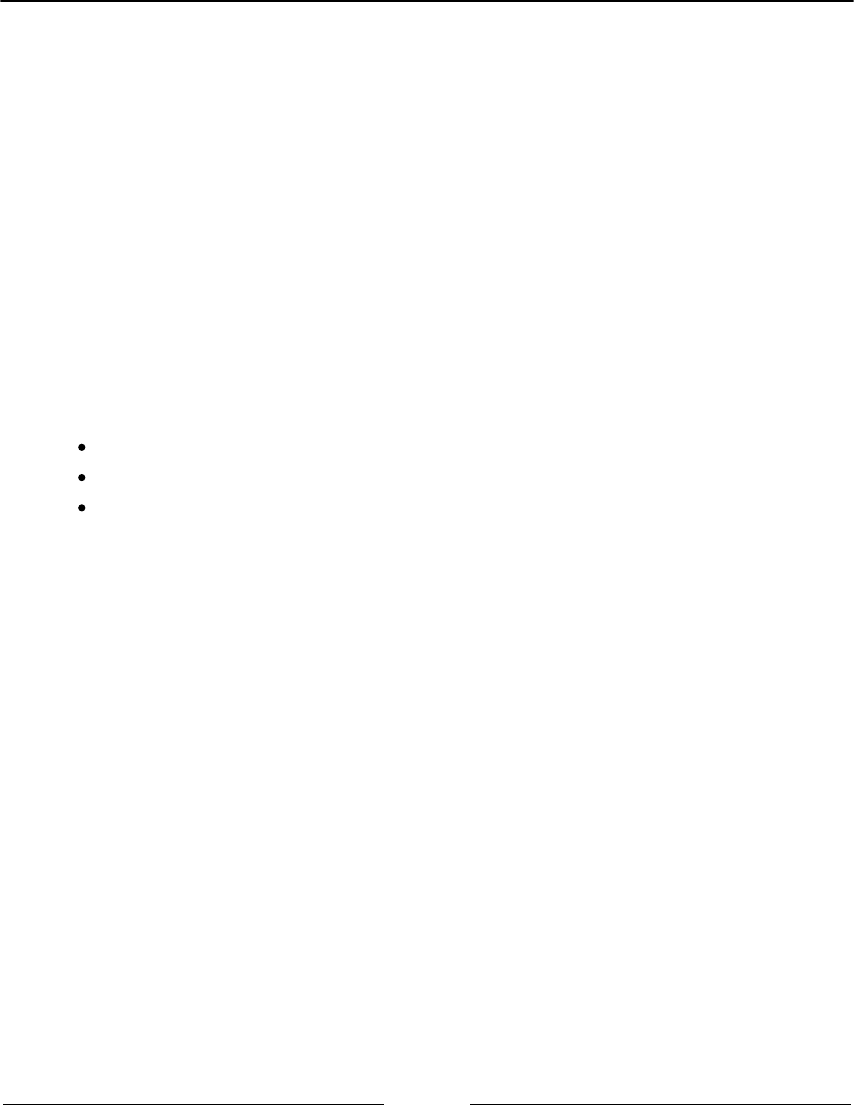
First Steps Chapter 1

[ 35 ]

Introducing Jupyter

Initially known as IPython, this project was initiated in 2001 as a free project by Fernando

Perez. By his work, the author intended to address a lack in the Python stack and provide

to the public a user programming interface for data investigations that could easily

incorporate the scientific approach (mainly meaning experimenting and interactively

discovering) in the process of data discovery and software development.

A scientific approach implies fast experimentation of different hypotheses in a reproducible

fashion (as does data exploration and analysis in data science), and when using this

interface, you will be able more naturally to implement an explorative, iterative, trial and

error research strategy during your code writing.

Recently (during Spring 2015), a large part of the IPython project was moved to a new one

called Jupyter. This new project extends the potential usability of the original IPython

interface to a wide range of programming languages, such as these:

R (https://github.com/IRkernel/IRkernel)

Julia (http://github.com/JuliaLang/IJulia.jl)

Scala (https://github.com/mattpap/IScala)

For a more complete list of available kernels for Jupyter, please

visit https://github.com/ipython/ipython/wiki/IPython-kernels-for-other-language

For instance, once having installed Jupyter and its IPython kernel, you can easily add

another useful kernel, such as the R kernel, in order to access the R language through the

same interface. All you have to do is have an R installation, run your R interface, and enter

the following commands:

install.packages(c('pbdZMQ', 'devtools'))

devtools::install_github('IRkernel/repr')

devtools::install_github('IRkernel/IRdisplay')

devtools::install_github('IRkernel/IRkernel')

IRkernel::installspec()

The commands will install the devtools library on your R, then pull and install all the

necessary libraries from GitHub (you need to be connected to the internet while running

the other commands), and finally register the R kernel both in your R installation and on

Jupyter. After that, every time you call the Jupyter Notebook, you will have the choice of

running either a Python or an R kernel, allowing you to use the same format and approach

for all your data science projects.

First Steps Chapter 1

[ 36 ]

You cannot mix the same notebook commands for different kernels; each

notebook only refers to a single kernel, that is, the one it was initially

created with.

Thanks to the powerful idea of kernels, programs that run the user's code that's

communicated by the frontend interface and provide feedback on the results of the

executed code to the interface itself, you can use the same interface and interactive

programming style no matter what language you are using for development.

In such a context, IPython is the zero kernel, the original starting one, still existing but not

intended to be used anymore to refer to the entire project.

Therefore, Jupyter can simply be described as a tool for interactive tasks that are operable

by a console or by a web-based notebook, which offers special commands that help

developers to better understand and build the code that is being currently written.

Contrary to an IDE—which is built around the idea of writing a script, running it

afterward, and finally evaluating its results—Jupyter lets you write your code in chunks,

named cells, run each of them sequentially, and evaluate the results of each one separately,

examining both textual and graphical outputs. Besides graphical integration, it provides

you with further help, thanks to customizable commands, a rich history (in the JSON

format), and computational parallelism for an enhanced performance when dealing with

heavy numeric computations.

Such an approach is also particularly fruitful for tasks involving developing code based on

data, since it automatically accomplishes the often neglected duty of documenting and

illustrating how data analysis has been done, its premises and assumptions, and its

intermediate and final results. If a part of your job is to also present your work and

persuade an internal or external stakeholder in the project, Jupyter can really do the magic

of storytelling for you with little additional effort.

You can easily combine code, comments, formulas, charts, interactive plots, and rich media

such as images and videos, making each Jupyter Notebook a complete scientific sketchpad

to find all your experimentations and their results together.

Jupyter works on your favorite browser (which could be Explorer, Firefox, or Chrome, for

instance) and, when started, presents a cell waiting for code to be written in. Each block of

code enclosed in a cell can be run, and its results are reported in the space just after the cell.

Plots can be represented in the notebook (inline plot) or in a separate window. In our

example, we decided to plot our chart inline.

First Steps Chapter 1

[ 37 ]

Moreover, written notes can be written easily using the Markdown language, a very easy

and fast-to-grasp markup language (http://daringfireball.net/projects/markdown/).

Math formulas can be handled using MathJax (https://www.mathjax.org/) to render any

LaTeX script inside HTML/markdown.

There are several ways to insert LaTeX code in a cell. The easiest way is to simply use the

Markdown syntax, wrapping the equations with a single dollar sign, $, for an inline LaTeX

formula, or with a double dollar sign, $$, for a one-line central equation. Remember that to

have a correct output, the cell should be set as Markdown. Here's an example:

In Markdown:

This is a $LaTeX$ inline equation: $x = Ax+b$

And this is a one-liner: $$x = Ax + b$$

This produces the following output:

If you're looking for something more elaborate, that is, a formula that spans for more than

one line, a table, a series of equations that should be aligned, or simply the use of special

LaTeX functions, then it's better to use the %%latex magic command offered by the Jupyter

Notebook. In this case, the cell must be in code mode and contain the magic command as

the first line. The following lines must define a complete LaTeX environment that can be

compiled by the LaTeX interpreter.

Here are a couple of examples that show you what you can do:

In:%%latex

[

|u(t)| =

begin{cases}

u(t) & text{if } t geq 0 \

-u(t) & text{otherwise }

end{cases}

]

First Steps Chapter 1

[ 38 ]

Here is the output of the first example:

In:%%latex

begin{align}

f(x) &= (a+b)^2 \

&= a^2 + (a+b) + (a+b) + b^2 \

&= a^2 + 2cdot (a+b) + b^2

end{align}

The new output when the second example is run is:

Remember that by using the %%latex magic command, the whole cell must comply with

the LaTeX syntax. Therefore, if you just need to write a few simple equations in the text, we

strongly advise that you use the Markdown method (a text-to-HTML conversion tool for

web writers developed by John Gruber, with the help of Aaron Swartz: https:/󰜌/

daringfireball.󰜌net/󰜌projects/󰜌markdown/󰜌).

Being able to integrate technical formulas in markdown is particularly fruitful for tasks

involving the development of code based on data since it automatically accomplishes the

often neglected duty of documenting and illustrating how data analysis has been managed

as well as its premises, assumptions, and intermediate and final results. If a part of your job

is to also present your work and persuade internal or external stakeholders in the project,

Jupyter can really do the magic of storytelling for you with little additional effort.

On the web page

https://github.com/ipython/ipython/wiki/A-gallery-of-interesting-IPython-Notebo

oks, there are many examples, some of which you may find inspiring for your work, as it

did for ours. Actually, we have to confess that keeping a clean, up-to-date Jupyter

Notebook has saved us uncountable times when meeting with managers and stakeholders

have suddenly popped up, requiring us to present the state of our work hastily.

First Steps Chapter 1

[ 39 ]

In short, Jupyter allows you to do the following:

See intermediate (debugging) results for each step of the analysis

Run only some sections (or cells) of the code

Store intermediate results in JSON format and have the ability to perform version

control on them

Present your work (this will be a combination of text, code, and images), share it

via the Jupyter Notebook Viewer service (http://nbviewer.jupyter.org/), and

easily export it into HTML, PDF, or even slideshows

In the next section, we will discuss Jupyter's installation in more detail and show an

example of its usage in a data science task.

Fast installation and first test usage

Jupyter is our favored choice throughout this book. It is used to clearly and effectively

illustrate and narrate operations using scripts and data, and their consequent results.

Though we strongly recommend using Jupyter, if you are using a REPL or an IDE, you can

use the same instructions and expect identical results (except for the print formats and

extensions of the returned results).

If you do not have Jupyter installed on your system, you can promptly set it up by using

the following command:

$> pip install jupyter

You can find complete instructions about Jupyter installation (covering different operating

systems) at http://jupyter.readthedocs.io/en/latest/install.html.

After installation, you can immediately start using Jupyter by calling it from the command

line:

$> jupyter notebook

Once the Jupyter instance has opened in the browser, click on the New button; in the

Notebooks section, choose Python 3 (other kernels may be present in the section depending

on what you installed).

First Steps Chapter 1

[ 40 ]

At this point, your new empty notebook will look like the following image:

At this point, you can start entering the commands in the first cell. For instance, you may

start trying typing the following into the cell where the cursor is flashing:

In: print ("This is a test")

After writing in the cell, you just press the Play button which is below the cell tab (or, as a

keyboard hotkey, you can push shift and enter buttons at the same time) to run it and

obtain an output. Then, another cell will appear for your input. As you are writing in a cell,

if you press the plus button on the menu bar, you will get a new cell, and you can move

from one cell to another using the arrows on the menu.

Most of the other functions are quite intuitive, and we invite you to try them. In order to

learn how Jupyter works, you may use a quick start guide such as

http://jupyter-notebook-beginner-guide.readthedocs.io/en/latest/, or buy a book

specializing in Jupyter functionalities.

For a complete treatise of the full range of Jupyter functionalities when

running the IPython kernel, refer to the following Packt Publishing books:

IPython Interactive Computing and Visualization Cookbook by

Cyrille Rossant, Packt Publishing, September 25, 2014

Learning IPython for Interactive Computing and Data Visualization

by Cyrille Rossant, Packt Publishing, April 25, 2013

For illustrative purposes, just consider that every Jupyter block of instructions has a

numbered input statement and an output of one. Therefore, you will find the code

presented in this book structured in two blocks, at least when the output is not trivial at all.

Otherwise, expect only the input part:

In: <the code you have to enter> Out: <the output you should get>

First Steps Chapter 1

[ 41 ]

As a rule, you just have to type the code after In: in your cells and run it. You can then

compare your output with the output that we may provide using Out:, followed by the

output that we actually obtained on our computers when we tested the code.

If you are using conda or env environments, it may happen that you

cannot find your new environments in the Jupyter interface. If that

happens, just issue conda install ipykernel from a command line

and restart the Jupyter Notebook. Your kernels should appear among the

notebook options under the New button.

Jupyter magic commands

As a special tool for interactive tasks, Jupyter offers special commands that help to better

understand the code that you are currently writing.

For instance, some of the commands are as follows:

* <object>? and <object>??: This prints a detailed description (with ??

being even more verbose) of <object>

%<function>: This uses the special <magic function>

Let's demonstrate the usage of these commands with an example. We first start the

interactive console with the jupyter command, which is used to run Jupyter from the

command line, as shown here:

$> jupyter console

Jupyter Console 4.1.1

In [1]: obj1 = range(10)

Then, in the first line of code, which is marked by Jupyter as [1], we create a list of 10

numbers (from 0 to 9), assigning the output to an object named obj1:

In [2]: obj1?

Type: range

String form: range(0, 10)

Length: 10

Docstring:

range(stop) -> range object

range(start, stop[, step]) -> range object

Return an object that produces a sequence of integers from

start (inclusive)

to stop (exclusive) by step. range(i, j) produces i, i+1, i+2,

..., j-1.

First Steps Chapter 1

[ 42 ]

start defaults to 0, and stop is omitted! range(4) produces 0,

1, 2, 3.

These are exactly the valid indices for a list of 4 elements.

When step is given, it specifies the increment (or decrement).

In [3]: %timeit x=100

The slowest run took 184.61 times longer than the fastest.

This could mean that an intermediate result is being cached.

10000000 loops, best of 3: 24.6 ns per loop

In [4]: %quickref

In the next line of code, which is numbered [2], we inspect the obj1 object using the

Jupyter command ?. Jupyter introspects the object, prints its details (obj is a range object

that can generate the values [1, 2, 3..., 9] and elements), and finally prints some

general documentation on the range objects. For complex objects, the usage of ?? instead of

? provides even more verbose output.

In line [3], we use the timeit magic function with a Python assignment (x=100). The

timeit function runs this instruction many times and stores the computational time

needed to execute it. Finally, it prints the average time that was taken to run the Python

function.

We complete the overview with a list of all the possible special Jupyter functions by

running the quickref helper function, as shown in line [4].

As you must have noticed, each time we use Jupyter, we have an input cell and, optionally,

an output cell if there is something that has to be printed on stdout. Each input is

numbered so it can be referenced inside the Jupyter environment itself. For our purposes,

we don't need to provide such references in the code of this book. Therefore, we will just

report inputs and outputs without their numbers. However, we'll use the generic In: and

Out: notations to point out the input and output cells. Just copy the commands after In: to

your own Jupyter cell and expect an output that will be reported on the following Out:.

Therefore, the basic notations will be as follows:

The In: command

The Out: output (wherever it is present and useful to be reported in this book)

Otherwise, if we expect you to operate directly on the Python console, we will use the

following form:

>>> command

First Steps Chapter 1

[ 43 ]

Wherever necessary, the command-line input and output will be written as follows:

$> command

Moreover, to run the bash command in the Jupyter console, prefix it with a ! (exclamation

mark):

In: !ls

Applications Google Drive Public Desktop

Develop

Pictures env temp

...

In: !pwd

/Users/mycomputer

Installing packages directly from Jupyter

Notebooks

Jupyter magic commands are really efficient in accomplishing different tasks, but you may

sometimes find it difficult to achieve installing new packages during a Jupyter session (and

it will happen often since you are using different environments based on conda or env). As

Jake VanderPlas explained in his blog post Installing Python Packages from a Jupyter

Notebook (https:/󰜌/󰜌jakevdp.󰜌github.󰜌io/󰜌blog/󰜌2017/󰜌12/󰜌05/󰜌installing-󰜌python-󰜌packages-

from-󰜌jupyter/󰜌), it is a matter of fact that Jupyter kernels are different from the shell you

started from, that is, you may be upgrading a wrong environment when you issue magic

commands such as !pip install numpy or !conda install --yes numpy.

Unless you are using the default Python kernel that's active on the shell on

the notebook, you actually won't succeed because your Jupyter Notebook

is pointing to a different kernel than the one operated by pip and conda

at a shell level.

The correct approach for installing, let's say, NumPy, using pip under a Jupyter Notebook

is by creating a cell like this:

In: import sys

!"{sys.executable}" -m pip install numpy

Instead, if you want to use conda, this is the cell you have to create:

In: import sys

!conda install --yes --prefix "{sys.prefix}" numpy

First Steps Chapter 1

[ 44 ]

Just replace numpy with any package you would like to install and then run, and the

installation is guaranteed to succeed.

Checking the new JupyterLab environment

If you feel like using JupyterLab and want to be a precursor of using the interface that will

become a standard in a short time, you can just switch from issuing $> jupyter

notebook to $> jupyter lab. JupyterLab will start automatically on your browser at the

http://localhost:8888 address:

You will be welcomed by a user interface composed of a launcher, where you can find

many starting options represented as icons (in the original interface they were menu items),

and a series of tabs offering direct access to files on disks, on Google Drive, showing the

running kernels and notebooks, and commands for configuring the notebook and

formatting the information in it.

Basically, it is an advanced and flexible interface, which is especially useful if you access all

such resources on a remote server, allowing you to have everything at a glance on the very

same workbench.

First Steps Chapter 1

[ 45 ]

How Jupyter Notebooks can help data scientists

The main goal of the Jupyter Notebook is easy storytelling. Storytelling is essential in data

science because you must have the power to do the following:

See intermediate (debugging) results for each step of the algorithm you're

developing

Run only some sections (or cells) of the code

Store intermediate results and have the ability to version them

Present your work (this will be a combination of text, code, and images)

Here comes Jupyter; it actually implements all of the preceding actions:

To launch the Jupyter Notebook, run the following command:1.

$> jupyter notebook

A web browser window will pop up on your desktop, backed by a Jupyter server2.

instance. This is what the main window looks like:

First Steps Chapter 1

[ 46 ]

Then, click on New Notebook. A new window will open, as shown in the3.

following screenshot. You can start using the notebook as soon as the kernel is

ready. The small circle on the top right, below the Python icon, indicates the state

of the kernel: if it's filled, it means that the kernel is busy working; if it's empty

(like the one in the screenshot), it means that the kernel is in idle, that is, ready to

run any code:

This is the web app that you'll use to compose your story. It's very similar to a Python IDE,

with the bottom section (where you can write the code) composed of cells.

A cell can be either a piece of text (eventually formatted with a markup language) or a piece

of code. In the second case, you have the ability to run the code, and any eventual output

(the standard output) will be placed under the cell. The following is a very simple example

of the same:

In: import random

a = random.randint(0, 100)

Out: 16

In: a*2

Out: 32

In the first cell, which is denoted by In:, we import the random module, assign a random

value between

and 100 to the variable a, and print the value. When this cell is run, the

output, which is denoted as Out:, is the random number. Then, in the next cell, we will just

print the double of the value of the variable a.

First Steps Chapter 1

[ 47 ]

As you can see, it's a great tool for debugging and deciding which parameter is best for a

given operation. Now, what happens if we run the code in the first cell? Will the output of

the second cell being modified since a is different? Actually, no, it won't. Each cell is

independent and autonomous. In fact, after we run the code in the first cell, we end up with

this inconsistent status:

In: import random

a = random.randint(0, 100)

Out: 56

In: a*2

Out: 32

Note that the number in the squared parentheses has changed (from 1 to

3) since it's the third executed command (and its output) from the time the

notebook started. Since each cell is autonomous, by looking at these

numbers, you can understand their order of execution.

Jupyter is a simple, flexible, and powerful tool. However, as seen in the preceding example,

you must note that when you update a variable that is going to be used later on in your

Notebook, remember to run all the cells following the updated code so that you have a

consistent state.

When you save a Jupyter Notebook, the resulting .ipynb file is JSON formatted, and it

contains all the cells and their content plus the output. This makes things easier because

you don't need to run the code to see the notebook (actually, you also don't need to have

Python and its set of toolkits installed). This is very handy, especially when you have

pictures featured in the output and some very time-consuming routines in the code. A

downside of using the Jupyter Notebook is that its file format, which is JSON structured,

cannot be easily read by humans. In fact, it contains images, code, text, and so on.

Now, let's discuss a data science-related example (don't worry about understanding it

completely):

In: %matplotlib inline

import matplotlib.pyplot as plt

from sklearn import datasets

from sklearn.feature_selection import SelectKBest, f_regression

from sklearn.linear_model import LinearRegression

from sklearn.svm import SVR

from sklearn.ensemble import RandomForestRegressor

First Steps Chapter 1

[ 48 ]

In the following cell, some Python modules are imported:

In: boston_dataset = datasets.load_boston()

X_full = boston_dataset.data

Y = boston_dataset.target

print (X_full.shape)

print (Y.shape)

Out:(506, 13)

(506,)

Then, in cell [2], the dataset is loaded and an indication of its shape is shown. The

dataset contains 506 house values that were sold in the suburbs of Boston, along with their

respective data arranged in columns. Each column of the data represents a feature. A

feature is a characteristic property of the observation. Machine learning uses features to

establish models that can turn them into predictions. If you are from a statistical

background, you can add features that can be intended as variables (values that vary with

respect to the observations).

To see a complete description of the dataset, use print boston_dataset.DESCR.

After loading the observations and their features, in order to provide a demonstration of

how Jupyter can effectively support the development of data science solutions, we will

perform some transformations and analysis on the dataset. We will use classes, such as

SelectKBest, and methods, such as .getsupport() or .fit(). Don't worry whether

these are not clear to you now; they will all be covered extensively later in this book. Try to

run the following code:

In: selector = SelectKBest(f_regression, k=1)

selector.fit(X_full, Y)

X = X_full[:, selector.get_support()]

print (X.shape)

Out:(506, 1)

For In:, we select a feature (the most discriminative one) of the SelectKBest class that is

fitted to the data by using the .fit() method. Thus, we reduce the dataset to a vector with

the help of a selection operated by indexing on all the rows and on the selected feature,

which can be retrieved by the .get_support() method.

First Steps Chapter 1

[ 49 ]

Since the target value is a vector, we can, therefore, try to see whether there is a linear

relationship between the input (the feature) and the output (the house value). When there is

a linear relationship between two variables, the output will constantly react to changes in

the input by the same proportional amount and direction:

In: def plot_scatter(X,Y,R=None):

plt.scatter(X, Y, s=32, marker='o', facecolors='white')

if R is not None:

plt.scatter(X, R, color='red', linewidth=0.5)

plt.show()

In: plot_scatter(X,Y)

The following is the output obtained after executing the preceding command:

In our example, as X increases, Y decreases. However, this does not happen at a constant

rate, because the rate of change is intense up to a certain X value, and then it decreases and

becomes constant. This is a condition of nonlinearity, and we can further visualize it using a

regression model. This model hypothesizes that the relationship between X and Y is linear

in the form of y=a+bX. Its a and b parameters are estimated according to certain criteria.

In the fourth cell, we scatter the input and output values for this problem:

In: regressor = LinearRegression(normalize=True).fit(X, Y)

plot_scatter(X, Y, regressor.predict(X))

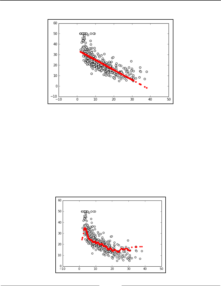
First Steps Chapter 1

[ 50 ]

The following is the output obtained after executing the preceding code:

In the next cell, we create a regressor (a simple linear regression with feature

normalization), train the regressor, and finally plot the best linear relation (that's the linear

model of the regressor) between the input and output. Clearly, the linear model is an

approximation that is not working well. We have two possible paths that we can follow at

this point. We can transform the variables in order to make their relationship linear, or we

can use a nonlinear model. Support Vector Machine (SVM) is a class of models that can

easily solve nonlinearities. Also, Random Forests is another model for automatic solving of

similar problems. Let's see them in action in Jupyter:

In: regressor = SVR().fit(X, Y)

plot_scatter(X, Y, regressor.predict(X))

The following is the output obtained after executing the preceding code:

First Steps Chapter 1

[ 51 ]

Now we proceed using the even more sophisticated algorithm, the Random Forests

regressor:

In: regressor = RandomForestRegressor().fit(X, Y)

plot_scatter(X, Y, regressor.predict(X))

The following is the output obtained after executing the preceding code:

Finally, in the last two cells, we will repeat the same procedure. This time, we will use two

nonlinear approaches: an SVM and a Random Forest-based regressor.

This demonstrative code solves the nonlinearity problem. At this point, it is very easy to

change the selected feature, regressor, and the number of features we use to train the

model, and so on by simply modifying the cells where the script is. Everything can be done

interactively, and according to the results we see, we can decide on both what should be

kept or changed and what is to be done next.

Alternatives to Jupyter

If you don't like using Jupyter, there are actually a few alternatives that can help you test

the code you will find in this book. If you have experience with R, the RStudio

(http://www.rstudio.com/) layout may appeal more to you. In this case, Yhat, a company

providing data science solutions for decision APIs, offers their data science IDE for Python

free of charge, named Rodeo (http://www.yhat.com/products/rodeo). Rodeo works by

using the IPython kernel of Jupyter under the hood, yet it is an interesting alternative given

its different user interface.

First Steps Chapter 1

[ 52 ]

The main advantages of using Rodeo are as follows:

A video layout arranged in four Windows: editor, console, plots, and

environment

Autocomplete for the editor and console

Plots are always visible inside the application in a specific Window

You can easily inspect the working variables in the environment Window

Rodeo can be simply installed using the installer. You can download it from its website, or

you can simply use the following in the command line:

$> pip install rodeo

After the installation, you can immediately run the Rodeo IDE with the following

command:

$> rodeo .

Instead, if you have experience with MATLAB from Mathworks, you will find it easier to

work with Spyder (http://pythonhosted.org/spyder/), a scientific IDE that can be found

in major Scientific Python distributions (it is present in Anaconda, WinPython, and Python

(x, y)—all distributions that we have suggested in this book). If you don't use a distribution,

in order to install Spyder, you have to follow the instructions that can be found

at http://pythonhosted.org/spyder/installation.html. Spyder allows for advanced

editing, interactive editing, debugging, and introspection features, and your scripts can be

run in a Jupyter console or in a shell-like environment.

Datasets and code used in this book

As we progress through the concepts presented in this book, in order to facilitate the

reader's understanding, learning, and memorizing processes, we will illustrate practical

and effective data science Python applications on various explicative datasets. The reader

will always be able to immediately replicate, modify, and experiment with the proposed

instructions and scripts on the data that we will use in this book.

As for the code that you are going to find in this book, we will limit our discussions to the

most essential commands in order to inspire you from the beginning of your data science

journey with Python to do more with less by leveraging key functions from the packages

we presented beforehand.

First Steps Chapter 1

[ 53 ]

Given our previous introduction, we will present the code to be run interactively as it

appears on a Jupyter console or Notebook.

All the presented code will be offered in Notebooks, which is available on the Packt website

(as pointed out in the Preface). As for the data, we will provide different examples of

datasets.

Scikit-learn toy datasets

The Scikit-learn toy dataset module is embedded in the Scikit-learn package. Such datasets

can easily be directly loaded into Python by the import command, and they don't require

any download from any external internet repository. Some examples of this type of dataset

are the Iris, Boston, and Digits datasets, to name the principal ones mentioned in

uncountable publications and books, and a few other classic ones for classification and

regression.

Structured in a dictionary-like object, besides the features and target variables, they offer

complete descriptions and contextualization of the data itself.

For instance, to load the Iris dataset, enter the following commands:

In: from sklearn import datasets

iris = datasets.load_iris()

After loading the dataset, we can explore the data description and understand how the

features and targets are stored. All Scikit-learn datasets present the following methods:

.DESCR: This provides a general description of the dataset

.data: This contains all the features

.feature_names: This reports the names of the features

.target: This contains the target values, expressed as values or numbered

classes

.target_names: This reports the names of the classes in the target

.shape: This is a method that you can apply to both .data and .target; it

reports the number of observations (the first value) and features (the second

value, if present) that are present

First Steps Chapter 1

[ 54 ]

Now, let's just try to implement them (no output is reported, but the print commands will

provide you with plenty of information):

In: print (iris.DESCR)

print (iris.data)

print (iris.data.shape)

print (iris.feature_names)

print (iris.target)

print (iris.target.shape)

print (iris.target_names)

You should know something else about the dataset—how many examples and variables are

present, and what their names are. Notice that the main data structures that are enclosed in

the iris object are the two arrays, data, and target:

In: print (type(iris.data))

Out: <class 'numpy.ndarray'>

Iris.data offers the numeric values of the variables named sepal length, sepal

width, petal length, and petal width, arranged in a matrix form (150,4), where 150 is

the number of observations and 4 is the number of features. The order of the variables is the

order presented in iris.feature_names.

Iris.target is a vector of integer values, where each number represents a distinct class

(refer to the content of target_names; each class name is related to its index number and

setosa, which is the zero element of the list, is represented as

in the target vector).

The Iris flower dataset was first used in 1936 by Ronald Fisher, who was one of the

fathers of modern statistical analysis, in order to demonstrate the functionality of linear

discriminant analysis on a small set of empirically verifiable examples (each of the 150 data

points represented iris flowers). These examples were arranged into tree-balanced species

classes (each class consisted of one-third of the examples) and were provided with four

metric descriptive variables that, when combined, were able to separate the classes.

First Steps Chapter 1

[ 55 ]

The advantage of using such a dataset is that it is very easy to load, handle, and explore for

different purposes, from supervised learning to a graphical representation. Modeling

activities take almost no time on any computer, no matter what its specifications are.

Moreover, the relationship between the classes and the role of the explicative variables are

well-known. Therefore, the task is challenging, but it is not very arduous.

For example, let's just observe how classes can be easily separated when you wish to

combine at least two of the four available variables by using a scatterplot matrix.

Scatterplot matrices are arranged in a matrix format, whose columns and rows are the

dataset variables. The elements of the matrix contain single scatterplots whose x values are

determined by the row variable of the matrix and y values by the column variable. The

diagonal elements of the matrix may contain a distribution histogram or some other

univariate representation of the variable at the same time in its row and column.

The pandas library offers an off-the-shelf function to quickly build scatterplot matrices and

start exploring relationships and distributions between the quantitative variables in a

dataset:

In: import pandas as pd

import numpy as np

colors = list()

palette = {0: "red", 1: "green", 2: "blue"}

In: for c in np.nditer(iris.target): colors.append(palette[int(c)])

# using the palette dictionary, we convert

# each numeric class into a color string

dataframe = pd.DataFrame(iris.data, columns=iris.feature_names)

In: sc = pd.scatter_matrix(dataframe, alpha=0.3, figsize=(10, 10),

diagonal='hist', color=colors, marker='o', grid=True)

First Steps Chapter 1

[ 56 ]

The following is the output obtained after executing the preceding code:

We encourage you to experiment a lot with this dataset and with similar ones before you

work on other complex real data because the advantage of focusing on an accessible, non-

trivial data problem is that it can help you to quickly build your foundations on data

science.

First Steps Chapter 1

[ 57 ]

After a while anyway, though they are useful and interesting for your learning activities,

toy datasets will start limiting the variety of different experimentations that you can

achieve. In spite of the insights provided, in order to progress, you'll need to gain access to

complex and realistic data science topics. Consequently, we will have to resort to some

external data.

The MLdata.org and other public repositories for open

source data

The second type of example dataset that we will present can be downloaded directly from

the machine learning dataset repository, or from the LIBSVM data website. Contrary to the

previous dataset, in this case, you will need access to the internet.

First, mldata.org is a public repository for machine learning datasets that is hosted by the

TU Berlin University and supported by Pattern Analysis, Statistical Modelling, and

Computational Learning (PASCAL), a network funded by the European Union. You are

free to download any dataset from this repository and experiment with it.

For example, if you need to download all the data related to earthquakes since 1972, as

reported by the United States Geological Survey, in order to analyze the data to search for

predictive patterns, you will find the data repository at

http://mldata.org/repository/data/viewslug/global-earthquakes/ (here, you will

find a detailed description of the data).

Note that the directory that contains the dataset is global-earthquakes; you can directly

obtain the data by using the following commands:

In: from sklearn.datasets import fetch_mldata

earthquakes = fetch_mldata('global-earthquakes')

print (earthquakes.data)

print (earthquakes.data.shape)

Out: (59209L, 4L)

As in the case of the Scikit-learn package toy dataset, the obtained object is a complex

dictionary-like structure, where your predictive variables are earthquakes.data and

your target to be predicted is earthquakes.target. This being the real data, in this case,

you will have quite a lot of examples and just a few variables available.

First Steps Chapter 1

[ 58 ]

LIBSVM data examples

LIBSVM Data (http://www.csie.ntu.edu.tw/~cjlin/libsvmtools/datasets/) is a page

that gathers data from many other collections. It is maintained by Chih-Jen Lin, one of the

authors of LIBSVM, a support vector machines learning algorithm for predictions (Chih-

Chung Chang and Chih-Jen Lin, LIBSVM : a library for support vector machines. ACM

Transactions on Intelligent Systems and Technology, 2:27:1--27:27, 2011). This offers different

regression, binary, and multilabel classification datasets that are stored in the LIBSVM

format. This repository is quite interesting if you wish to experiment with the support

vector machine's algorithm, and, again, it is free for you to download and use the data.

If you want to load a dataset, first go to the web page where you can visualize the data on

your browser. In the case of our example, visit

http://www.csie.ntu.edu.tw/~cjlin/libsvmtools/datasets/binary/a1a and note down

the address (a1a is a dataset that's originally from the UC Irvine Machine Learning

Repository, another open source data repository). Then, you can proceed by performing a

direct download using that address:

In: import urllib2

url =

'http://www.csie.ntu.edu.tw/~cjlin/libsvmtools/datasets/binary/a1a'

a2a = urllib2.urlopen(url)

In: from sklearn.datasets import load_svmlight_file

X_train, y_train = load_svmlight_file(a2a)

print (X_train.shape, y_train.shape)

Out: (1605, 119) (1605,)

In return, you will get two single objects: a set of training examples in a sparse matrix

format and an array of responses.

Loading data directly from CSV or text files

Sometimes, you may have to download the datasets directly from their repository by using

a web browser or a wget command (on Linux systems).

If you have already downloaded and unpacked the data (if necessary) into your working

directory, the simplest way to load your data and start working is offered by the NumPy

and the pandas library with their respective loadtxt and read_csv functions.

First Steps Chapter 1

[ 59 ]

For instance, if you intend to analyze the Boston housing data and use the version present

at http://mldata.org/repository/data/viewslug/regression-datasets-housing, you

first have to download the regression-datasets-housing.csv file in your local

directory.

You can use the following link for a direct download of the

dataset: http://mldata.org/repository/data/download/csv/regression-datasets-hous

ing.

Since the variables in the dataset are all numeric (13 continuous and one binary), the fastest

way to load and start using it is by trying out the loadtxt NumPy function and directly

loading all the data into an array.

Even in real-life datasets, you will often find mixed types of variables, which can be

addressed by pandas.read_table or pandas.read_csv. Data can then be extracted by

the values method; loadtxt can save a lot of memory if your data is already numeric. In

fact, the loadtxt command doesn't require any in-memory duplication:

In: housing = np.loadtxt('regression-datasets-housing.csv',

delimiter=',')

print (type(housing))

Out: <class 'numpy.ndarray'>

In: print (housing.shape)

Out: (506, 14)

The loadtxt function expects, by default, tabulation as a separator between the values on a

file. If the separator is a colon (,) or a semicolon(;), you have to make it explicit by using

the parameter delimiter:

>>> import numpy as np

>>> type(np.loadtxt)

>>> help(np.loadtxt)

Help on the loadtxt function can be found in

the numpy.lib.npyio module.

Another important default parameter is dtype, which is set to float.

First Steps Chapter 1

[ 60 ]

This means that loadtxt will force all of the loaded data to be converted

into a floating-point number.

If you need to determinate a different type (for example, int), you have to declare it

beforehand.

For instance, if you want to convert numeric data to int, use the following code:

In: housing_int =housing.astype(int)

Printing the first three elements of the row of the housing and housing_int arrays can

help you understand the difference:

In: print (housing[0,:3], 'n', housing_int[0,:3])

Out: [ 6.32000000e-03 1.80000000e+01 2.31000000e+00]

[ 0 18 2]

Frequently, though not always the case in our example, the data on files feature in the first

line of a textual header contains the name of the variables. In this situation, the parameter

that is skipped will point out the row in the loadtxt file from where it will start reading

the data. Being the header on row

(in Python, counting always starts from 0),

the skip=1 parameter will save the day and allow you to avoid an error and fail to load

your data.

The situation would be slightly different if you were to download the Iris dataset, which is

present at http://mldata.org/repository/data/viewslug/datasets-uci-iris/. In fact,

this dataset presents a qualitative target variable, class, which is a string that expresses the

iris species. Specifically, it's a categorical variable with four levels.

Therefore, if you were to use the loadtxt function, you will get a value error because an

array must have all its elements of the same type. The variable class is a string, whereas the

other variables are constituted by floating-point values.

The pandas library offers the solution to this and many similar cases, thanks to its

DataFrame data structure that can easily handle datasets in a matrix form (row per

columns) that is made up of different types of variables.

First, just download the datasets-uci-iris.csv file and have it saved in your local

directory.

First Steps Chapter 1

[ 61 ]

The dataset can be downloaded from

http://archive.ics.uci.edu/ml/machine-learning-databases/iris/. This archive is the

UC Irvine Machine Learning Repository, which currently maintains 440 datasets as a

service to the machine learning community. Apart from this Iris dataset, you are free to

download and try any other dataset present in the repository.

At this point, using read_csv from pandas is quite straightforward:

In: iris_filename = 'datasets-uci-iris.csv'

iris = pd.read_csv(iris_filename, sep=',', decimal='.',

header=None, names= ['sepal_length', 'sepal_width', \

'petal_length', 'petal_width', 'target'])

print (type(iris))

Out: <class 'pandas.core.frame.DataFrame'>

In order to not make the snippets of code printed in this book too cumbersome, we often

wrap it and make it nicely formatted. When necessary, in order to safely interrupt the code

and wrap it to a new line, we use the backslash symbol \ as in the preceding code example.

When rendering the code of the book by yourself, you can ignore backslash symbols and go

on writing all of the instructions on the same line, or you can digit the backslash and start a

new line continuing with the code instructions. Please be warned that typing the backslash

and then continuing the instruction on the same line will cause an execution error.

Apart from the filename, you can specify the separator (sep), the way the decimal points

are expressed (decimal), whether there is a header (in this case, header=None; normally, if

you have a header, then header=0), and the name of the variable where there is one (you

can use a list; otherwise, pandas will provide some automatic naming).

Also, we have defined names that use single words (instead of spaces, we

used underscores). Thus, we can later directly extract single variables by

calling them as we do for methods; for instance, iris.sepal_length

will extract the sepal length data.

At this point, if you need to convert the pandas DataFrame into a couple of NumPy arrays

that contain the data and target values, this can be done easily in a couple of commands:

In: iris_data = iris.values[:,:4]

iris_target, iris_target_labels = pd.factorize(iris.target)

print (iris_data.shape, iris_target.shape)

Out: (150, 4) (150,)

First Steps Chapter 1

[ 62 ]

Scikit-learn sample generators

As a last learning resource, the Scikit-learn package also offers the possibility to quickly

create synthetic datasets for regression, binary and multilabel classification, cluster analysis,

and dimensionality reduction.

The main advantage of recurring synthetic data lies in its instantaneous creation in the

working memory of your Python console. It is, therefore, possible to create bigger data

examples without having to engage in long downloading sessions from the internet (and

saving a lot of stuff on your disk).

For example, you may need to work on a classification problem involving a million data

points:

In: from sklearn import datasets

X,y = datasets.make_classification(n_samples=10**6,

n_features=10, random_state=101)

print (X.shape, y.shape)

Out: (1000000, 10) (1000000,)

After importing just the datasets module, we ask, using the make_classification

command, for one million examples (the n_samples parameter) and 10 useful features

(n_features). The random_state should be 101, so we are assured that we can replicate

the same datasets at a different time and in a different machine.

For instance, you can type the following command:

In: datasets.make_classification(1, n_features=4, random_state=101)

This will always give you the following output:

Out: (array([[-3.31994186, -2.39469384, -2.35882002, 1.40145585]]),

array([0]))

No matter what the computer and the specific situation are, random_state assures

deterministic results that make your experimentations perfectly replicable.

Defining the random_state parameter using a specific integer number (in this case, it's

101, but it may be any number that you prefer or find useful) allows easy replication of the

same dataset on your machine, the way it is set up, on different operating systems, and on

different machines.

By the way, did it take too long?

First Steps Chapter 1

[ 63 ]

On a i3-2330M CPU @ 2.20 GHz machine, it takes this:

In: %timeit X,y = datasets.make_classification(n_samples=10**6,

n_features=10, random_state=101)

Out: 1 loops, best of 3: 1.17 s per loop

If it doesn't seem like it did take too long on your machine, and if you are ready, having set

up and tested everything up to this point, we can start our data science journey.

Summary

In this introductory chapter, we installed everything that we will be using throughout this

book, from Python packages to examples. They were installed either directly or by using a

scientific distribution. We also introduced Jupyter Notebooks and demonstrated how you

can have access to the data run in the tutorials.

In the next chapter, Data Munging, we will have an overview of the data science pipeline

and explore all the key tools to handle and prepare data before you apply any learning

algorithm and set up your hypothesis experimentation schedule.

Data Munging

We are just getting into the action with data! In this chapter, you'll learn how to munge

data. What does data munging mean ?

The term mung is a technical term that was coined about half a century ago by students of

at Massachusetts Institute of Technology (MIT). Munging means to change, in a series of

well-specified and reversible steps, a piece of original data to a completely different (and

hopefully more useful) one. Deep-rooted in hacker culture, munging is often described in

the data science pipeline using other, almost synonymous, terms such as data wrangling or

data preparation.

Given such premises, in this chapter, the following topics will be covered:

The data science process (so that you'll know what is going on and what's next)

Uploading data from a file

Selecting the data you need

Cleaning up any missing or wrong data

Adding, inserting, and deleting data

Grouping and transforming data to obtain new and meaningful information

Managing to obtain a dataset matrix or an array to feed into the data science

pipeline

The data science process

Although every data science project is different, for our illustrative purposes, we can

partition an ideal data science project into a series of reduced and simplified phases.

The process starts by obtaining data (a phase known as data ingestion). Data ingestion

implies a series of possible alternatives, from simply uploading data to assembling it from

RDBMS or NoSQL repositories, or from synthetically generating it to scraping it from web

APIs or HTML pages.

Data Munging Chapter 2

[ 65 ]

Especially when faced with novel challenges, uploading data can reveal itself as a critical

part of a data scientist's work. Your data can arrive from multiple sources: databases, CSV

or Excel files, raw HTML, images, sound recordings, APIs (if you are clueless about what

an API is, you can read a good tutorial about APIs with Python here: https:/󰜌/󰜌www.

dataquest.󰜌io/󰜌blog/󰜌python-󰜌api-󰜌tutorial/󰜌) providing JavaScript Object Notation

(JSON) files, and so on. Given the wide range of alternatives, we will just briefly touch

upon this aspect by offering the basic tools to get your data (even if it is too big) into your

computer memory by using either a textual file that's present on your hard disk or the web,

or tables in a relational database management system (RDBMS).

After successfully uploading your data comes the data munging phase. Although now

available in-memory, inevitably, your data will surely be in a form that's unsuitable for any

analysis and experimentation. Data in the real world is complex, messy, and sometimes

even erroneous or missing. Yet, thanks to a bunch of basic Python data structures and

commands, you'll address all the problematic data and feed it into the next phases of the

project, appropriately transformed into a typical dataset that has observations in rows and

variables in columns. A dataset is a basic requirement for any statistical and machine

learning analysis, and you may hear it being mentioned as the flat file (when it is the result

of joining together multiple relational tables from a database) or data matrix (when

columns and rows are unlabeled and the values it contains are just numeric).

Though less rewarding than other intellectually stimulating phases (such as the application

of algorithms or machine learning), data munging creates the foundations for every

complex and sophisticated value-added analysis that you may have in mind to obtain. The

success of your project heavily relies on it.

Having completely defined the dataset that you'll be working on, a new phase opens up. At

this time, you'll start observing your data; then, you will proceed to develop and test your

hypothesis in a recurring loop. For instance, you'll explore your variables graphically. With

the help of descriptive stats, you'll figure out how to create new variables by putting your

domain knowledge into action. You'll address redundant and unexpected information

(outliers, first of all) and select the most meaningful variables and effective parameters to be

tested by a selection of machine learning algorithms.

This phase is structured as a pipeline, where your data is processed according to a series of

steps. After that, a model is finally created, but you may realize that you have to reiterate

and start again from data munging or somewhere in the data pipeline, supplying

corrections or trying different experiments, until you have reached a meaningful result.

Data Munging Chapter 2

[ 66 ]

From our experience on the field, we can assure you that no matter how promising your

plans were when starting to analyze the data, in the end, your solution will be much

different from any first envisioned idea. The confrontation with the experimental results

you will obtain rules the kind of data munging, optimizations, models, and the overall

number of iterations you have to go through before reaching a satisfactory end to your

project. That is why if you want to be a successful data scientist, it won't suffice at all just to

provide theoretically sound solutions. It is necessary to be able to quickly prototype a large

number of possible solutions in the fastest time in order to ascertain which is the best path

to take. It is our purpose to help you accelerate to the maximum by using the code snippets

provided by this book in your data science process.

A result from your project is represented by an error or optimization measure (that you

have chosen carefully in order to represent your business targets). Besides an error

measurement, your achievement can also be communicated by an interpretable insight that

has to be verbally or visually described to your data science project's sponsors or other data

scientists. At this point, being able to visualize results and insights appropriately using

tables, charts, and plots is indeed essential.

This process can also be described using the acronym OSEMN (Obtain, Scrub, Explore,

Model, iNterpret), as introduced by Hilary Mason and Chris Wiggins in a famous post on

the blog dataists (http://www.dataists.com/2010/09/a-taxonomy-of-data-science/),

describing a data science taxonomy. OSEMN is also quite memorable since it rhymes with

the words possum and awesome:

We won't ever get tired of remarking how everything starts with munging your data and

that munging can easily require up to 80% of your efforts in a data project. Since even the

longest journey starts with a single step, let's immediately step into this chapter and learn

the building blocks of a successful munging phase!

Data Munging Chapter 2

[ 67 ]

Data loading and preprocessing with pandas

In the previous chapter, we discussed where to find useful datasets and examined the basic

import commands of Python packages. In this section, having kept your toolbox ready, you

are about to learn how to structurally load, manipulate, process, and polish data using

pandas and NumPy.

Fast and easy data loading

Let's start with a CSV file and pandas. The pandas library offers the most accessible and

complete functionality to load tabular data from a file (or a URL). By default, it will store

data in a specialized pandas data structure, index each row, separate variables by custom

delimiters, infer the right data type for each column, convert data (if necessary), as well as

parse dates, missing values, and erroneous values.

We will start by importing the pandas package and reading our Iris dataset:

In: import pandas as pd

iris_filename = 'datasets-uci-iris.csv'

iris = pd.read_csv(iris_filename, sep=',', decimal='.', header=None,

names= ['sepal_length', 'sepal_width',

'petal_length', 'petal_width',

'target'])

You can specify the name of the file, the character used as a separator (sep), the character

used for the decimal placeholder (decimal), whether there is a header (header), and the

variable names (using names and a list). The settings of the sep=',' and decimal='.'

parameters have default values, and they are redundant in function. For European-style

CSV, it is important to point out both since, in many European countries, the separator

character and the decimal placeholder are different from the default ones.

If the dataset is not available online, you can follow these steps to download it from the

internet:

In: import urllib

url = "http://aima.cs.berkeley.edu/data/iris.csv"

set1 = urllib.request.Request(url)

iris_p = urllib.request.urlopen(set1)

iris_other = pd.read_csv(iris_p, sep=',', decimal='.',

header=None, names= ['sepal_length', 'sepal_width',

'petal_length', 'petal_width',

'target'])

iris_other.head()

Data Munging Chapter 2

[ 68 ]

The resulting object, named iris, is a pandas DataFrame. It's more than a simple Python

list or dictionary, and in the sections that follow, we will explore some of its features. To get

an idea of its content, you can print the first (or the last) row(s) by using the following

commands:

In: iris.head()

The head of the DataFrame will be printed in the output:

In: iris.tail()

The function, if called without arguments, will print five lines. If you want to get back a

different number of rows, just call the function using the number of rows you want to see

as an argument, as follows:

In: iris.head(2)

The preceding command will print only the first two lines. Now, to get the names of the

columns, you can simply use the following method:

In: iris.columns

Out: Index(['sepal_length', 'sepal_width',

'petal_length', 'petal_width',

'target'], dtype='object')

The resulting object is a very interesting one. It looks like a list, but it is actually a pandas

index. As suggested by the object's name, it indexes the columns' names. To extract the

target column, for example, you can simply do the following:

In: y = iris['target']

Out: 0 Iris-setosa

1 Iris-setosa

Data Munging Chapter 2

[ 69 ]

2 Iris-setosa

3 Iris-setosa

...

149 Iris-virginica

Name: target, dtype: object

The type of the object y is a pandas series. Right now, think of it as a one-dimensional array

with axis labels, as we will investigate it in depth later on. Now, we just understood that a

pandas Index class acts like a dictionary index of the table's columns. Note that you can

also get a list of columns referring to them by their indexes, as follows:

In: X = iris[['sepal_length', 'sepal_width']]

Out: [150 rows x 2 columns]

Here are the four head rows of the X dataset:

And here are the four tail ones:

Data Munging Chapter 2

[ 70 ]

In this case, the result is a pandas DataFrame. Why such a difference in results when using

the same function? In the first case, we asked for a column. Therefore, the output was a 1D

vector (that is, a pandas series). In the second example, we asked for multiple columns and

we obtained a matrix-like result (and we know that matrices are mapped as pandas

DataFrames). A novice reader can simply spot the difference by looking at the heading of

the output; if the columns are labeled, then you are dealing with a pandas DataFrame. On

the other hand, if the result is a vector and it presents no heading, then that is a pandas

series.

So far, we have learned some common steps from the data science process; after you load

the dataset, you usually separate the features and target labels.

In a classification problem, target labels are the ordinal numbers or textual strings that

indicate the class associated with every set of features.

Then, the following steps require you to get an idea of how large the problem is, and

therefore, you need to know the size of the dataset. Typically, for each observation, we

count a line, and for each feature, a column.

To obtain the dimensions of the dataset, just use the attribute shape on either a pandas

DataFrame or series, as shown in the following example:

In: print (X.shape)

Out: (150, 2)

In: print (y.shape)

Out: (150,)

The resulting object is a tuple that contains the size of the matrix/array in each dimension.

Also, note that a pandas series follow the same format (that is, a tuple with only one

element).

Data Munging Chapter 2

[ 71 ]

Dealing with problematic data

Now, you should be more confident with the basics of the process and be ready to face

datasets that are more problematic, since it is very common to have messy data in reality.

Consequently, let's see what happens if the CSV file contains a header and some missing

values and dates. For example, to make our example realistic, let's imagine the situation of a

travel agency:

According to the temperature of three popular destinations, they record whether1.

the user picks the first, second, or third destination:

Date,Temperature_city_1,Temperature_city_2,Temperature_city_3,Which

_destination

20140910,80,32,40,1

20140911,100,50,36,2

20140912,102,55,46,1

20140912,60,20,35,3

20140914,60,,32,3

20140914,,57,42,2

In this case, all the numbers are integers and the header is in the file. In our first2.

attempt to load this dataset, we can provide the following command:

In: import pandas as pd

In: fake_dataset = pd.read_csv('a_loading_example_1.csv', sep=',')

fake_dataset

The top rows of the fake_dataset are printed:

Data Munging Chapter 2

[ 72 ]

Pandas automatically gave the columns their actual name after picking them from the first

data row. We first detect a problem: all of the data, even the dates, have been parsed as

integers (or, in other cases, as strings). If the format of the dates is not very strange, you can

try the auto-detection routines that specify the column that contains the date data. In the

following example, it works well when using the following arguments:

In: fake_dataset = pd.read_csv('a_loading_example_1.csv',

parse_dates=[0])

fake_dataset

Here is the fake_dataset whose date column is now correctly interpreted by the

read_csv:

Now, in order to get rid of the missing values that are indicated by NaN, replace them with

a more meaningful number (let's say, 50 Fahrenheit). We can execute our command in the

following way:

In: fake_dataset.fillna(50)

At this point you will notice that there no more missing variables:

Data Munging Chapter 2

[ 73 ]

After that, all of the missing data has disappeared and it has been replaced by the constant

50.0. Treating missing data can also require different approaches. As an alternative to the

previous command, values can be replaced by a negative constant value to mark the fact

that they are different from others (and leave the guess for the learning algorithm):

In: fake_dataset.fillna(-1)

Note that this method only fills missing values in the view of the data

(that is, it doesn't modify the original DataFrame). In order to actually

change them, use the inplace=True argument command.

NaN values can also be replaced by the column's mean or median value as a way to

minimize the guessing error:

In: fake_dataset.fillna(fake_dataset.mean(axis=0))

The .mean method calculates the mean of the specified axis.

Please note that axis= 0 implies a calculation of means that spans the

rows; the consequently obtained means are derived from column-wise

computations. Instead, axis=1 spans columns and, therefore, row-wise

results are obtained. This works in the same way for all other methods

that require the axis parameter, both in pandas and NumPy.

The .median method is analogous to .mean, but it computes the median value, which is

useful if the mean is not a very good representation of the central value in the data, given a

too skewed distribution (for instance, when there are many extreme values in your feature).

Another possible problem when handling real-world datasets is when loading a dataset

containing errors or bad lines. In this case, the default behavior of the read_csv method is

to stop and raise an exception. A possible workaround, which is feasible when erroneous

examples are not the majority, is to ignore the lines causing exceptions. In many cases, such

a choice has the sole implication of training the machine learning algorithm without the

erroneous observations. As an example, let's say that you have a badly formatted dataset

and you want to load just all the good lines and ignore the badly formatted ones.

This is now your a_loading_example_2.csv file:

Val1,Val2,Val3

0,0,0

1,1,1

2,2,2,2

3,3,3

Data Munging Chapter 2

[ 74 ]

And here is what you can do with the error_bad_lines option:

In: bad_dataset = pd.read_csv('a_loading_example_2.csv',

error_bad_lines=False)

bad_dataset

Out: Skipping line 4: expected 3 fields, saw 4

The resulting output has the fourth line skipped because it has four values instead of three:

Dealing with big datasets

If the dataset you want to load is too big to fit in the memory, you can deal with it by using

a batch machine learning algorithm, which works with only a part of the data at once.

Using a batch approach also makes sense if you just need a sample of the data (let's say that

you want to take a peek at the data). Thanks to Python, you can actually load the data in

chunks. This operation is also called data streaming since the dataset flows into a

DataFrame or some other data structure as a continuous flow. As opposed to all the

previous cases, the dataset has been fully loaded into the memory in a standalone step.

With pandas, there are two ways to chunk and load a file. The first way is by loading the

dataset in chunks of the same size; each chunk is a piece of the dataset that contains all the

columns and a limited number of lines, no more than the number you actually have set in

the function call (the chunksize parameter). Note that the output of the read_csv

function, in this case, is not a pandas DataFrame, but an iterator-like object. In fact, to get

the results in memory, you need to iterate that object:

In: import pandas as pd

iris_chunks = pd.read_csv(iris_filename, header=None,

names=['C1', 'C2', 'C3', 'C4', 'C5'],

chunksize=10)

for chunk in iris_chunks:

print ('Shape:', chunk.shape)

print (chunk,'n')

Out: Shape: (10, 5)

Data Munging Chapter 2

[ 75 ]

C1 C2 C3 C4 C5

0 5.1 3.5 1.4 0.2 Iris-setosa

1 4.9 3.0 1.4 0.2 Iris-setosa

2 4.7 3.2 1.3 0.2 Iris-setosa

3 4.6 3.1 1.5 0.2 Iris-setosa

4 5.0 3.6 1.4 0.2 Iris-setosa

5 5.4 3.9 1.7 0.4 Iris-setosa

6 4.6 3.4 1.4 0.3 Iris-setosa

7 5.0 3.4 1.5 0.2 Iris-setosa

8 4.4 2.9 1.4 0.2 Iris-setosa

9 4.9 3.1 1.5 0.1 Iris-setosa

...

There will be 14 other pieces like these, each of them of Shape: 10, 5. The other method

to load a big dataset is by specifically asking for an iterator of it. In this case, you can

dynamically decide the length (that is, how many lines to get) you want for each piece of

the pandas DataFrame:

In: iris_iterator = pd.read_csv(iris_filename, header=None,

names=['C1', 'C2', 'C3', 'C4', 'C5'],

iterator=True)

In: print (iris_iterator.get_chunk(10).shape)

Out: (10, 5)

In: print (iris_iterator.get_chunk(20).shape)

Out: (20, 5)

In: piece = iris_iterator.get_chunk(2)

piece

The output represents just a chunk of the original dataset:

In this example, we first defined the iterator. Next, we retrieved a piece of data containing

10 lines. We then obtained 20 further rows, and finally the two rows that are printed at the

end.

Data Munging Chapter 2

[ 76 ]

Besides pandas, you can also use the CSV package, which offers two functions to iterate

small chunks of data from files: the reader and DictReader functions. Let's illustrate such

functions by importing the CSV package:

In:import csv

The reader inputs the data from disks to the Python lists. DictReader instead transforms

the data into a dictionary. Both functions work by iterating over the rows of the file being

read. The reader returns exactly what it reads, stripped of the return carriage, and splits

into a list by the separator (which is a comma by default, but this can be modified).

DictReader will map the list's data into a dictionary, whose keys will be defined by the

first row (if a header is present) or the fieldnames parameter (using a list of strings that

reports the column names).

The reading of lists in a native manner is not a limitation. For instance, it will be easier to

speed up the code using a fast Python implementation, such as PyPy. Moreover, we can

always convert lists into NumPy ndarrays (a data structure that we are going to introduce

soon). By reading the data into JSON-style dictionaries, it will be quite easy to get a

DataFrame.

Here is a simple example that uses such functionalities from the CSV package.

Let's pretend that our datasets-uci-iris.csv file, that was downloaded from

http://mldata.org/, is a huge file that we cannot fully load in the memory (actually, we

just pretend that this is the case because we remember that we saw the file at the beginning

of this chapter; it is made up of just 150 examples, and the CSV lacks a header row).

Therefore, our only choice is to load it into chunks. First, let's conduct an experiment:

In: with open(iris_filename, 'rt') as data_stream:

# 'rt' mode

for n, row in enumerate(csv.DictReader(data_stream,

fieldnames = ['sepal_length', 'sepal_width',

'petal_length', 'petal_width',

'target'],

dialect='excel')):

if n== 0:

print (n, row)

else:

break

Out: 0 OrderedDict([('sepal_length', '5.1'), ('sepal_width', '3.5'),

('petal_length', '1.4'), ('petal_width', '0.2'), ('target', 'Iris-

setosa')])

Data Munging Chapter 2

[ 77 ]

What does the preceding code accomplish? First, it opens a read-binary connection to the

file that aliases it as data_stream. Using the with command assures that the file is closed

after the commands placed in the preceding indentation are completely executed.

Then, it iterates (for...in) and it enumerates a csv.DictReader call, which wraps the

flow of the data from data_stream. Since we don't have a header row in the file,

fieldnames provides information about the fields' names. dialect just specifies that we

are calling the standard comma-separated CSV (we'll provide some hints on how to modify

this parameter later).

Inside the iteration, if the row being read is the first one, then it is printed. Otherwise, the

loop is stopped by a break command. The print command presents us with the row

number

and a dictionary. Therefore, you can recall every piece of data of the row by just

calling the keys bearing the variables' names.

Similarly, we can make the same code work for the csv.reader command, as follows:

In: with open(iris_filename, 'rt') as data_stream:

for n, row in enumerate(csv.reader(data_stream,

dialect='excel')):

if n==0:

print (row)

else:

break

Out: ['5.1', '3.5', '1.4', '0.2', 'Iris-setosa']

Here, the code is even more straightforward and the output is simpler, providing a list that

contains the row values in a sequence.

At this point, based on this second piece of code, we can create a generator callable from a

for-loop iteration. This retrieves the data on the fly from the file in the blocks of the size

defined by the batch parameter of the function:

In: def batch_read(filename, batch=5):

# open the data stream

with open(filename, 'rt') as data_stream:

# reset the batch

batch_output = list()

# iterate over the file

for n, row in enumerate(csv.reader(data_stream, dialect='excel')):

# if the batch is of the right size

if n > 0 and n % batch == 0:

# yield back the batch as an ndarray

yield(np.array(batch_output))

# reset the batch and restart

Data Munging Chapter 2

[ 78 ]

batch_output = list()

# otherwise add the row to the batch

batch_output.append(row)

# when the loop is over, yield what's left

yield(np.array(batch_output))

Similar to the previous example, the data is drawn out, thanks to the csv.reader function

wrapped by the enumerate function that accompanies the extracted list of data along with

the example number (which starts from zero). Based on the example number, a batch list is

either appended with the data list or returned to the main program using the generative

yield function. This process is repeated until the entire file is read and returned in batches:

In: import numpy as np

for batch_input in batch_read(iris_filename, batch=3):

print (batch_input)

break

Out: [['5.1' '3.5' '1.4' '0.2' 'Iris-setosa']

['4.9' '3.0' '1.4' '0.2' 'Iris-setosa']

['4.7' '3.2' '1.3' '0.2' 'Iris-setosa']]

Such a function can provide the basic functionality for learning with stochastic gradient

descent, as will be presented in Chapter 4, Machine Learning, where we will come back to

this piece of code and expand this example by introducing some more advanced examples.

Accessing other data formats

So far, we have worked on CSV files only. The pandas package offers similar functionality

(and functions) in order to load MS Excel, HDFS, SQL, JSON, HTML, and Stata datasets.

Since most of these formats are not used routinely in data science, the understanding of

how one can load and handle each of them is mostly left to you, who can refer to the

documentation available on the pandas website (http:/󰜌/󰜌pandas.󰜌pydata.󰜌org/󰜌pandas-

docs/󰜌version/󰜌0.󰜌16/󰜌io.󰜌html). Here, we will only demonstrate the essentials on how to

effectively use your disk space to store and retrieve information for machine learning

algorithms in a fast and efficient way. In such a case, you can leverage an SQLite database

(https:/󰜌/󰜌www.󰜌sqlite.󰜌org/󰜌index.󰜌html) in order to access specific subsets of information

and convert them into a pandas DataFrame. If you don't need to make particular selections

or filterings on the data, but your only problem is that reading data from a CSV file is time-

consuming and requires a lot of effort every time (for instance, setting the right variables

types and names), you can speed up saving and loading your data by using the HDF5 data

structure (https:/󰜌/󰜌support.󰜌hdfgroup.󰜌org/󰜌HDF5/󰜌whatishdf5.󰜌html).

Data Munging Chapter 2

[ 79 ]

In our first example, we are going to use SQLite and the SQL language to store away some

data and retrieve a filtered version of it. SQLite has quite a few advantages over other

databases: it is self-contained (all your data will be stored into a single file), serverless

(Python will provide the interface to store, manipulate, and access the data), and fast. After

importing the sqlite3 package (which is part of the Python stack, so there's no need to

install it anyway), you define two queries: one to drop any previous data table of the same

name, and one to create a new table that's capable of keeping the date, city, temperature,

and destination data (and you use integer, float, and varchar types, which correspond to

int, float, and str).

After opening the database (which at this point is created, if not present on disk), you

execute the two queries and then commit the changes (by committing, you actually start the

execution of all the previous database commands in a single batch: https:/󰜌/󰜌www.󰜌sqlite.

org/󰜌atomiccommit.󰜌html):

In: import sqlite3

drop_query = "DROP TABLE IF EXISTS temp_data;"

create_query = "CREATE TABLE temp_data \

(date INTEGER, city VARCHAR(80), \

temperature REAL, destination INTEGER);"

connection = sqlite3.connect("example.db")

connection.execute(drop_query)

connection.execute(create_query)

connection.commit()

At this point, the database has been created on disk with all of its data tables.

In the previous example, you created a database on disk. You can also

create it in-memory by changing the connection output to ':memory:',

as shown in this snippet of code: connection =

sqlite3.connect(':memory:') you can use ':memory:' to

create an in-memory database.

In order to insert the data into the database table, the best approach is to create a list of

tuples of values containing the rows of data you need to store. Then, an insert query will

take care of recording each data row. Please note that this time we are using the

executemany method for multiple commands (each row is inserted separately into the

table) instead of the previous command, execute:

In: data = [(20140910, "Rome", 80.0, 0),

(20140910, "Berlin", 50.0, 0),

(20140910, "Wien", 32.0, 1),

(20140911, "Paris", 65.0, 0)]

insert_query = "INSERT INTO temp_data VALUES(?, ?, ?, ?)"

Data Munging Chapter 2

[ 80 ]

connection.executemany(insert_query, data)

connection.commit()

At this point, we simply decide, by a selection query, what data, based on specific criteria,

we need to get in-memory, and we retrieve it by using the read_sql_query command:

In: selection_query = "SELECT date, city, temperature, destination \

FROM temp_data WHERE Date=20140910"

retrieved = pd.read_sql_query(selection_query, connection)

Now, all the data you need, in pandas DataFrame format, is contained in the retrieved

variable. All you need to do is to close the connection with the database:

In: connection.close()

In the following example, we will instead face the situation of a large CSV file that requires

a long amount of time for both loading and parsing its column variables. In such a case, we

will use a data format, HDF5, which is suitable for storing and retrieving DataFrames in a

fast fashion.

HDF5 is a file format that was originally developed by the National Center for

Supercomputing Applications (NCSA) to store and access large amounts of scientific data,

based on the requirements of NASA in the 1990s in order to have a portable file format for

the data produced by the Earth Observing System and other space observation systems.

HDF5 is arranged as a hierarchical data storage that allows saving multidimensional arrays

of a homogeneous type or group which are containers of arrays and other groups. As a

filesystem, it perfectly fits the DataFrame structure, and by means of automatic data

compressions, such a filesystem can make data loading much faster than simply reading a

CSV file, in case of large files.

The pandas package allows you to use the HDF5 format to store series

and DataFrame data structures. You may find it invaluable for storing

binary data as well, such a preprocessed images or video files. When you

need to access a large number of files from disk, you may experience some

latency in getting the data in-memory because the files are scattered in the

filesystem. Storing all the files into a single HDF5 file will simply solve the

problem. You can read how to use the h5py package, a Python package

providing an interface for storing and retrieving data in NumPy array

form, at https:/󰜌/󰜌www.󰜌h5py.󰜌org/󰜌 and especially at http:/󰜌/󰜌docs.󰜌h5py.

org/󰜌en/󰜌stable/󰜌, its main documentation website. You also can install

h5py by issuing the conda install h5py or pip install h5py

commands.

Data Munging Chapter 2

[ 81 ]

We will start by initializing the HDF5 file, example.h5, using the HDFStore command,

which allows for a low-level manipulation of the data file. After instantiating the file, you

can start using it as if it were a Python dictionary. In the following code snippet, you store

the Iris dataset under the dictionary key iris. After that, you simply close the HDF5 file:

In: storage = pd.HDFStore('example.h5')

storage['iris'] = iris

storage.close()

When you need to retrieve the data stored in the HDF5 file, you can reopen the file using

the HDFStore command. First, you check the available keys (as you would do in a

dictionary):

In: storage = pd.HDFStore('example.h5')

storage.keys()

Out: ['/iris']

Then, you allocate the desired values by recalling them through the corresponding key:

In: fast_iris_upload = storage['iris']

type(fast_iris_upload)

Out: pandas.core.frame.DataFrame

The data is promptly loaded, and the previous DataFrame is now available for further

processing under the variable fast_iris_upload.

Putting data together

Finally, pandas DataFrames can be created by merging series or other list-like data. Note

that scalars are transformed into lists, as follows:

In: import pandas as pd

my_own_dataset = pd.DataFrame({'Col1': range(5),

'Col2': [1.0]*5,

'Col3': 1.0,

'Col4': 'Hello World!'})

my_own_dataset

Data Munging Chapter 2

[ 82 ]

Here is the output for my_own_dataset:

It can be easily said that for each of the columns you want to be stacked together, you

provide their names (as the dictionary key) and values (as the dictionary value for that

key). As seen in the preceding example, Col2 and Col3 are created in two different ways,

but they provide the same resulting column of values. In this way, you can create a pandas

DataFrame that contains multiple types of data with a very simple function.

In this process, please ensure that you don't mix lists of different sizes; otherwise, an

exception will be raised, as shown here:

In: my_wrong_own_dataset = pd.DataFrame({'Col1': range(5),

'Col2': 'string', 'Col3': range(2)})

Out: ...

ValueError: arrays must all be same length

In order to assemble entire already existing DataFrames, you have to use a different

approach based on concatenation. The pandas package offers the concat command, which

operates on pandas data structures (Series and DataFrames) by stacking rows when

working on axis

(the default option) or stacking columns when concatenating on axis 1:

In: col5 = pd.Series([4, 3, 2, 1, 0])

col6 = pd.Series([0, 0, 1, 1, 1])

a_new_dataset = pd.concat([col5, col6], axis=1,

ignore_index = True,

keys=['Col5', 'Col6'])

my_new_dataset = pd.concat([my_own_dataset, a_new_dataset], axis=1)

my_new_dataset

Data Munging Chapter 2

[ 83 ]

The resulting dataset is a concatenation of the col5 and col6 series:

In the preceding example, we created a new DataFrame, a_new_dataset, based on two

Series. We just stacked the two series together, regardless of their indexes, because we

used the ignore_index parameter, which is set to True. If matching accordingly to the

indexes is important for your project, just don't use the ignore_index parameter (its

default value is False) and you'll have a new DataFrame based on the union of the two

indexes or on only the index elements that match as a result.

Joining two distinct datasets on the basis of a common column is achieved

in pd.concat by adding the parameter join='inner', which is

equivalent to a SQL inner join, (more on the topic about joins will be dealt

with after the following example).

Matching based on indexes could sometimes not be enough for your needs. Sometimes, you

may need to match different Series or DataFrames on specific columns or series of

columns. In that case, you need the merge method, which can be run from every

DataFrame.

In order to see the merge method in action, we will create a reference table containing some

values to be matched based on Col5:

In: key = pd.Series([1, 2, 4])

value = pd.Series(['alpha', 'beta', 'gamma'])

reference_table = pd.concat([key, value], axis=1,

ignore_index = True,

keys=['Col5', 'Col7'])

reference_table

Data Munging Chapter 2

[ 84 ]

Here is the concatenation between key and value into a DataFrame:

The merge is operated by setting the how parameter to left, thus achieving a SQL left

outer join. Apart from left, other possible settings of this parameter are as follows:

right: Equivalent to a SQL right outer join

outer: Equivalent to a SQL full outer join

inner: Equivalent to a SQL inner join (as previously mentioned)

In: my_new_dataset.merge(reference_table,

on='Col5', how='left')

The resulting DataFrame is a left outer join:

Getting back to our initial my_own_dataset, in order to check the type of data present in

each column, you can check the output of the dtypes attribute:

In: my_own_dataset.dtypes

Out: Col1 int64

Col2 float64

Col3 float64

Col4 object

dtype: object

Data Munging Chapter 2

[ 85 ]

The last method seen in this example is very handy if you wish to check whether a datum is

categorical, integer numerical, or floating point, and its precision. In fact, sometimes, it is

possible to increase the processing speed by rounding up floats to integers and casting

double-precision floats to single-precision floats, or by using only a single type of data. Let's

see how you can cast the type in the following example. This example can also be seen as a

broad example on how to reassign column data:

In: my_own_dataset['Col1'] = my_own_dataset['Col1'].astype(float)

my_own_dataset.dtypes

Out: Col1 float64

Col2 float64

Col3 float64

Col4 object

dtype: object

You can also obtain information about your DataFrame structure and data

types using the info() as shown in this example:

my_own_dataset.info().

Data preprocessing

We are now able to import datasets, even a big, problematic ones. Now, we need to learn

the basic preprocessing routines in order to make it feasible for the next data science step.

First, if you need to apply a function to a limited section of rows, you can create a mask. A

mask is a series of Boolean values (that is, True or False) that tells you whether the line is

selected or not.

For example, let's say we want to select all the lines of the Iris dataset that have a sepal

length greater than 6. We can simply do the following:

In: mask_feature = iris['sepal_length'] > 6.0

In: mask_feature

Out: 0 False

1 False

...

146 True

147 True

148 True

149 False

Data Munging Chapter 2

[ 86 ]

In the preceding simple example, we can immediately see which observations are True and

which are not (False), and which ones fit the selection query.

Now, let's check how you can use a selection mask on another example. We want to

substitute the Iris-virginica target label with the New label label. We can do this by

using the following two lines of code:

In: mask_target = iris['target'] == 'Iris-virginica'

iris.loc[mask_target, 'target'] = 'New label'

You'll see that all occurrences of Iris-virginica are now replaced by New label. The

loc() method is explained in the following code. Just think of it as a way to access the data

of the matrix with the help of row-column indexes.

To see the new list of the labels in the target column, we can use the unique() method.

This method is very handy if you want to first evaluate the dataset:

In: iris['target'].unique()

Out: array(['Iris-setosa', 'Iris-versicolor', 'New label'],

dtype=object)

If you want to see some statistics about each feature, you can group each column

accordingly; eventually, you can also apply a mask. The pandas method groupby will

produce a similar result to the GROUP BY clause in a SQL statement. The next method to

apply should be an aggregate method on one or multiple columns. For example, the

mean() pandas aggregate method is the counterpart of the AVG() SQL function to compute

the mean of the values in the group; the pandas aggregate method var() calculates the

variance; sum() the summation; count() the number of rows in the group; and so on.

Note that the result is still a pandas DataFrame, and therefore multiple operations can be

chained together.

Data Munging Chapter 2

[ 87 ]

Many common operations on variables, such as mean or sum, are

DataFrame methods that can be directly used on all the data, by columns

(using the parameter axis=0, that is, iris.sum(axis=0) or by rows

(using axis=1):

count: The count of non-null (NaN) values

median: Returns the median; that is, the 50th percentile

min: The lowest value

max: The highest value

mode: The mode, which is the most frequently occurring value

var: The variance, which measures the dispersion of the values

std: The standard deviation, which is the square root of the

variance

mad: The mean absolute deviation, which is a way to measure

the dispersion of the values robust to outliers

skew: The measure of skewness, indicative of the distribution

symmetry

kurt: The measure of kurtosis, indicative of the distribution

shape

As a next step, we can try a couple of examples with groupby in action. By grouping

observations by the target (that is, the label), we can check the difference between the

average value and the variance of the features for each group:

In: grouped_targets_mean = iris.groupby(['target']).mean()

grouped_targets_mean

The output is a grouped Iris dataset and the grouping function is the mean:

In: grouped_targets_var = iris.groupby(['target']).var()

grouped_targets_var

Data Munging Chapter 2

[ 88 ]

Now the grouping function is the variance:

As you may need multiple statistics on each variable, instead of creating multiple

aggregated datasets to be put together by concatenation, you can directly use the agg

method, and for each variable to apply specific functions. You define the variables by a

dictionary where keys are the variable labels and values are lists of functions to be applied

– to be called by a string (such as 'mean', 'std', 'min', 'max', 'sum', and 'prod') or by

a pre-defined function or even a lambda function declared on the spot:

In: funcs = {'sepal_length': ['mean','std'],

'sepal_width' : ['max', 'min'],

'petal_length': ['mean','std'],

'petal_width' : ['max', 'min']}

grouped_targets_f = iris.groupby(['target']).agg(funcs)

grouped_targets_f

Now each column has different grouping functions:

Later, if you need to sort the observations using a function, you can use the

.sort_index() method, as follows:

In: iris.sort_index(by='sepal_length').head()

Data Munging Chapter 2

[ 89 ]

As an output, you get the top rows of the dataset:

Finally, if your dataset contains a time series (for example, in the case of a numerical target)

and you need to apply a rolling operation to it (in the case of noisy data points), you can

simply do the following:

In: smooth_time_series = pd.rolling_mean(time_series, 5)

This can be performed for a rolling average of the values. Alternatively, you can give the

following command:

In: median_time_series = pd.rolling_median(time_series, 5)

Instead, this can be performed in order to obtain a rolling median of the values. In both of

these cases, the window had size 5 samples.

More generically, the apply() pandas method is able to perform any row-wise or column-

wise operation programmatically. apply() should be called directly on the DataFrame; the

first argument is the function to be applied row-wise or column-wise; the second argument

is the axis to apply it on. Note that the function can be a built-in, library-provided, lambda,

or any other user-defined function.

As an example of this powerful method, let's try to count how many non-zero elements

there are in each line. With the apply method, this is simple:

In: iris.apply(np.count_nonzero, axis=1).head()

Out: 0 5

1 5

2 5

3 5

4 5

dtype: int64

Data Munging Chapter 2

[ 90 ]

Similarly, to compute the non-zero elements feature-wise (that is, per column), you just

need to change the second argument and set it to

In: iris.apply(np.count_nonzero, axis=0)

Out: sepal_length 150

sepal_width 150

petal_length 150

petal_width 150

target 150

dtype: int64

Finally, to operate element-wise, the applymap() method should be used on the

DataFrame. In this case, just one argument should be provided: the function to apply.

For example, let's say you're interested in the length of the string representation of each cell.

To obtain that value, you should first cast each cell to a string value and then compute the

length. With applymap, this operation is very easy:

In: iris.applymap(lambda x:len(str(x))).head()

The top rows of the transformed DataFrame are:

When applying transformations to your data, you actually don't need to apply the same

function to each column. Using pandas apply methods, you can actually apply a

transformation to a single variable or to multiple ones, by modifying the same variables or

creating new ones in addition:

In: def square(x):

return x**2

original_variables = ['sepal_length', 'sepal_width',

'petal_length', 'petal_width']

squared_iris = iris[original_variables].apply(square)

Data Munging Chapter 2

[ 91 ]

One weak point of such an approach is that transformations can take a long time because

the pandas library is not leveraging the multiprocessing capabilities of recent CPU models.

Because of issues with multiprocessing in Windows when using Jupyter,

the following example can only run on Linux machines or on Windows

machines if transformed into a script, just as this Stack Overflow answer

suggests: https:/󰜌/󰜌stackoverflow.󰜌com/󰜌questions/󰜌37103243/

multiprocessing-󰜌pool-󰜌in-󰜌jupyter-󰜌notebook-󰜌works-󰜌on-󰜌linux-󰜌but-󰜌not-

windows.

In order to shorten such computation latency, you can leverage the multiprocessing

package by creating the parallel_apply function. Such a function takes a DataFrame, a

function, and the arguments of the function as input, and it creates a pool of workers (many

Python duplicates in-memory, where ideally each one is operating on a different CPU of

your system) to work in parallel and execute the required transformations:

In: import multiprocessing

def apply_df(args):

df, func, kwargs = args

return df.apply(func, **kwargs)

def parallel_apply(df, func, **kwargs):

workers = kwargs.pop('workers')

pool = multiprocessing.Pool(processes=workers)

df_split = np.array_split(df, workers)

results = pool.map(apply_df, [(ds, func, kwargs)

for ds in df_split])

pool.close()

return pd.concat(list(results))

When using this function, it is important to specify the correct number of workers

(depending on your system) and the axis the computation will take place on (since you

operate by columns, axis=1 is the usual parameter configuration you'll be using):

In: squared_iris = parallel_apply(iris[['sepal_length', 'sepal_width',

'petal_length', 'petal_width']],

func=square,

axis=1,

workers=4)

squared_iris

The Iris dataset is a tiny one, and in this case, the execution may take even longer than

simply applying a command, but on larger sets of data, the difference could be quite

notable, especially if you can count on a large number of workers.

Data Munging Chapter 2

[ 92 ]

As a tip, on an Intel i5 CPU, you can set workers=4 for optimal results,

while on Intel i7, you can set workers=8.

Data selection

The last topic on pandas that we'll focus on is data selection. Let's start with an example.

We might come across a situation where the dataset contains an index column. How do we

properly import it with pandas? And then, can we actively exploit it to make our job

simpler?

We will use a very simple dataset that contains an index column (this is just a counter and

not a feature). To make the example very generic, let's start the index from 100. So, the

index of row number

is 100:

n,val1,val2,val3

100,10,10,C

101,10,20,C

102,10,30,B

103,10,40,B

104,10,50,A

When trying to load a file the classic way, you'll find yourself in a situation where you have

got n as a feature (or a column). Nothing is practically incorrect, but an index should not be

used by mistake as a feature. Therefore, it is better to keep it separated. If instead, by

chance, it is used during the learning phase of your model, you may possibly incur a case of

leakage, which is one of the major sources of error in machine learning.

In fact, if the index is a random number, no harm will be done to your model's efficacy.

However, if the index contains progressive, temporal, or even informative elements (for

example, certain numeric ranges may be used for positive outcomes, and others for the

negative ones), you might incorporate into the model's leaked information. This will be

impossible to replicate when using your model on fresh data:

In: import pandas as pd

In: dataset = pd.read_csv('a_selection_example_1.csv')

dataset

Data Munging Chapter 2

[ 93 ]

Here is the read dataset:

Therefore, while loading such a dataset, we might want to specify that n is the index

column. Since the index n is the first column, we can give the following command:

In: dataset = pd.read_csv('a_selection_example_1.csv', index_col=0)

dataset

The read_csv function now uses the first column as the index:

Here, the dataset is loaded and the index is correct. Now, to access the value of a cell, there

are a few things we can do. Let's list them one by one:

First, you can simply specify the column and the line (by using its index) you are1.

interested in.

To extract the val3 of the fifth line (indexed with n=104), you can give the2.

following command:

In: dataset['val3'][104]

Out: 'A'

Data Munging Chapter 2

[ 94 ]

Apply this operation carefully since it's not a matrix and you might be tempted3.

to first input the row and then the column. Remember that it's actually a pandas

DataFrame, and the [] operator works first on columns and then on the element

of the resulting pandas Series.

To have something similar to the preceding method of accessing data, you can4.

use the .loc() method, which is label-based; that is, it works by the index and

column labels:

In: dataset.loc[104, 'val3']

Out: 'A'

In this case, you should first specify the index and then the columns you're interested in.

Please note that, sometimes, the index in a DataFrame can be expressed in

numbers. In such a case, it is easy to confuse it with a positional index, but

a numeric index is not necessarily ordered or continuous.

Finally, a fully-optimized function that specifies the positions (positional5.

indexing, as in a matrix) is iloc(). With it, you must specify the cell by using

the row number and column number:

In: dataset.iloc[4, 2]

Out: 'A'

The retrieval of submatrixes is a very intuitive operation; you simply need to6.

specify the lists of indexes instead of scalars:

In: dataset[['val3', 'val2']][0:2]

This command is equivalent to this:7.

In: dataset.loc[range(100, 102), ['val3', 'val2']]

And it is also equivalent to the following:8.

In: dataset.iloc[range(2), [2,1]]

Data Munging Chapter 2

[ 95 ]

In all the cases, the resulting DataFrame is as follows:

There is another method available for indexing in a pandas DataFrame:

the ix method works by a mix of label-based and positional

indexes: dataset.ix[104, 'val3']. Note that ix has to guess what

you are referring to. Therefore, if you don't want to mix labels and

positional indexes, loc and iloc are absolutely preferred in order to

create a more safe and effective approach. ix is to be deprecated in the

upcoming versions of pandas.

Working with categorical and textual data

Typically, you'll find yourself dealing with two main kinds of data: categorical and

numerical. Numerical data, such as temperature, amount of money, days of usage, or house

number, can be composed of either floating-point numbers (such as 1.0, -2.3, 99.99, and so

on) or integers (such as -3, 9, 0, 1, and so on). Each value that the data can assume has a

direct relation with others since they're comparable. In other words, you can say that a

feature with a value of 2.0 is greater (actually, it is double) than a feature that assumes a

value of 1.0. This type of data is very well-defined and comprehensible, with binary

operators such as equal to, greater than, and less than.

The other type of data you might see in your career is the categorical type. A categorical

datum expresses an attribute that cannot be measured and assumes values in a finite or

infinite set of values, often named levels. For example, the weather is a categorical feature,

since it takes values in a discrete set [sunny, cloudy, snowy, rainy, and foggy]. Other

examples are features that contain URLs, IPs, device brands, items you put in your e-

commerce cart, devices IDs, and so on. On this data, you cannot define the equal to, greater

than, and less than binary operators and therefore, you cannot rank them.

A plus point for both categorical and numerical values is Booleans. In fact, they can be seen

as categorical (presence/absence of a feature) or, on the other hand, as, the probability of a

feature having an exhibit (has displayed, has not displayed). Since many machine learning

algorithms do not allow the input to be categorical, Boolean features are often used to

encode categorical features as numerical values.

Data Munging Chapter 2

[ 96 ]

Let's continue with the example of the weather. If we want to map a feature that contains

the current weather and which takes values in the set [sunny, cloudy, snowy, rainy, and

foggy] and encodes them to binary features, we should create five True/False features,

with one for each level of the categorical feature. Now, the map is straightforward:

Categorical_feature = sunny binary_features = [1, 0, 0, 0, 0]

Categorical_feature = cloudy binary_features = [0, 1, 0, 0, 0]

Categorical_feature = snowy binary_features = [0, 0, 1, 0, 0]

Categorical_feature = rainy binary_features = [0, 0, 0, 1, 0]

Categorical_feature = foggy binary_features = [0, 0, 0, 0, 1]

Only one binary feature reveals the presence of the categorical feature; the others remain

This is called binary encoding or one hot encoding. By performing this easy step, we moved

from the categorical world to a numerical one. The price of this operation is its complexity

in terms of memory and computations; instead of a single feature, we now have five

features. Generically, instead of a single categorical feature with N possible levels, we will

create N features, each with two numerical values (1/0). This operation is named dummy

coding.

The pandas package helps us in this operation, making the mapping easy with one

command:

In: import pandas as pd

categorical_feature = pd.Series(['sunny', 'cloudy',

'snowy', 'rainy', 'foggy'])

mapping = pd.get_dummies(categorical_feature)

mapping

Here is the mapping dataset:

Data Munging Chapter 2

[ 97 ]

The output is a DataFrame that contains the categorical levels as column labels and the

respective binary features along the column. To map a categorical value to a list of

numerical ones, just use the power of pandas:

In: mapping['sunny']

Out: 0 1.0

1 0.0

2 0.0

3 0.0

4 0.0

Name: sunny, dtype: float64

In: mapping['cloudy']

Out: 0 0.0

1 1.0

2 0.0

3 0.0

4 0.0

Name: cloudy, dtype: float64

As seen in this example, sunny is mapped into the list of Boolean values [1, 0, 0, 0,

0], cloudy to [0, 1, 0, 0, 0], and so on.

The same operation can be done with another toolkit, Scikit-learn. It's somehow more

complex since you must first convert text to categorical indices, but the result is the same.

Let's take a peek at the previous example again:

In: from sklearn.preprocessing import OneHotEncoder

from sklearn.preprocessing import LabelEncoder

le = LabelEncoder()

ohe = OneHotEncoder()

levels = ['sunny', 'cloudy', 'snowy', 'rainy', 'foggy']

fit_levs = le.fit_transform(levels)

ohe.fit([[fit_levs[0]], [fit_levs[1]], [fit_levs[2]],

[fit_levs[3]], [fit_levs[4]]])

print (ohe.transform([le.transform(['sunny'])]).toarray())

print (ohe.transform([le.transform(['cloudy'])]).toarray())

Out: [[ 0. 0. 0. 0. 1.]]

[[ 1. 0. 0. 0. 0.]]

Basically, LabelEncoder maps the text to a 0-to-N integer number (note that in this case,

it's still a categorical variable since it makes no sense to rank it). Now, these five values are

mapped to five binary variables.

Data Munging Chapter 2

[ 98 ]

A special type of data – text

Let's introduce another type of data. Text data is a frequently used input for machine

learning algorithms since it contains a natural representation of data in our language. It's so

rich that it also contains the answer to what we're looking for. The most common approach

when dealing with text is to use a bag-of-words approach. According to this approach,

every word becomes a feature and the text becomes a vector that contains non-zero

elements for all the features (that is, the words) in its body. Given a text dataset, what's the

number of features? It is simple. Just extract all the unique words in it and enumerate them.

For a very rich text that uses all the English words, that number is in the 1 million range. If

you're not going to further process it (removal of any third person, abbreviations,

contractions, and acronyms), you might find yourself dealing with more than that, but

that's a very rare case. In a plain and simple approach, which is the target of this book, we

just let Python do its best.

The dataset used in this section is textual; it's the famous 20newsgroup (for more information

about this, visit http://qwone.com/~jason/20Newsgroups/). It is a collection of about

20,000 documents that belong to 20 topics of newsgroups. It's one of the most frequently

used (if not the topmost used) datasets that's presented while dealing with text

classification and clustering. To import it, we're going to use its restricted subset, which

contains all the science topics (medicine and space):

In: from sklearn.datasets import fetch_20newsgroups

categories = ['sci.med', 'sci.space']

twenty_sci_news = fetch_20newsgroups(categories=categories)

The first time you run this command, it automatically downloads the dataset and places it

in the $HOME/scikit_learn_data/20news_home/ default directory. You can query the

dataset object by asking for the location of the files, their content, and the label (that is, the

topic of the discussion where the document was posted). They're located in the

.filenames, .data, and .target attributes of the object, respectively:

In: print(twenty_sci_news.data[0])

Out: From: [email protected] ("F.Baube[tm]")

Subject: Vandalizing the sky

X-Added: Forwarded by Space Digest

Organization: [via International Space University]

Original-Sender: [email protected]

Distribution: sci

Lines: 12

From: "Phil G. Fraering" <[email protected]>

[...]

Data Munging Chapter 2

[ 99 ]

In: twenty_sci_news.filenames

Out: array([

'/Users/datascientist/scikit_learn_data/20news_home/20news-bydate-

train/sci.space/61116',

'/Users/datascientist/scikit_learn_data/20news_home/20news-

bydate-train/sci.med/58122',

'/Users/datascientist/scikit_learn_data/20news_home/20news-

bydate-train/sci.med/58903',

...,

'/Users/datascientist/scikit_learn_data/20news_home/20news-

bydate-train/sci.space/60774',

[...]

In: print (twenty_sci_news.target[0])

print (twenty_sci_news.target_names[twenty_sci_news.target[0]])

Out: 1

sci.space

The target is categorical, but it's represented as an integer (

for sci.med and 1 for

sci.space). If you want to read it, check against the index of the

twenty_sci_news.target array.

The easiest way to deal with the text is by transforming the body of the dataset into a series

of words. This means that, for each document, the number of times a specific word appears

in the body will be counted.

For example, let's make a small, easy-to-process dataset:

Document_1: We love data science

Document_2: Data science is hard

In the entire dataset, which contains Document_1 and Document_2, there are only six

different words: we, love, data, science, is, and hard. Given this array, we can associate

each document with a feature vector:

In: Feature_Document_1 = [1 1 1 1 0 0]

Feature_Document_2 = [0 0 1 1 1 1]

Note that we're discarding the positions of the words and retaining only the number of

times the word appears in the document. That's all.

Data Munging Chapter 2

[ 100 ]

In the 20newsletter database, with Python, this can be done in a simple way:

In: from sklearn.feature_extraction.text import CountVectorizer

count_vect = CountVectorizer()

word_count = count_vect.fit_transform(twenty_sci_news.data)

word_count.shape

Out: (1187, 25638)

First, we instantiate a CountVectorizer object. Then, we call the method to count the

terms in each document and produce a feature vector for each of them (fit_transform).

We then query the matrix size. Note that the output matrix is sparse because it's very

common to have only a limited selection of words for each document (since the number of

non-zero elements in each line is very low and it makes no sense to store all the redundant

zeros). Anyway, the output shape is (1187, 25638). The first value is the number of

observations in the dataset (the number of documents), while the latter is the number of

features (the number of unique words in the dataset).

After the CountVectorizer transforms, each document is associated with its feature

vector. Let's take a look at the first document:

In: print (word_count[0])

Out: (0, 10827) 2

(0, 10501) 2

(0, 17170) 1

(0, 10341) 1

(0, 4762) 2

(0, 23381) 2

(0, 22345) 1

(0, 24461) 1

(0, 23137) 7

[...]

You will notice that the output is a sparse vector where only non-zero elements are stored.

To check the direct correspondence to words, just try the following code:

In: word_list = count_vect.get_feature_names()

for n in word_count[0].indices:

print ('Word "%s" appears %i times' % (word_list[n],

word_count[0, n]))

Out: Word: from appears 2 times

Word: flb appears 2 times

Word: optiplan appears 1 times

Word: fi appears 1 times

Word: baube appears 2 times

Data Munging Chapter 2

[ 101 ]

Word: tm appears 2 times

Word: subject appears 1 times

Word: vandalizing appears 1 times

Word: the appears 7 times

[...]

So far, everything has been pretty simple, hasn't it? Let's move forward to another task of

increasing complexity and effectiveness. Counting words is good, but we can manage

more; we can compute their frequency. It's a measure that you can compare across

differently-sized datasets. It gives an idea of whether a word is a stop word (that is, a very

common word such as a, an, the, or is) or a rare, unique one. Typically, these terms are the

most important because they're able to characterize an instance and the features based on

these words, which are very discriminative in the learning process. To retrieve the

frequency of each word in each document, try the following code:

In: from sklearn.feature_extraction.text import TfidfVectorizer

tf_vect = TfidfVectorizer(use_idf=False, norm='l1')

word_freq = tf_vect.fit_transform(twenty_sci_news.data)

word_list = tf_vect.get_feature_names()

for n in word_freq[0].indices:

print ('Word "%s" has frequency %0.3f' % (word_list[n],

word_freq[0, n]))

Out: Word "from" has frequency 0.022

Word "flb" has frequency 0.022

Word "optiplan" has frequency 0.011

Word "fi" has frequency 0.011

Word "baube" has frequency 0.022

Word "tm" has frequency 0.022

Word "subject" has frequency 0.011

Word "vandalizing" has frequency 0.011

Word "the" has frequency 0.077

[...]

The sum of the frequencies is 1 (or close to 1 due to the approximation). This happens

because we chose the l1 norm. In this specific case, the word frequency is a probability

distribution function. Sometimes, it's nice to increase the difference between rare and

common words. In such cases, you can use the l2 norm to normalize the feature vector.

Data Munging Chapter 2

[ 102 ]

An even more effective way to vectorize text data is by using tf-idf. In brief, you can

multiply the term frequency of the words that compose a document by the inverse

document frequency of the word itself (that is, in the number of documents it appears in, or

in its logarithmically scaled transformation). This is very handy for highlighting words that

effectively describe each document and which are powerful discriminative elements among

the dataset:

In: from sklearn.feature_extraction.text import TfidfVectorizer

tfidf_vect = TfidfVectorizer() # Default: use_idf=True

word_tfidf = tfidf_vect.fit_transform(twenty_sci_news.data)

word_list = tfidf_vect.get_feature_names()

for n in word_tfidf[0].indices:

print ('Word "%s" has tf-idf %0.3f' % (word_list[n],

word_tfidf[0, n]))

Out: Word "fred" has tf-idf 0.089

Word "twilight" has tf-idf 0.139

Word "evening" has tf-idf 0.113

Word "in" has tf-idf 0.024

Word "presence" has tf-idf 0.119

Word "its" has tf-idf 0.061

Word "blare" has tf-idf 0.150

Word "freely" has tf-idf 0.119

Word "may" has tf-idf 0.054

Word "god" has tf-idf 0.119

Word "blessed" has tf-idf 0.150

Word "is" has tf-idf 0.026

Word "profiting" has tf-idf 0.150

[...]

In this example, the four most characterizing words of the first documents are caste,

baube, flb, and tm (they have the highest tf-idf score). This means that their term

frequency within the document is high, whereas they're pretty rare in the remaining

documents.

So far, for each word, we have generated a feature. What about taking a couple of words

together? That's exactly what happens when you consider bigrams instead of unigrams.

With bigrams (or generically, n-grams), the presence or absence of a word – as well as its

neighbors – matters (that is, the words near it and their disposition). Of course, you can mix

unigrams and n-grams and create a rich feature vector for each document. In the following

simple example, let's test how n-grams work:

In: text_1 = 'we love data science'

text_2 = 'data science is hard'

documents = [text_1, text_2]

documents

Data Munging Chapter 2

[ 103 ]

Out: ['we love data science', 'data science is hard']

In: # That is what we say above, the default one

count_vect_1_grams = CountVectorizer(ngram_range=(1, 1),

stop_words=[], min_df=1)

word_count = count_vect_1_grams.fit_transform(documents)

word_list = count_vect_1_grams.get_feature_names()

print ("Word list = ", word_list)

print ("text_1 is described with", [word_list[n] + "(" +

str(word_count[0, n]) + ")" for n in word_count[0].indices])

Out: Word list = ['data', 'hard', 'is', 'love', 'science', 'we']

text_1 is described with ['we(1)', 'love(1)', 'data(1)', 'science(1)']

In: # Now a bi-gram count vectorizer

count_vect_1_grams = CountVectorizer(ngram_range=(2, 2))

word_count = count_vect_1_grams.fit_transform(documents)

word_list = count_vect_1_grams.get_feature_names()

print ("Word list = ", word_list)

print ("text_1 is described with", [word_list[n] + "(" +

str(word_count[0, n]) + ")" for n in word_count[0].indices])

Out: Word list = ['data science', 'is hard', 'love data',

'science is', 'we love']

text_1 is described with ['we love(1)', 'love data(1)',

'data science(1)']

In: # Now a uni- and bi-gram count vectorizer

count_vect_1_grams = CountVectorizer(ngram_range=(1, 2))

word_count = count_vect_1_grams.fit_transform(documents)

word_list = count_vect_1_grams.get_feature_names()

print ("Word list = ", word_list)

print ("text_1 is described with", [word_list[n] + "(" +

str(word_count[0, n]) + ")" for n in word_count[0].indices])

Out: Word list = ['data', 'data science', 'hard', 'is', 'is hard', 'love',

'love data', 'science', 'science is', 'we', 'we love']

text_1 is described with ['we(1)', 'love(1)', 'data(1)', 'science(1)',

'we love(1)', 'love data(1)', 'data science(1)']

The preceding example very intuitively combines the first and second approach we

previously presented. In this case, we used a CountVectorizer, but this approach is very

common with a TfidfVectorizer. Note that the number of features explodes

exponentially when you use n-grams.

Data Munging Chapter 2

[ 104 ]

If you have too many features (the dictionary may be too rich, there may be too many n-

grams, or the computer may be just limited), you can use a trick that lowers the complexity

of the problem (but you should first evaluate the trade-off performance/trade-off

complexity). It's common to use the hashing trick where many words (or n-grams) are

hashed and their hashes collide (which makes a bucket of words). Buckets are sets of

semantically unrelated words but with colliding hashes. With HashingVectorizer(), as

shown in the following example, you can decide on the number of buckets of words you

want. The resulting matrix, of course, reflects your setting:

In: from sklearn.feature_extraction.text import HashingVectorizer

hash_vect = HashingVectorizer(n_features=1000)

word_hashed = hash_vect.fit_transform(twenty_sci_news.data)

word_hashed.shape

Out: (1187, 1000)

Note that you can't invert the hashing process (since it's a digest operation). Therefore, after

this transformation, you will have to work on the hashed features as they are. Hashing

presents quite a few advantages: allowing quick transformation of a bag of words into

vectors of features (hash buckets are our features, in this case), easily accommodating

never-previously-seen words among the features, and avoiding overfitting by having

unrelated words collide together in the same feature.

Scraping the web with Beautiful Soup

In the previous section, we discussed how to operate on textual data, given the fact that we

already have the dataset. What if we need to scrape the web and download it manually?

This process happens more often than you can expect, and it's a very popular topic of

interest in data science. For example:

Financial institutions scrape the web to extract fresh details and information

about the companies in their portfolio. Newspapers, social networks, blogs,

forums, and corporate websites are the ideal targets for these analyses.

Advertisement and media companies analyze sentiment and the popularity of

many pieces of the web to understand people's reactions.

Companies specialized in insight analysis and recommendation scrape the web

to understand patterns and model user behaviors.

Comparison websites use the web to compare prices, products, and services,

offering the user an updated synoptic table of the current situation.

Data Munging Chapter 2

[ 105 ]

Unfortunately, understanding websites is very hard work since each website is built and

maintained by different people, with different infrastructures, locations, languages, and

structures. The only common aspect among them is represented by the standard exposed

language, which, most of the time, is Hypertext Markup Language (HTML).

That's why the vast majority of web scrapers, available as of today, are only able to

understand and navigate HTML pages in a general-purpose way. One of the most used

web parsers is named Beautiful Soup. It's written in Python, it's open source, and it's very

stable and simple to use. Moreover, it's able to detect errors and pieces of malformed code

in the HTML page (always remember that web pages are often human-made products and

prone to errors).

A complete description of Beautiful Soup would require an entire book; here, we will see

just a few bits. First of all, Beautiful Soup is not a crawler. In order to download a web page,

we can (as an example) use the urllib library:

Let's download the code behind the William Shakespeare page on Wikipedia:1.

In: import urllib.request

url = 'https://en.wikipedia.org/wiki/William_Shakespeare'

request = urllib.request.Request(url)

response = urllib.request.urlopen(request)

It's time to instruct Beautiful Soup to read the resource and parse it using the2.

HTML parser:

In: from bs4 import BeautifulSoup

soup = BeautifulSoup(response, 'html.parser')

Now, the soup is ready and can be queried. To extract the title, we can simply3.

ask for the title attribute:

In: soup.title

Out: <title>William Shakespeare - Wikipedia,

the free encyclopedia</title>

As you can see, the whole title tag is returned, allowing for a deeper investigation of the

nested HTML structure. What if we want to know about the categories associated with the

Wikipedia page of William Shakespeare? It can be very useful to create a graph of the entry,

simply by recurrently downloading and parsing adjacent pages. We should first manually

analyze the HTML page itself to figure out what the best HTML tag containing the

information we're looking for is. Remember here the no free lunch theorem in data science:

there are no auto-discovery functions, and furthermore, things can change if Wikipedia

modifies its format.

Data Munging Chapter 2

[ 106 ]

After a manual analysis, we discover that categories are inside a div named 'mw-normal-

catlinks'; excluding the first link, all the others are okay. Now, it's time to program. Let's

put what we've observed into some code, printing for each category the title of the linked

page and the relative link to it:

In: section = soup.find_all(id='mw-normal-catlinks')[0]

for catlink in section.find_all("a")[1:]:

print(catlink.get("title"), "->", catlink.get("href"))

Out: Category:William Shakespeare -> /wiki/Category:William_Shakespeare

Category:1564 births -> /wiki/Category:1564_births

Category:1616 deaths -> /wiki/Category:1616_deaths

Category:16th-century English male actors -> /wiki/Category:16th-

century_English_male_actors

Category:English male stage actors -> /wiki/Category:

English_male_stage_actors

Category:16th-century English writers -> /wiki/Category:16th-

century_English_writers

We've used the find_all method twice to find all the HTML tags with the text contained

in the argument. In the first case, we were specifically looking for an ID; in the second case,

we were looking for all the "a" tags.

Given the output, then, and using the same code with the new URLs, it's possible to

recursively download the Wikipedia category pages, arriving at this point at the ancestor

categories.

A final note about scraping: always remember that this practice is not always allowed, and

when so, remember to tune down the rate of the download (at high rates, the website's

server may think you're doing a small-scale DoS attack and might eventually blacklist/ban

your IP address). For more information, you can read the terms and conditions of the

website, or simply contact the administrators.

Data processing with NumPy

Having introduced the essential pandas commands to upload and preprocess your data in

memory completely, in smaller batches, or even in single data rows, at this point of the data

science pipeline, you'll have to work on it in order to prepare a suitable data matrix for

your supervised and unsupervised learning procedures.

Data Munging Chapter 2

[ 107 ]

As a best practice, we advise that you divide the task between a phase of your work when

your data is still heterogeneous (a mix of numerical and symbolic values) and another

phase when it is turned into a numeric table of data. A table of data, or matrix, is arranged

in rows that represent your examples, and columns that contain the characteristic observed

values of your examples, which are your variables.

Following our advice, you have to wrangle between two key Python packages for scientific

analysis, pandas and NumPy, and their two pivotal data structures, DataFrame and

ndarray. This means that your data science pipeline will be more efficient and fast.

Since the target data structure that we want to feed into the following machine learning

phase is a matrix represented by the NumPy ndarray object, let's start from the result we

want to achieve, that is, how to generate a ndarray object.

NumPy's n-dimensional array

Python presents native data structures, such as lists and dictionaries, which you should use

to the best of your ability. Lists, for example, can store sequentially heterogeneous objects

(for instance, you can save numbers, texts, images, and sounds in the same list). On the

other hand, because being based on a lookup table (a hash table), dictionaries can recall

content. The content can be any Python object, and often it is a list of another dictionary.

Thus, dictionaries allow you to access complex, multidimensional data structures.

Anyway, lists and dictionaries have their own limitations, such as the following:

There's the problem with memory and speed. They are not really optimized for

using nearly contiguous chunks of memory, and this may become a problem

when trying to apply highly optimized algorithms or multiprocessor

computations, because memory handling may turn into a bottleneck.

They are excellent for storing data but not for operating on it. Therefore,

whatever you may want to do with your data, you have to first define custom

functions and iterate or map over the list or dictionary elements.

Iterating may often prove suboptimal when working on a large amount of data.

NumPy offers a ndarray object class (n-dimensional array) that has the following

attributes:

It is memory optimal (and, besides other aspects, configured to transmit data to

C or Fortran routines in the best-performing layout of memory blocks)

Data Munging Chapter 2

[ 108 ]

It allows for fast linear algebra computations (vectorization) and element-wise

operations (broadcasting) without any need to use iterations with for loops

Critical libraries, such as SciPy or Scikit-learn, expect arrays as an input for their

functions to operate correctly

All of this comes with some limitations. In fact, ndarray objects have the following

drawbacks:

They usually store only elements of a single, specific data type, which you can

define beforehand (but there's a way to define complex data and heterogeneous

data types, though they could be very difficult to handle for analysis purposes).

After they are initialized, their size is fixed. If you want to change their shape,

you have to create them anew.

The basics of NumPy ndarray objects

In Python, an array is a block of memory-contiguous data of a specific type with a header

that contains the indexing scheme and the data type descriptor.

Thanks to the indexing scheme, an array can represent a multidimensional data structure

where each element is indexed with a tuple of n integers, where n is the number of

dimensions. Therefore, if your array is unidimensional (that is, a vector of sequential data),

the index will start from zero (as in Python lists).

If it is bidimensional, you'll have to use two integers as an index (a tuple of coordinates of

type x,y); if there are three dimensions, the number of integers used will be three (a tuple

x,y,z), and so on.

At each indexed location, the array will contain data of the specified data type. An array

can store many numerical data types, as well as strings, and other Python objects. It is also

possible to create custom data types and therefore handle data sequences of different types,

though we advise against it and we suggest that you use the pandas DataFrame in such

cases. pandas data structures are indeed much more flexible for any intensive usage of

heterogeneous data types as necessary for a data scientist. Consequently, in this book, we

will consider only NumPy arrays of a specific, defined type, and leave pandas to deal with

heterogeneity.

Data Munging Chapter 2

[ 109 ]

Since the type (and the memory space it occupies in terms of bytes) of an array should be

defined from the beginning, the array creation procedure reserves the exact memory space

to contain all the data. The access, modification, and computation of the elements of an

array are therefore quite fast, though this also consequently implies that the array is fixed

and cannot be changed in its structure.

The Python list data structure is actually much more cumbersome and slow, being a

collection of pointers linking the list structure to the scattered memory locations containing

the data itself. Instead, as depicted in the following diagram, a NumPy ndarray is made of

just a pointer addressing a single memory location where data, arranged sequentially, is

stored. When you access the data in a NumPy ndarray, you'll actually require fewer

operations and less access to different memory parts than when using a list, hence the

major efficiency and speed when working with large amounts of data. As a drawback, data

connected to a NumPy array cannot be changed; it has to be recreated when inserting or

removing data:

No matter the dimensions of the NumPy array, data will always be arranged as a

continuous sequence of values (a contiguous block of memory). It is the knowledge of the

size of the array and of the strides (telling us how many bytes we have to skip in memory

to move to the next position along a certain axis) that renders it easy to correctly represent

and operate on the array.

Data Munging Chapter 2

[ 110 ]

Talking of memory optimization for fast performances, in order to store

multidimensional arrays, there are strictly two methods called row-major

order and column-major order. Since RAM (random access memory) is

arranged into a linear storage of memory cells (memory cells are

contiguous as the points of a line – there is no such thing as an array in

RAM), you have to flatten the array to a vector and store it in memory.

When flattening, you can just proceed row by row (row-major order),

which is typical of C/C++, or column by column (column-major order),

which is typical of Fortran or R. Python, in the NumPy package

implementation, uses the row-major ordering (also called C-contiguous,

whereas the column-major ordering is also called Fortran-contiguous),

which means that it is faster in computing operations applied row by row

than working column after column. Anyway, when creating your NumPy

array, you can decide the ordering of your data structure, based on your

expectation of manipulating it more by rows or columns. After importing

the package, import numpy as np, given an array such as a =

[[1,2,3],[4,5,6],[7,8,9]], you can redefine it in row-major order: c

= np.array(a, order='C') or in column-major order: f =

np.array(a, order='F')

In contrast, lists of data structures, that represent multiple dimensions, cannot but turn

themselves into nested lists, thus increasing both overhead and memory fragmentation

when accessing data.

All that you have read so far may sound like a computer scientist

blabbering. After all, all data scientists care about is getting Python to do

something useful and quick. That's surely true, but doing something

quickly from a syntactic point of view sometimes doesn't automatically

equate into doing something quick from the point of view of the execution

itself. If you can grasp the internals of NumPy and pandas, you could

really make your code speed up and achieve more in your projects in less

time. We have experience of syntactically correct data munging code

using NumPy and pandas that, by the right refactoring, reduced its

execution time by half or more.

Data Munging Chapter 2

[ 111 ]

For our purposes, it is also very important to understand that, when accessing or

transforming an array, we may be just viewing it or we may be copying it. When we are

viewing an array, we actually call a procedure that allows us to convert the data that's

present in its structure into something else, but the sourcing array is unaltered. Based on

the previous example, when viewing, we are just changing the size attribute of a ndarray;

the data is left untouched. Consequently, any data transformation experienced as viewing

an array is merely ephemeral, unless we fix them into a new array.

Instead, when we are copying an array, we are effectively creating a new array with a

different structure (thus occupying fresh memory). We do not just change the parameter

relative to the size of the array; we are also reserving another sequential chunk of memory

and copying our data there.

All pandas DataFrames are actually made of one-dimensional NumPy

arrays. For this reason, they inherit the speed and memory efficiency of

ndarrays when you operate by columns (since each column is a NumPy

array). When operating by rows, DataFrames are more inefficient because

you are accessing sequentially different columns; that is, different NumPy

arrays. For the same reason, it is speedier to address portions of a pandas

DataFrame by a positional index, not by a pandas index, because NumPy

arrays work using integer numbers as positions. Using pandas indexes

(which can also be textual, not just numerical) actually requires a

transformation of the index into its corresponding position for the

DataFrame to operate correctly on the data.

Creating NumPy arrays

There is more than one way to create NumPy arrays. The following are some of the ways

you can create them:

By transforming an existing data structure into an array

By creating an array from scratch and populating it with default or calculated

values

By uploading some data from a disk into an array

If you are going to transform an existing data structure, the odds are in favor of you

working with a structured list or a pandas DataFrame.

Data Munging Chapter 2

[ 112 ]

From lists to unidimensional arrays

One of the most common situations you will encounter when working with data is

transforming a list into an array.

When operating such a transformation, it is important to consider the objects the lists

contain because this will determine the dimensionality and the dtype of the resulting

array.

Let's start with this first example of a list containing just integers:

In: import numpy as np

In: # Transform a list into a uni-dimensional array

list_of_ints = [1,2,3]

Array_1 = np.array(list_of_ints)

In: Array_1

Out: array([1, 2, 3])

Remember that you can access a one-dimensional array as you would with a standard

Python list (the indexing starts from zero):

In: Array_1[1] # let's output the second value

Out: 2

We can ask for further information about the type of the object and the type of its elements

(the effectively resulting type depends on whether your system is 32-bit or 64-bit):

In: type(Array_1)

Out: numpy.ndarray

In: Array_1.dtype

Out: dtype('int64')

The default dtype depends on the system you're operating on.

Data Munging Chapter 2

[ 113 ]

Our simple list of integers will turn into a one-dimensional array; that is, a vector of 32-bit

integers (ranging from -231 to 231-1, the default integer on the platform we used for our

examples).

Controlling memory size

You may think that it is a waste of memory to use an int64 data type if the range of your

values is so limited.

In fact, conscious of data-intensive situations, you can calculate how much memory space

your Array_1 object is taking:

In: import numpy as np

Array_1.nbytes

Out: 24

Please note that on 32-bit platforms (or when using a 32-bit Python

version on a 64-bit platform), the result is 12.

In order to save memory, you can specify the type that best suits your array beforehand:

In: Array_1 = np.array(list_of_ints, dtype= 'int8')

Now, your simple array occupies just a fourth of the previous memory space. It may seem

an obvious and overly simplistic example, but when dealing with millions of rows and

columns, defining the best data type for your analysis can really save the day, allowing you

to fit everything nicely into memory.

For your reference, here is a table that presents the most common data types for data

science applications and their memory usage for a single element:

Type Size in bytes Description

bool

Boolean (True or False) stored as a byte

int

Default integer type (normally int32 or int64)

int8

1 Byte (-128 to 127)

int16

2 Integer (-32768 to 32767)

int32

4 Integer (-2**31 to 2**31-1)

int64

8 Integer (-2**63 to 2**63-1)

Data Munging Chapter 2

[ 114 ]

Type Size in bytes Description

uint8

1 Unsigned integer (0 to 255)

uint16

2 Unsigned integer (0 to 65535)

uint32

4 Unsigned integer (0 to 2**32-1)

uint64

8 Unsigned integer (0 to 2**64-1)

float_

Shorthand for float64

float16

2 Half-precision float (exponent 5 bits, mantissa 10 bits)

float32

4 Single-precision float (exponent 8 bits, mantissa 23 bits)

float64

8 Double-precision float (exponent 11 bits, mantissa 52 bits)

There are some more numerical types, such as complex numbers, that are

less usual but which may be required by your application (for example, in

a spectrogram). You can get the complete idea from the NumPy user

guide at http://docs.scipy.org/doc/numpy/user/basics.types.html.

If an array has a type that you want to change, you can easily create a new array by casting

a new, specified type:

In: Array_1b = Array_1.astype('float32')

Array_1b

Out: array([ 1., 2., 3.], dtype=float32)

In case your array is memory consuming, note that the .astype method will copy the

array, and thus it always creates a new array.

Heterogeneous lists

What if the lists were made of heterogeneous elements, such as integers, floats, and strings?

This gets trickier. A quick example can describe the situation to you:

In: import numpy as np

complex_list = [1,2,3] + [1.,2.,3.] + ['a','b','c']

# at first the input list is just ints

Array_2 = np.array(complex_list[:3])

print ('complex_list[:3]', Array_2.dtype)

# then it is ints and floats

Array_2 = np.array(complex_list[:6])

print ('complex_list[:6]', Array_2.dtype)

# finally we add strings print

Array_2 = np.array(complex_list)

('complex_list[:] ',Array_2.dtype)

Data Munging Chapter 2

[ 115 ]

Out: complex_list[:3] int64

complex_list[:6] float64

complex_list[:] <U32

As explicated by our output, it seems that float types prevail over int types, and strings

(<U32 means a Unicode string of size 32 or less) take over everything else.

While creating an array using lists, you can mix different elements, and the most Pythonic

way to check the results is by questioning the dtype of the resulting array.

Be aware that if you are uncertain about the contents of your array, you really have to

check. Otherwise, you may find it impossible to operate on your resulting array and you

may incur in an error later (unsupported operand type):

In: # Check if a NumPy array is of the desired numeric type

print (isinstance(Array_2[0],np.number))

Out: False

In our data munging process, unintentionally finding out an array of the string type as

output would mean that we forgot to transform all variables into numeric ones in the

previous steps; for example, when all the data was stored in a pandas DataFrame. In the

previous section, Working with categorical and textual data, we provided some simple and

straightforward ways to deal with such situations.

Before that, let's complete our overview of how to derive an array from a list object. As we

mentioned previously, the type of objects in the list influences the dimensionality of the

array, too.

From lists to multidimensional arrays

If a list containing numeric or textual objects is rendered into a unidimensional array (that

could represent a coefficient vector, for instance), a list of lists translates into a two-

dimensional array, and a list of list of lists becomes a three-dimensional one:

In: import numpy as np

# Transform a list into a bidimensional array

a_list_of_lists = [[1,2,3],[4,5,6],[7,8,9]]

Array_2D = np.array(a_list_of_lists )

Array_2D

Out: array([[1, 2, 3],

[4, 5, 6],

[7, 8, 9]])

Data Munging Chapter 2

[ 116 ]

As mentioned previously, you can call out single values with indices, as in a list, though

here you'll have two indices—one for the row dimension (also called axis 0) and one for the

column dimension (axis 1):

In: Array_2D[1, 1]

Out: 5

Two-dimensional arrays are usually the norm in data science problems, though three-

dimensional arrays may be found when a dimension represents time, for instance:

In: # Transform a list into a multi-dimensional array

a_list_of_lists_of_lists = [[[1,2],[3,4],[5,6]],

[[7,8],[9,10],[11,12]]]

Array_3D = np.array(a_list_of_lists_of_lists)

Array_3D

Out: array([[[ 1, 2],

[ 3, 4],

[ 5, 6]],

[[ 7, 8],

[ 9, 10],

[11, 12]]])

To access single elements of a three-dimensional array, you just have to point out three

indexes:

In: Array_3D[0,2,0] # Accessing the 5th element

Out: 5

Arrays can be made from tuples in a way that is similar to the method of creating lists.

Also, dictionaries can be turned into two-dimensional arrays thanks to the .items()

method, which returns a copy of the dictionary's list of key-value pairs:

In: np.array({1:2,3:4,5:6}.items())

Out: array([[1, 2],

[3, 4],

[5, 6]])

Data Munging Chapter 2

[ 117 ]

Resizing arrays

Earlier, we mentioned how you can change the type of the elements of an array. We will

now shortly stop for a while to examine the most common instructions to modify the shape

of an existing array.

Let's start with an example that uses the .reshape method, which accepts an n-tuple

containing the size of the new dimensions as a parameter:

In: import numpy as np

# Restructuring a NumPy array shape

original_array = np.array([1, 2, 3, 4, 5, 6, 7, 8])

Array_a = original_array.reshape(4,2)

Array_b = original_array.reshape(4,2).copy()

Array_c = original_array.reshape(2,2,2)

# Attention because reshape creates just views, not copies

original_array[0] = -1

Our original array is a unidimensional vector of integer numbers from 1 to 8. Here is what

we execute in the code:

We assign Array_a to a reshaped original_array of size 4 x 21.

We do the same with Array_b, though we append the .copy() method, which2.

will copy the array into a new one

Finally, we assign Array_c to a reshaped array in three dimensions of size 2 x 2 x3.

After having done such an assignment, the first element of original_array is4.

changed in value from 1 to -1

Now, if we check the content of our arrays, we will notice that Array_a and Array_c,

though they have the desired shape, are characterized by -1 as the first element. That's

because they dynamically mirror the original array they are in view from:

In: Array_a

Out: array([[-1, 2],

[3, 4],

[5, 6],

[7, 8]])

In: Array_c

Out: array([[[-1, 2],

[3, 4]],

Data Munging Chapter 2

[ 118 ]

[[5, 6],

[7, 8]]])

Only the Array_b array, having been copied before mutating the original array, has a first

element with a value of 1:

In: Array_b

Out: array([[1, 2],

[3, 4],

[5, 6],

[7, 8]])

If it is necessary to change the shape of the original array, then the resize method is to be

favored:

In: original_array.resize(4,2)

original_array

Out: array([[-1, 2],

[ 3, 4],

[ 5, 6],

[ 7, 8]])

The same results may be obtained by acting on the .shape value by assigning a tuple of

values representing the size of the intended dimensions:

In: original_array.shape = (4,2)

Instead, if your array is two-dimensional and you need to exchange the rows with the

columns, that is, to transpose the array, the .T or .transpose() methods will help you

obtain such a kind of transformation (which is a view, like .reshape):

In: original_array

Out: array([[-1, 2],

[ 3, 4],

[ 5, 6],

[ 7, 8]])

Arrays derived from NumPy functions

If you need a vector or a matrix characterized by a particular numeric series (zeros, ones,

ordinal numbers, and particular statistical distributions), NumPy functions provide you

with quite a large range of choices.

Data Munging Chapter 2

[ 119 ]

First, creating a NumPy array of ordinal values (integers) is straightforward if you use the

arange function, which returns integer values in a given interval (usually from zero) and

reshapes its results:

In: import numpy as np

In: ordinal_values = np.arange(9).reshape(3,3)

ordinal_values

Out: array([[0, 1, 2],

[3, 4, 5],

[6, 7, 8]])

If the array has to be reversed in the order of values, use the following command:

In: np.arange(9)[::-1]

Out: array([8, 7, 6, 5, 4, 3, 2, 1, 0])

If the integers are just random (with no order and possibly repeated), provide the following

command:

In: np.random.randint(low=1,high=10,size=(3,3)).reshape(3,3)

Other useful arrays are either made of just zeros and ones or are identity matrices:

In: np.zeros((3,3))

In: np.ones((3,3))

In: np.eye(3)

If the array will be used for a grid search to search for optimal parameters, fractional values

in an interval or a logarithmic growth should prove most useful:

In: fractions = np.linspace(start=0, stop=1, num=10)

growth = np.logspace(start=0, stop=1, num=10, base=10.0)

Instead, statistical distributions, such as normal or uniform, may be handy for the

initialization of a vector or matrix of coefficients.

A 3 x 3 matrix of standardized normal values (mean=0, std=1) can be seen here:

In: std_gaussian = np.random.normal(size=(3,3))

Data Munging Chapter 2

[ 120 ]

If you need to specify a different mean and standard deviation, just give the following

command:

In: gaussian = np.random.normal(loc=1.0, scale= 3.0, size=(3,3))

The loc parameter stands for the mean, and the scale is actually the standard deviation.

Another frequent choice for a statistical distribution that is used to initialize a vector is

certainly the uniform distribution:

In: rand = np.random.uniform(low=0.0, high=1.0, size=(3,3))

Getting an array directly from a file

NumPy arrays can also be created directly from the data present in a file.

Let's use an example from the previous chapter:

In: import numpy as np

housing = np.loadtxt('regression-datasets-housing.csv',

delimiter=',', dtype=float)

NumPy loadtxt, given a filename, delimiter, and dtype, will upload the data to an

array, unless the dtype is wrong; for instance, there's a string variable and the required

array type is a float, as shown in the following example:

In: np.loadtxt('datasets-uci-iris.csv',delimiter=',',dtype=float)

Out: ValueError: could not convert string to float: Iris-setosa

In this case, a feasible solution could be to be aware of what column is a string (or any other

non-numeric format) and prepare a converter function to turn it into numeric thanks to

the converters parameter of loadtxt, which allows you to apply specific transformation

functions to specific columns of the array, such as in the following example:

In: def from_txt_to_iris_class(x):

if x==b'Iris-setosa': return 0

elif x==b'Iris-versicolor': return 1

elif x== b'Iris-virginica': return 2

else: return np.nan

np.loadtxt('datasets-uci-iris.csv', delimiter=',',

converters= {4: from_txt_to_iris_class})

Data Munging Chapter 2

[ 121 ]

Extracting data from pandas

Interacting with pandas is quite easy. In fact, with pandas being built upon NumPy, arrays

can easily be extracted from DataFrame objects, and they can be transformed into

DataFrames themselves.

First, let's upload some data into a DataFrame. The BostonHouse example we downloaded

in the previous chapter from the ML repository is suitable:

In: import pandas as pd

import numpy as np

housing_filename = 'regression-datasets-housing.csv'

housing = pd.read_csv(housing_filename, header=None)

As demonstrated in the Heterogeneous lists section, at this point, the .values method will

extract an array of a type that accommodates all the different types that are present in the

DataFrame:

In: housing_array = housing.values

housing_array.dtype

Out: dtype('float64')

In such a case, the selected type is float64 because the float type prevails over the int

type:

In: housing.dtypes

Out: 0 float64

1 int64

2 float64

3 int64

4 float64

5 float64

6 float64

7 float64

8 int64

9 int64

10 int64

11 float64

12 float64

13 float64

dtype: object

Data Munging Chapter 2

[ 122 ]

Asking for the types used by the DataFrame object before extracting your NumPy array by

using the .dtypes method on the DataFrame allows you to anticipate the dtype of the

resulting array. Consequently, it allows you to decide whether to transform or change the

type of the variables in the DataFrame object before proceeding (please consult

the Working with categorical and textual data section of this chapter).

NumPy fast operation and computations

When arrays need to be manipulated by mathematical operations, you just need to apply

the operation on the array with respect to a numerical constant (a scalar), or an array of the

same shape:

In: import numpy as np

a = np.arange(5).reshape(1,5)

a += 1

a*a

Out: array([[ 1, 4, 9, 16, 25]])

As a result, the operation is to be performed element-wise; that is, every element of the

array is operated by either the scalar value or the corresponding element of the other array.

When operating on arrays of different dimensions, it is still possible to obtain element-wise

operations without having to restructure the data if one of the corresponding dimensions is

1. In fact, in such a case, the dimension of size 1 is stretched until it matches the dimension

of the corresponding array. This conversion is called broadcasting.

For instance:

In: a = np.arange(5).reshape(1,5) + 1

b = np.arange(5).reshape(5,1) + 1

a * b

Out: array([[ 1, 2, 3, 4, 5],

[ 2, 4, 6, 8, 10],

[ 3, 6, 9, 12, 15],

[ 4, 8, 12, 16, 20],

[ 5, 10, 15, 20, 25]])

The preceding code is equivalent to the following:

In: a2 = np.array([1,2,3,4,5] * 5).reshape(5,5)

b2 = a2.T

a2 * b2

Data Munging Chapter 2

[ 123 ]

However, it won't require an expansion of memory of the original arrays in order to obtain

pair-wise multiplication.

Furthermore, there exists a wide range of NumPy functions that can operate element-wise

on arrays: abs(), sign(), round(), floor(), sqrt(), log(), and exp().

Other usual operations that could be operated by NumPy functions are sum() and prod(),

which provide the summation and product of the array rows or columns on the basis of the

specified axis:

In: print (a2)

Out: [[1 2 3 4 5]

[1 2 3 4 5]

[1 2 3 4 5]]

In: np.sum(a2, axis=0)

Out: array([ 5, 10, 15, 20, 25])

In: np.sum(a2, axis=1)

Out: array([15, 15, 15, 15, 15])

When operating on your data, remember that operations and NumPy functions on arrays

are extremely fast when compared to simple Python lists. Let's try out a couple of

experiments. First, let's try to compare a list comprehension to an array when dealing with

a sum of a constant:

In: %timeit -n 1 -r 3 [i+1.0 for i in range(10**6)]

%timeit -n 1 -r 3 np.arange(10**6)+1.0

Out: 1 loops, best of 3: 158 ms per loop

1 loops, best of 3: 6.64 ms per loop

On Jupyter, %time allows you to easily benchmark operations. Then, the -n 1 parameter

just requires the benchmark to execute the code snippet for only one loop; -r 3 requires

you to retry the execution of the loops (in this case, just one loop) three times and report the

best performance recorded from such repetitions.

Data Munging Chapter 2

[ 124 ]

Results on your computer may vary depending on your configuration and operating

system. Anyway, the difference between the standard Python operations and the NumPy

ones will remain quite large. Though unnoticeable when working on small datasets, this

difference can really impact your analysis when dealing with larger data or when looping

over and over the same analysis pipeline for parameter or variable selection.

This also happens when applying sophisticated operations, such as finding a square root:

In: import math

%timeit -n 1 -r 3 [math.sqrt(i) for i in range(10**6)]

Out: 1 loops, best of 3: 222 ms per loop

In: %timeit -n 1 -r 3 np.sqrt(np.arange(10**6))

Out: 1 loops, best of 3: 6.9 ms per loop

Sometimes, you may need to apply custom functions to your array instead.

The apply_along_axis function lets you use a custom function and apply it on an axis of

an array:

In: def cube_power_square_root(x):

return np.sqrt(np.power(x, 3))

np.apply_along_axis(cube_power_square_root,

axis=0, arr=a2)

Out: array([[ 1., 2.82842712, 5.19615242, 8., 11.18033989],

[ 1., 2.82842712, 5.19615242, 8., 11.18033989],

[ 1., 2.82842712, 5.19615242, 8., 11.18033989]])

Matrix operations

Apart from element-wise calculations using the np.dot() function, you can also apply

multiplications to your two-dimensional arrays based on matrix calculations, such as

vector-matrix and matrix-matrix multiplications:

In: import numpy as np

M = np.arange(5*5, dtype=float).reshape(5,5)

Out: array([[ 0., 1., 2., 3., 4.],

[ 5., 6., 7., 8., 9.],

Data Munging Chapter 2

[ 125 ]

[ 10., 11., 12., 13., 14.],

[ 15., 16., 17., 18., 19.],

[ 20., 21., 22., 23., 24.]])

As an example, we will create a 5 x 5 two-dimensional array of ordinal numbers from 0 to

24:

We will define a vector of coefficients and an array column stacking the vector1.

and its reverse:

In: coefs = np.array([1., 0.5, 0.5, 0.5, 0.5])

coefs_matrix = np.column_stack((coefs,coefs[::-1]))

print (coefs_matrix)

Out: [[ 1. 0.5]

[ 0.5 0.5]

[ 0.5 1. ]]

We can now multiply the array with the vector by using the np.dot function:2.

In: np.dot(M,coefs)

Out: array([ 5., 20., 35., 50., 65.])

Or the vector by the array:3.

In: np.dot(coefs,M)

Out: array([ 25., 28., 31., 34., 37.])

Or the array by the stacked coefficient vectors (which is a 5 x 2 matrix):4.

In: np.dot(M,coefs_matrix)

Out: array([[ 5., 7.],

[ 20., 22.],

[ 35., 37.],

[ 50., 52.],

[ 65., 67.]])

NumPy also offers an object class, matrix, which is actually a subclass of ndarray,

inheriting all its attributes and methods. NumPy matrices are exclusively two-dimensional

(as arrays are actually multi-dimensional) by default. When multiplied, they apply matrix

products, not element-wise ones (the same happens when raising powers), and they have

some special matrix methods (.H for the conjugate transpose and .I for the inverse).

Data Munging Chapter 2

[ 126 ]

Apart from the convenience of operating in a fashion that is similar to that of MATLAB,

they do not offer any other advantage. You may risk confusion in your scripts since you'll

have to handle different product notations for matrix objects and arrays.

Since Python 3.5, a new operator, the @ (at) operator, dedicated to matrix

multiplication, has been introduced in Python (the change is for all the

packages in Python, not just NumPy). The introduction of this new

operator brings a couple of advantages.

First, there won't be any more cases where the * operator will be meant to

be used for matrix multiplication. The * operator will be used exclusively

for element-wise operations (those operations where, having two matrices

(or vectors) of the same dimension, you apply the operation between the

elements having the same position in the two matrices).

Then, code that is representing formulas will gain in readability, thus

becoming much easier to read and interpret. You won't have to evaluate

operators (+ - / *) and methods (.dot) together anymore, only operators (+ -

/ * @).

You can learn more about this introduction (which is just formal –

everything you could apply before using the .dot method works with the

@ operator) and look at some examples of applications by reading the

Python Enhancement Proposal (PEP) 465 at the Python foundation

website: https://www.python.org/dev/peps/pep-0465/.

Slicing and indexing with NumPy arrays

Indexing allows us to take a view of a ndarray by pointing out either what slice of

columns and rows to visualize, or an index:

Let's define a working array:1.

In: import numpy as np

M = np.arange(10*10, dtype=int).reshape(10,10)

Our array is a 10 x 10 two-dimensional array. We can initially start by slicing it2.

into a single dimension. The notation for a single dimension is the same as that in

Python lists:

[start_index_included:end_index_exclude:steps]

Data Munging Chapter 2

[ 127 ]

Let's say that we want to extract even rows from 2 to 8:3.

In: M[2:9:2,:]

Out: array([[20, 21, 22, 23, 24, 25, 26, 27, 28, 29],

[40, 41, 42, 43, 44, 45, 46, 47, 48, 49],

[60, 61, 62, 63, 64, 65, 66, 67, 68, 69],

[80, 81, 82, 83, 84, 85, 86, 87, 88, 89]])

After slicing the rows, we can slice the columns even further by taking only the4.

columns from index 5:

In: M[2:9:2,5:]

Out: array([[25, 26, 27, 28, 29],

[45, 46, 47, 48, 49],

[65, 66, 67, 68, 69],

[85, 86, 87, 88, 89]])

As in lists, it is possible to use negative index values in order to start counting5.

from the end. Moreover, a negative number for parameters, such as steps,

reverses the order of the output array, like in the following example, where the

counting starts from column index 5 but in the reverse order and goes toward

index

In: M[2:9:2,5::-1]

Out: array([[25, 24, 23, 22, 21, 20],

[45, 44, 43, 42, 41, 40],

[65, 64, 63, 62, 61, 60],

[85, 84, 83, 82, 81, 80]])

We can also create Boolean indexes that point out which rows and columns to6.

select. Therefore, we can replicate the previous example by using a row_index

and a col_index variable:

In: row_index = (M[:,0]>=20) & (M[:,0]<=80)

col_index = M[0,:]>=5

M[row_index,:][:,col_index]

Out: array([[25, 26, 27, 28, 29],

[35, 36, 37, 38, 39],

[45, 46, 47, 48, 49],

[55, 56, 57, 58, 59],

[65, 66, 67, 68, 69],

[75, 76, 77, 78, 79],

[85, 86, 87, 88, 89]])

Data Munging Chapter 2

[ 128 ]

We cannot contextually use Boolean indexes on both columns and rows in the

same square brackets, though we can apply the usual indexing to the other

dimension using integer indexes. Consequently, we have to first operate a

Boolean selection on rows and then reopen the square brackets and operate a

second selection on the first, this time focusing on the columns.

If we need a global selection of elements in the array, we can also use a mask of7.

Boolean values, as follows:

In: mask = (M>=20) & (M<=90) & ((M / 10.) % 1 >= 0.5)

M[mask]

Out: array([25, 26, 27, 28, 29, 35, 36, 37, 38, 39, 45, 46, 47, 48,

49,

55, 56, 57, 58, 59, 65, 66, 67, 68, 69, 75, 76, 77, 78,

79,

85, 86, 87, 88, 89])

This approach is particularly useful if you need to operate on the partition of the array

selected by the mask (for example, M[mask]=0).

Another way to point out which elements need to be selected from your array is by

providing a row or column index consisting of integers. Such indexes may be defined either

by a np.where() function that transforms a Boolean condition on an array into indexes or

by simply providing a sequence of integer indexes, where integers may be in a particular

order or might even be repeated. Such an approach is called fancy indexing:

In: row_index = [1,1,2,7]

col_index = [0,2,4,8]

Having defined the indexes of your rows and columns, you have to apply them

contextually to select elements whose coordinates are given by the tuple of values of both

the indexes:

In: M[row_index,col_index]

Out: array([10, 12, 24, 78])

In this way, the selection will report the following points: (1,0),(1,2),(2,4), and (7,8).

Otherwise, as seen previously, you just have to select the rows first and then the columns,

which are separated by square brackets:

In: M[row_index,:][:,col_index]

Out: array([[10, 12, 14, 18],

[10, 12, 14, 18],

Data Munging Chapter 2

[ 129 ]

[20, 22, 24, 28],

[70, 72, 74, 78]])

Finally, please remember that slicing and indexing are just views of the data. If you need to

create new data from such views, you have to use the .copy method on the slice and assign

it to another variable. Otherwise, any modification to the original array will be reflected on

your slice and vice versa. The copy method is shown here:

In: N = M[2:9:2,5:].copy()

Stacking NumPy arrays

When operating with two-dimensional data arrays, there are some common operations,

such as the adding of data and variables, that NumPy functions can render easily and

quickly.

The most common such operation is the addition of more cases to your array:

Let's start off by creating an array:1.

In: import numpy as np

dataset = np.arange(10*5).reshape(10,5)

Now, let's add a single row and a bunch of rows that are to be concatenated after2.

each other:

In: single_line = np.arange(1*5).reshape(1,5)

a_few_lines = np.arange(3*5).reshape(3,5)

We can first try to add a single line:3.

In: np.vstack((dataset,single_line))

All you have to do is provide a tuple containing the vertical array preceding it4.

and the one following it. In our example, the same command can work if you

have more lines to be added:

In: np.vstack((dataset,a_few_lines))

Or, if you want to add the same single line more than once, the tuple can5.

represent the sequential structure of your newly concatenated array:

In: np.vstack((dataset,single_line,single_line))

Data Munging Chapter 2

[ 130 ]

Another common situation is when you have to add a new variable to an existing array. In

this case, you have to use hstack (h stands for horizontal) instead of the just-presented

vstack command (where v is vertical).

Let's pretend that you have to add a bias of unit values to your original array:1.

In: bias = np.ones(10).reshape(10,1)

np.hstack((dataset,bias))

Without reshaping bias (this, therefore, can be any data sequence of the same2.

length as the rows of the array), you can add it as a sequence by using the

column_stack() function, which obtains the same result but with fewer

concerns regarding data reshaping:

In: bias = np.ones(10)

np.column_stack((dataset,bias))

Adding rows and columns to two-dimensional arrays is basically all that you need to do to

effectively wrangle your data in data science projects. Now, let's see a couple of more

specific functions for slightly different data problems.

First, although two-dimensional arrays are the norm, you can also operate on a three-

dimensional data structure. So, dstack(), which is analogous to hstack() and vstack()

but operates on the third axis, will come in quite handy:

In: np.dstack((dataset*1,dataset*2,dataset*3))

In this example, the third dimension offers the original 2D array with a multiplicand,

presenting a progressive rate of change (a time or change dimension).

A further problematic variation could be the insertion of a row or, more frequently, a

column to a specific position into your array. As you may recall, arrays are contiguous

chunks of memory. Insertion actually requires the recreation of a new array, splitting the

original array. The NumPy insert command helps you to do so in a fast and hassle-free

way:

In: np.insert(dataset, 3, bias, axis=1)

You just have to define the array where you wish to insert (dataset), the position (index

3), the sequence you want to insert (in this case, the array bias), and the axis along which

you would like to operate the insertion (axis 1 is the vertical axis).

Data Munging Chapter 2

[ 131 ]

Naturally, you can insert entire arrays (not just vectors), such as bias, by ensuring that the

array to be inserted is aligned with the dimension along which we are operating the

insertion. In this example, in order to insert the same array into itself, we have to transpose

it as an inserted element:

In: np.insert(dataset, 3, dataset.T, axis=1)

You can also make insertions on different axes (in the following case, axis

, which is the

horizontal one, but you can also operate on any dimension of an array that you may have):

In: np.insert(dataset, 3, np.ones(5), axis=0)

What is being done is that the original array is split at the specified position along the

chosen axis. Then, the split data is concatenated with the new data to be inserted.

Working with sparse arrays

Sparse matrices are matrices whose values are mostly zero values. They occur naturally

when working with certain kinds of data problems such as natural language processing

(NLP), data counting events (such as customers' purchases), categorical data transformed

into binary variables (a technique called one-hot-encoding, which we will be discussing in

the next chapter), or even images if they have lots of black pixels.

sparse matrices with the right tools because they represent a memory and computational

challenge for most machine learning algorithms.

First of all, sparse matrices are huge (if treated as a normal matrix, they cannot fit into

memory) and they mostly contain zero values but for a few cells. Data structures that are

optimized for sparse matrices allow us to efficiently store matrices where most of the

elements valued as zero do not occupy any memory space. Instead, in any NumPy array (in

contrast, we will be calling it a dense array), any zero value occupies some memory space

because arrays keep track of all the values.

In addition, sparse matrices, being large, require a lot of computations in order to be

processed, yet, most of their values are not used for any prediction. Algorithms that can

take advantage of sparse matrix data structures can perform in much less computation time

than standard algorithms operating on dense matrices.

Data Munging Chapter 2

[ 132 ]

In Python, SciPy's sparse module offers different sparse data structures that are able to

address sparse problems. More specifically, it offers seven different kinds of sparse

matrices:

csc_matrix: Compressed Sparse Column format

csr_matrix: Compressed Sparse Row format

bsr_matrix: Block Sparse Row format

lil_matrix: List of Lists format

dok_matrix: Dictionary of Keys format

coo_matrix: COOrdinate format (also known as IJV, triplet format)

dia_matrix: DIAgonal format

Each kind of matrix features a different way to store sparse information, a particular way

that affects how the matrix performs under different circumstances. We are going to

illustrate each sparse matrix kind and look at what operations are fast and efficient, and

what operations are not performing at all. For instance, the documentation points out

dok_matrix, lil_matrix, or coo_matrix as the best ones to construct a sparse matrix

from scratch. We will start with this problem and from the coo_matrix.

You can find all of SciPy's documentation about sparse matrices at

https:/󰜌/󰜌docs.󰜌scipy.󰜌org/󰜌doc/󰜌scipy/󰜌reference/󰜌sparse.󰜌html.

Let's start by creating a sparse matrix:

In order to create a sparse matrix, you can either generate it from a NumPy array1.

(just by passing the array to one of SciPy's sparse matrix formats), or by

providing three vectors containing row indexes, column indexes, and data values

to a COO matrix, respectively:

In: row_idx = np.array([0, 1, 3, 3, 4])

col_idx = np.array([1, 2, 2, 4, 2])

values = np.array([1, 1, 2, 1, 2], dtype=float)

sparse_coo = sparse.coo_matrix((values, (row_idx, col_idx)))

sparse_coo

Out: <5x5 sparse matrix of type '<class 'numpy.float64'>'

with 5 stored elements in COOrdinate format>

Data Munging Chapter 2

[ 133 ]

Calling the COO matrix will tell you the shape and how many non-zero elements2.

it contains. The number of zero elements against the size of the matrix will

provide you with the sparsity measure, which is something that can be otherwise

computed as the following:

In: sparsity = 1.0 - (sparse_coo.count_nonzero() /

np.prod(sparse_coo.shape))

print(sparsity)

Out: 0.8

The sparsity is 0.8; that is, 80% of the matrix is actually empty.

You can investigate sparsity graphically as well by using the spy command from

matplotlib. In the following example, we will create a random sparse matrix and easily

represent it in graphic form to provide an idea of how much data is effectively available in

the matrix:

In: import matplotlib.pyplot as plt

%matplotlib inline

large_sparse = sparse.random(10 ** 3, 10 ** 3, density=0.001,

format='coo')

plt.spy(large_sparse, marker=',')

plt.show()

The resulting graph will provide you with an idea of the empty space in the matrix:

Data Munging Chapter 2

[ 134 ]

If needed, you can always convert a sparse matrix into a dense one by using the

method to_dense: sparse_coo.to_dense().

You can try to figure out how a COO matrix is constituted by printing it:

In: print(sparse_coo)

Out: (0, 1) 1.0

(1, 2) 1.0

(3, 2) 2.0

(3, 4) 1.0

(4, 2) 2.0

From the output representation, we can figure out that a sparse coordinate format matrix

works by storing the printed values in three separated storage arrays: one for x coordinates,

one for y coordinates, and one for the values. This means that COO matrices are really fast

when inserting the information (each new element is a new row in each storage array) but

slowly processing it because it cannot immediately figure out what the values in a row or in

a column are in order to scan the arrays.

The same is true for dictionaries of keys (dok) and lists in list (lil) matrices. The first

operates by using a dictionary of coordinates (so it is fast retrieving single elements), the

second uses two lists, both arranged to represent rows, containing the non-zero coordinates

in the row, and the other its values (it is easy to expand by adding more rows).

Another advantage of COO matrices is that they can be promptly converted into other

kinds of matrices that are specialized in working efficiently at a row or column level: csr

and csc matrics.

Compressed sparse row (csr) and compressed sparse column (csc) are the most used

formats for operating on sparse matrices after having created them. They use an indexing

system that favors computations over the rows for csr and over the columns for csc.

However, that makes editing quite computationally costly (for this reason, it is not

convenient to change them after having created them).

The performances of csr and csc really depend on the algorithm used and

how it optimizes its parameters. You have to actually try them out on

your algorithm to find out which performs best.

Finally, diagonal format matrices are sparse data structures that are specialized for

diagonal matrices and block sparse row format matrices. These resemble csr matrices in

characteristics, apart from the way they store data, which is based on entire blocks of data.

Data Munging Chapter 2

[ 135 ]

Summary

In this chapter, we discussed how pandas and NumPy can provide you with all the tools to

load and effectively mung your data.

We started with pandas and its data structures, DataFrames and series, and went through

to the final NumPy two-dimensional arrays with a data structure suitable for subsequent

experimentation and machine learning. In doing so, we touched upon subjects such as the

manipulation of vectors and matrices, categorical data encoding, textual data processing,

fixing missing data and errors, slicing and dicing, merging, and stacking.

pandas and NumPy surely offer many more functions than the essential building blocks we

presented here, as well as the commands and procedures illustrated. You can now take any

available raw data and apply all the cleaning and shaping transformations necessary for

your data science project.

In the next chapter, we will take our data operations to the next step. We have already had

a brief overview of all the essential data munging operations necessary for a machine

learning process to work. In the next chapter, we will discuss all the operations that can

potentially improve or even boost your results.

The Data Pipeline

Up until this point, we've explored how to load data into Python and process it to create a

bidimensional NumPy array containing numerical values (your dataset). Now, we are

ready to be immersed fully in data science, extract meaning from data, and develop

potential data products. This chapter on data treatment and transformations and the next

one on machine learning are the most challenging sections of this entire book.

In this chapter, you will learn how to do the following:

Briefly explore data and create new features

Reduce the dimensionality of data

Spot and treat outliers

Decide on the best score or loss metrics for your project

Apply scientific methodology and effectively test the performance of your

machine learning hypothesis

Reduce the complexity of the data science problem by decreasing the number of

features

Optimize your learning parameters

Introducing EDA

Exploratory data analysis (EDA), or data exploration, is the first step in the data science

process. John Tukey coined this term in 1977 when he first wrote his, book Exploratory Data

Analysis, emphasizing the importance of EDA. EDA is required to understand the dataset

better, check its features and its shape, validate some first hypothesis that you have in

mind, and get a preliminary idea about the next step that you want to pursue in subsequent

subsequent data science tasks.

The Data Pipeline Chapter 3

[ 137 ]

In this section, you will work on the Iris dataset, which was already used in the previous

chapter. First, let's load the dataset:

In: import pandas as pd

iris_filename = 'datasets-uci-iris.csv'

iris = pd.read_csv(iris_filename, header=None,

names= ['sepal_length', 'sepal_width',

'petal_length', 'petal_width', 'target'])

iris.head()

Calling the head method will display the first five rows:

Great! Using a few commands, you have already loaded the dataset. Now, the investigation

phase starts. Some great insights are provided by the .describe() method, which can be

used as follows:

In: iris.describe()

Promptly, a description of the dataset, comprising frequencies, means, and other

descriptives appears:

The Data Pipeline Chapter 3

[ 138 ]

For all numerical features, you have the number of observations, their respective average

values, standard deviations, minimum and maximum values, and some routinely reported

quantiles (at 25 percent, 50 percent, and 75 percent), the so-called quartiles. This provides

you with a good idea about the distribution of each feature. If you want to visualize this

information, just use the boxplot() method, as follows:

In: boxes = iris.boxplot(return_type='axes')

A boxplot for each variable will appear:

Sometimes, the graphs/diagrams presented in this chapter can be slightly

different from the ones obtained on your local computer because

graphical layout initialization is made with random parameters.

If you need to learn about other quantile values, you can use the .quantile() method. For

example, if you need the values at 10 % and 90 % of the distribution of values, you can try

out the following code:

In: iris.quantile([0.1, 0.9])

The Data Pipeline Chapter 3

[ 139 ]

Here are the values for the required percentiles:

Finally, to calculate the median, you can use the .median() method. Similarly, to obtain

the mean and standard deviation, the .mean() and .std() methods are used, respectively.

In the case of categorical features, to get information about the levels present in a feature

(that is, the different values the feature assumes), you can use the .unique() method, as

follows:

In: iris.target.unique()

Out: array(['Iris-setosa', 'Iris-versicolor', 'Iris-virginica'],

dtype=object)

To examine the relationship between features, you can create a co-occurrence matrix or a

similarity matrix.

In the following example, we will count the number of times the petal_length feature

appears more than the average against the same count for the petal_width feature. To do

this, you need to use the crosstab method, as follows:

In: pd.crosstab(iris['petal_length'] > 3.758667,

iris['petal_width'] > 1.198667)

The command produces a two-way table:

The Data Pipeline Chapter 3

[ 140 ]

As a result, you will notice that the features will almost always occur conjointly.

Consequently, you can suppose that there's a strong relationship between the two events.

Graphically, you can check such a hypothesis by using the following code:

In: scatterplot = iris.plot(kind='scatter',

x='petal_width', y='petal_length',

s=64, c='blue', edgecolors='white')

You obtain a scatterplot of the variables you specified as x and y:

The trend is quite marked; we deduce that x and y are strongly related. The last operation

that you usually perform during an EDA is checking the distribution of the feature. To

manage this with pandas, you can approximate the distribution using a histogram, which

can be done thanks to the following snippet:

In: distr = iris.petal_width.plot(kind='hist', alpha=0.5, bins=20)

The Data Pipeline Chapter 3

[ 141 ]

As a result, a histogram is displayed:

We chose 20 bins after a careful search. In other situations, 20 bins might be an extremely

low or high value. As a rule of thumb, when drawing a distribution histogram, the starting

value is the square root of the number of observations. After the initial visualization, you

will then need to modify the number of bins until you recognize a well-known shape in the

distribution.

We suggest that you explore all of the features in order to check their relationships and

estimate their distribution. In fact, given its distribution, you may decide to treat each

feature differently in order subsequently to achieve maximum classification or regression

performance.

Building new features

Sometimes, you'll find yourself in a situation where features and target variables are not

really related. In this case, you can modify the input dataset. You can apply linear or

nonlinear transformations that can improve the accuracy of the system, and so on. It's a

very important step for the overall process because it completely depends on the skills of

the data scientist, who is the one responsible for artificially changing the dataset and

shaping the input data for a better fit for the learning model. Although this step intuitively

just adds complexity, this approach often boosts the performance of the learner; that's why

it is used by bleeding-edge techniques, such as deep learning.

The Data Pipeline Chapter 3

[ 142 ]

For example, if you're trying to predict the value of a house and you know the height,

width, and the length of each room, you can artificially build a feature that represents the

volume of the house. This is strictly not an observed feature, but it's a feature that's built on

top of the existing ones. Let's start with some code:

In: import numpy as np

from sklearn import datasets

from sklearn.model_selection import train_test_split

from sklearn.metrics import mean_squared_error

cali = datasets.california_housing.fetch_california_housing()

X = cali['data']

Y = cali['target']

X_train, X_test, Y_train, Y_test = train_test_split(X, Y,

test_size=0.2)

We imported the dataset containing house prices in California. This is a regression problem

because the target variable is the house price (that is, a real number). Applying a simple

regressor straight away, called the KNN regressor (take it as an example of a simple

learner; an in-depth description of regressors will be provided in Chapter 4, Machine

Learning), ends with a mean absolute error (MAE) of around 1.15 on the test dataset. Don't

worry if you cannot fully understand the code; MAE and other regressors are described

later on in this book. Right now, assume that the MAE represents the error. Thus, the lower

the value of MAE, the better the solution:

In: from sklearn.neighbors import KNeighborsRegressor

regressor = KNeighborsRegressor()

regressor.fit(X_train, Y_train)

Y_est = regressor.predict(X_test)

print ("MAE=", mean_squared_error(Y_test, Y_est))

Out: MAE= 1.07452795578

An MAE result of 1.07 could seem good, but let's strive to do better. We're going to

normalize the input features using Z-scores and compare the regression tasks on this new

feature set. Z-normalization is simply the mapping of each feature to a new one with a null

mean and unitary variance. With Scikit-learn, this is achieved in the following way:

In: from sklearn.preprocessing import StandardScaler

scaler = StandardScaler()

X_train_scaled = scaler.fit_transform(X_train)

X_test_scaled = scaler.transform(X_test)

regressor = KNeighborsRegressor()

regressor.fit(X_train_scaled, Y_train)

The Data Pipeline Chapter 3

[ 143 ]

Y_est = regressor.predict(X_test_scaled)

print ("MAE=", mean_squared_error(Y_test, Y_est))

Out: MAE= 0.402334179429

With the help of this easy step, we drop the MAE by more than a half, which now has a

value of about 0.40.

Note that we didn't use the original features; we used their linear

modification, which is more suitable for learning with a KNN regressor.

Instead of Z-normalization, we can use a scaling function on the features that are more

robust to outliers, namely, RobustScaler. Such a scaler, instead of using mean and

standard deviation, uses median and interquartile range (IQR), that is, the first and the

third quartile) to scale each feature independently. It is more robust than outliers since the

median and IQR are not influenced as much as mean and variance if a few points

(eventually just one) are far away from the center, for example, due to a faulty reading, a

transmission error, or a broken sensor:

In: from sklearn.preprocessing import RobustScaler

scaler2 = RobustScaler()

X_train_scaled = scaler2.fit_transform(X_train)

X_test_scaled = scaler2.transform(X_test)

regressor = KNeighborsRegressor()

regressor.fit(X_train_scaled, Y_train)

Y_est = regressor.predict(X_test_scaled)

print ("MAE=", mean_squared_error(Y_test, Y_est))

Out: MAE=0.41749216189

Now, let's try to add a nonlinear modification to a specific feature. We can assume that the

output is related roughly to the number of occupiers of a house. In fact, there is a big

difference between the price of a house occupied by a single person and the price for three

people staying in the same house. However, the difference between the price for 10 people

living there and the price for 12 people living there is not that great (though there is still a

difference of two). So, let's try to add another feature that's built as a nonlinear

transformation of another one:

In: non_linear_feat = 5 # AveOccup

X_train_new_feat = np.sqrt(X_train[:,non_linear_feat])

X_train_new_feat.shape = (X_train_new_feat.shape[0], 1)

X_train_extended = np.hstack([X_train, X_train_new_feat])

X_test_new_feat = np.sqrt(X_test[:,non_linear_feat])

X_test_new_feat.shape = (X_test_new_feat.shape[0], 1)

The Data Pipeline Chapter 3

[ 144 ]

X_test_extended = np.hstack([X_test, X_test_new_feat])

scaler = StandardScaler()

X_train_extended_scaled = scaler.fit_transform(X_train_extended)

X_test_extended_scaled = scaler.transform(X_test_extended)

regressor = KNeighborsRegressor()

regressor.fit(X_train_extended_scaled, Y_train)

Y_est = regressor.predict(X_test_extended_scaled)

print ("MAE=", mean_squared_error(Y_test, Y_est))

Out: MAE= 0.325402604306

By adding this new feature, we have additionally reduced the MAE and finally obtained a

more satisfying regressor. Of course, we may try out other transformations in order to

improve this, but this straightforward example should hint at how important it is for you to

analyze the application of linear and nonlinear transformations found by EDA and obtain

features that are conceptually more related to the output variable.

Dimensionality reduction

Oftentimes, you will have to deal with a dataset containing a large number of features,

many of which may be unnecessary. This is a typical problem where some features are very

informative for the prediction, some are somehow related, and some are completely

unrelated (that is, they only contain noise or irrelevant information). Keeping only the

interesting features is a way to not only make your dataset more manageable but also have

predictive algorithms work better instead of being fooled in their predictions by the noise

in the data.

Hence, dimensionality reduction is the operation of eliminating some features of the input

dataset and creating a restricted set of features that contains all of the information you need

to predict the target variable in a more effective and reliable way. As mentioned

previously, reducing the number of features usually also reduces the output variability and

complexity of the learning process (as well as the time required).

The main hypothesis behind many algorithms used in reduction is the one pertaining to

additive white Gaussian noise (AWGN). We suppose that an independent Gaussian-

shaped noise has been added to every feature of the dataset. Consequently, reducing the

dimensionality also reduces the energy of the noise since you're decreasing its span set.

The Data Pipeline Chapter 3

[ 145 ]

The covariance matrix

The covariance matrix provides you with an idea of the correlation between all of the

different pairs of features. It's usually the first step of dimensionality reduction because it

gives you an idea of the number of features that are strongly related (and therefore, the

number of features that you can discard) and the ones that are independent. Using the Iris

dataset, where each observation has four features, a correlation matrix can be computed

easily, and you can understand its results with the help of a simple graphical

representation, which can be obtained with the help of the following code:

In: from sklearn import datasets

import numpy as np

iris = datasets.load_iris()

cov_data = np.corrcoef(iris.data.T)

print (iris.feature_names)

print (cov_data)

Out: ['sepal length (cm)', 'sepal width (cm)', 'petal length (cm)',

'petal width (cm)']

[[ 1. -0.10936925 0.87175416 0.81795363]

[-0.10936925 1. -0.4205161 -0.35654409]

[ 0.87175416 -0.4205161 1. 0.9627571 ]

[ 0.81795363 -0.35654409 0.9627571 1. ]]

Using a heat map, let's visualize the covariance matrix in a graphical form:

In: import matplotlib.pyplot as plt

img = plt.matshow(cov_data, cmap=plt.cm.rainbow)

plt.colorbar(img, ticks=[-1, 0, 1], fraction=0.045)

for x in range(cov_data.shape[0]):

for y in range(cov_data.shape[1]):

plt.text(x, y, "%0.2f" % cov_data[x,y],

size=12, color='black', ha="center", va="center")

plt.show()

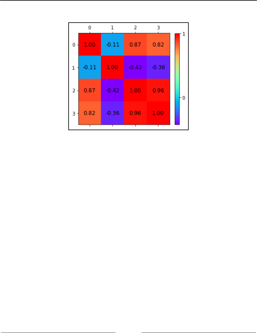
The Data Pipeline Chapter 3

[ 146 ]

Here is the resulting heat map:

From the previous diagram, you can see that the value of the primary diagonal is 1. This is

because we're using the normalized version of the covariance matrix (normalizing each

feature covariance to 1.0). We can also notice a high correlation between the first and the

third, the first and the fourth, and the third and the fourth features. In addition, we can

verify that only the second feature is almost independent of the others; all the other features

are somehow correlated to each other.

We now have an idea about the potential number of features in the reduced set, imagining

compressing the duplicated information as pointed out by the correlation matrix – we can

reduce everything simply to two features.

Principal component analysis

Principal component analysis (PCA) is a technique that helps define a smaller and more

relevant set of features. The new features obtained from PCA are linear combinations (that

is, rotation) of the current features, even if they are binary. After the rotation of the input

space, the first vector of the output set contains most of the signal's energy (or, in other

words, its variance). The second is orthogonal to the first, and it contains most of the

remaining energy; the third is orthogonal to the first two vectors and contains most of the

remaining energy, and so on. It's just like restructuring the information in the dataset by

aggregating as much as possible of the information onto the initial vectors produced by the

PCA.

The Data Pipeline Chapter 3

[ 147 ]

In the (ideal) case of AWGN, the initial vectors contain all of the information of the input

signal; the ones toward the end only contain noise. Moreover, since the output basis is

orthogonal, you can decompose and synthesize an approximate version of the input

dataset. The key parameter, which is used to decide how many basis vectors one can use, is

the energy. Since the algorithm, under the hood, is for singular value decomposition,

eigenvectors (the basis vectors) and eigenvalues (the standard deviation associated with

that vector) are two terms that are often referred to when reading about PCA. Typically, the

cardinality of the output set is the one that guarantees the presence of 95% (in some cases,

90 or 99% are needed) of the input energy (or variance). A rigorous explanation of PCA is

beyond the scope of this book, and hence, we will just inform you about the guidelines on

how to use this powerful tool in Python.

Here's an example on how to reduce the dataset to two dimensions. In the previous section,

we deduced that 2 was a good choice for a dimensionality reduction; let's check if we were

right:

In: from sklearn.decomposition import PCA

pca_2c = PCA(n_components=2)

X_pca_2c = pca_2c.fit_transform(iris.data)

X_pca_2c.shape

Out: (150, 2)

In: plt.scatter(X_pca_2c[:,0], X_pca_2c[:,1], c=iris.target, alpha=0.8,

s=60, marker='o', edgecolors='white')

plt.show()

pca_2c.explained_variance_ratio_.sum()

Out: 0.97763177502480336

The Data Pipeline Chapter 3

[ 148 ]

When executing the code, you also get a scatterplot of the first two components:

Scatterplot of the ﬁrst two components

We can immediately see that, after applying the PCA, the output set has only two features.

This is because the PCA() object was called with the n_components parameter set to 2. An

alternative way to obtain the same result would be to run PCA() for 1, 2, and 3 components

and then conclude from the explained variance ratio and the visual inspection that for

n_components = 2, we got the best result. Then, we will have evidence that when using

two basis vectors, the output dataset contains almost 98% of the energy of the input signal,

and in the schema, the classes are pretty much neatly separable. Each color is located in a

different area of the two dimensional Euclidean space.

Please note that this process is automatic and you don't need to provide

labels while training PCA. In fact, PCA is an unsupervised algorithm, and

it does not require data related to the independent variable to rotate the

projection basis.

For curious readers, the transformation matrix (which turns the initial dataset into the PCA-

restructured one) can be seen with the help of the following code:

In: pca2c.components

Out: array([[ 0.36158968, -0.08226889, 0.85657211, 0.35884393],

[-0.65653988, -0.72971237, 0.1757674 , 0.07470647]])

The Data Pipeline Chapter 3

[ 149 ]

The transformation matrix is comprised of four columns (which is the number of input

features) and two rows (which is the number of the reduced ones).

Sometimes, you will find yourself in a situation where PCA is not effective enough,

especially when dealing with high dimensionality data, since the features may be very

correlated and, at the same time, the variance is unbalanced. A possible solution for such a

situation is to try to whiten the signal (or make it more spherical). In this occurrence,

eigenvectors are forced to unit component-wise variances. Whitening removes information,

but sometimes it improves the accuracy of the machine learning algorithms that will be

used after the PCA's reduction. Here's what the code looks like when resorting to

whitening (in our example, it doesn't change anything except for the scale of the dataset

with the reduced output):

In: pca_2cw = PCA(n_components=2, whiten=True)

X_pca_1cw = pca_2cw.fit_transform(iris.data)

plt.scatter(X_pca_1cw[:,0], X_pca_1cw[:,1], c=iris.target, alpha=0.8,

s=60, marker='o', edgecolors='white')

plt.show()

pca_2cw.explained_variance_ratio_.sum()

Out: 0.97763177502480336

You also get the scatterplot of the first components of the PCA using whitening:

Now, let's see what happens if we project the input dataset on a 1-D space that's generated

with PCA, as follows:

In: pca_1c = PCA(n_components=1)

X_pca_1c = pca_1c.fit_transform(iris.data)

plt.scatter(X_pca_1c[:,0], np.zeros(X_pca_1c.shape),

c=iris.target, alpha=0.8, s=60, marker='o', edgecolors='white')

The Data Pipeline Chapter 3

[ 150 ]

plt.show()

pca_1c.explained_variance_ratio_.sum()

Out: 0.9246162071742684

The projection is distributed along a single horizontal line:

In this case, the output energy is lower (92.4% of the original signal), and the output points

are added to the mono-dimensional Euclidean space. This might not be a great feature

reduction step since many points with different labels are mixed together.

Finally, here's a trick. To ensure that you generate an output set

containing at least 95% of the input energy, you can just specify this value

to the PCA object during its first call. A result equal to the one with two

vectors can be obtained with the following code:

In: pca_95pc = PCA(n_components=0.95)

X_pca_95pc = pca_95pc.fit_transform(iris.data)

print (pca_95pc.explained_variance_ratio_.sum())

print (X_pca_95pc.shape)

Out: 0.977631775025

(150, 2)

The Data Pipeline Chapter 3

[ 151 ]

PCA for big data – RandomizedPCA

The main issue with PCA is the complexity of the underlying singular value

decomposition (SVD) algorithm that does the reduction work, making the whole process

very difficult to scale. There is a faster algorithm in Scikit-learn based on randomized SVD.

It is a lighter but approximate iterative decomposition method. Using randomized SVD, the

full-rank reconstruction is not perfect, and the basis vectors are optimized locally during

every iteration. On the other hand, it requires only a few steps to get a good approximation,

demonstrating how randomized SVD is much faster than the classical SVD algorithms.

Therefore, this reduction algorithm is a great choice if the training dataset is large. In the

following code, we will apply it to the Iris dataset. The output is pretty close to the classical

PCA since the size of the problem is very small. However, the results vary significantly

when the algorithm is applied to large datasets:

In: from sklearn.decomposition import PCA

rpca_2c = PCA(svd_solver='randomized', n_components=2)

X_rpca_2c = rpca_2c.fit_transform(iris.data)

plt.scatter(X_rpca_2c[:,0], X_rpca_2c[:,1],

c=iris.target, alpha=0.8, s=60, marker='o', edgecolors='white')

plt.show()

rpca_2c.explained_variance_ratio_.sum()

Out: 0.97763177502480414

Here is the scatterplot of the first two components of the PCA using SVD solver:

The Data Pipeline Chapter 3

[ 152 ]

Latent factor analysis

Latent factor analysis (LFA) is another technique that helps you reduce the dimensionality

of the dataset. The overall idea is similar to PCA. However, in this case, there's no

orthogonal decomposition of the input signal, and therefore, no output basis. Some data

scientists think that LFA is a generalization of PCA that removes the constraint of

orthogonality. Generally, LFA is used when a latent factor or a construct is expected to be

present in the system. Under such a hypothesis, all of the features are observations of

variables that are derived or influenced by the latent factor that is transformed linearly and

which has an arbitrary waveform generator (AWG) noise. It is generally assumed that the

latent factor has a Gaussian distribution and a unitary covariance. Therefore, in this case,

instead of collapsing the energy/variance of the signal, the covariance among the variables

is explained in the output dataset. The Scikit-learn toolkit implements an iterative

algorithm, making it suitable for large datasets.

Here's the code to lower the dimensionality of the Iris dataset by assuming two latent

factors in the system:

In: from sklearn.decomposition import FactorAnalysis

fact_2c = FactorAnalysis(n_components=2)

X_factor = fact_2c.fit_transform(iris.data)

plt.scatter(X_factor[:,0], X_factor[:,1],

c=iris.target, alpha=0.8, s=60,

marker='o', edgecolors='white')

plt.show()

Here are the two latent factors as represented in a scatterplot (a different solution than the

previous PCA):

The Data Pipeline Chapter 3

[ 153 ]

Linear discriminant analysis

Strictly speaking, linear discriminant analysis (LDA) is a classifier (a classical statistical

method developed by Ronald Fisher, the father of modern statistics), but it is often used for

dimensionality reduction. It doesn't scale so well to larger datasets (like many statistical

methods), but it's something to be tried, which could bring better results than other

classification methods such as logistic regression. Since it's a supervised approach, it

requires the label set to optimize the reduction step. LDA outputs linear combinations of

the input features, trying to model the difference between the classes that best discriminate

them (since LDA uses label information). Compared to PCA, the output dataset that is

obtained with the help of LDA contains a neat distinction between classes. However, it

cannot be used in regression problems, since it is derived from a classification process.

Here's the application of LDA on the Iris dataset:

In: from sklearn.lda import LDA

lda_2c = LDA(n_components=2)

X_lda_2c = lda_2c.fit_transform(iris.data, iris.target)

plt.scatter(X_lda_2c[:,0], X_lda_2c[:,1],

c=iris.target, alpha=0.8, edgecolors='none')

plt.show()

This scatterplot is derived from the first two components generated by the LDA:

The Data Pipeline Chapter 3

[ 154 ]

Latent semantical analysis

Typically, latent semantical analysis (LSA) is applied to text after it has been processed by

TfidfVectorizer or CountVectorizer. Compared to PCA, it applies SVD to the input

dataset (which is usually a sparse matrix), producing semantic sets of words that are

usually associated with the same concept. This is why LSA is used when the features are

homogeneous (that is, all the words in the documents) and are present in large numbers.

An example of the same in Python with text and TfidfVectorizer is as follows. The

output shows part of the content of a latent vector:

In: from sklearn.datasets import fetch_20newsgroups

categories = ['sci.med', 'sci.space']

twenty_sci_news = fetch_20newsgroups(categories=categories)

from sklearn.feature_extraction.text import TfidfVectorizer

tf_vect = TfidfVectorizer()

word_freq = tf_vect.fit_transform(twenty_sci_news.data)

from sklearn.decomposition import TruncatedSVD

tsvd_2c = TruncatedSVD(n_components=50)

tsvd_2c.fit(word_freq)

arr_vec = np.array(tf_vect.get_feature_names())

arr_vec[tsvd_2c.components_[20].argsort()[-10:][::-1]]

Out: array(['jupiter', 'sq', 'comet', 'of', 'gehrels', 'zisfein',

'jim', 'gene', 'are', 'omen'], dtype='<U79')

Independent component analysis

As you can guess from the name, independent component analysis (ICA) is an approach

where you try to derive independent components from the input signal. In fact, ICA is a

technique that allows you to create maximally independent additive subcomponents from

the initial multivariate input signal. The main hypothesis of this technique focuses on the

statistical independence of the subcomponents and their non-Gaussian distribution. ICA

has a lot of applications in neurological data and is widely used in the neuroscience

domain.

The Data Pipeline Chapter 3

[ 155 ]

A typical scenario that may require the use of ICA is blind source separation. For example,

two or more microphones will record two sounds (for instance, a person speaks and a song

plays at the same time). In this case, ICA is able to separate the two sounds into two output

features.

The Scikit-learn package offers a faster version of the algorithm

(sklearn.decomposition.FastICA), whose use is similar to the other techniques that

have been presented thus far.

Kernel PCA

Kernel PCA is a technique that uses a kernel to map the signal on a (typically) nonlinear

space and makes it linearly separable (or close to attaining the same). It's an extension of

PCA, where the mapping is an actual projection on a linear subspace. There are many well-

known kernels (and of course, you can always build your own on the fly), but the most

used ones are linear, poly, RBF, sigmoid, and cosine. They all serve different configurations of

input datasets as they are only able to linearize some selected types of data. For example,

let's imagine that we have a disk-shaped dataset, like the one we are going to create with

the following code:

In: def circular_points (radius, N):

return np.array([[np.cos(2*np.pi*t/N)*radius,

np.sin(2*np.pi*t/N)*radius] for t in range(N)])

N_points = 50

fake_circular_data = np.vstack([circular_points(1.0, N_points),

circular_points(5.0, N_points)])

fake_circular_data += np.random.rand(*fake_circular_data.shape)

fake_circular_target = np.array([0]*N_points + [1]*N_points)

plt.scatter(fake_circular_data[:,0], fake_circular_data[:,1],

c=fake_circular_target, alpha=0.8,

s=60, marker='o', edgecolors='white')

plt.show()

The Data Pipeline Chapter 3

[ 156 ]

Here is the output of the example:

With this input dataset, all the linear transformations will fail to separate blue and red dots,

since the dataset contains circumference-shaped classes. Now, let's try this with the Kernel

PCA by using an RBF kernel and see what happens:

In: from sklearn.decomposition import KernelPCA

kpca_2c = KernelPCA(n_components=2, kernel='rbf')

X_kpca_2c = kpca_2c.fit_transform(fake_circular_data)

plt.scatter(X_kpca_2c[:,0], X_kpca_2c[:,1], c=fake_circular_target,

alpha=0.8, s=60, marker='o', edgecolors='white')

plt.show()

The following figure represents the transformation of the example:

The Data Pipeline Chapter 3

[ 157 ]

Graphs/diagrams in this chapter may be different to the ones obtained on

your local computer because graphical layout initialization is made with

random parameters.

We achieved our goal – the blue dots are on the left and the red dots are on the right.

Thanks to the Kernel PCA's transformation, you can now deal with this dataset by using

linear techniques.

T-SNE

PCA is a widespread technique for dimensionality reduction, yet when we deal with large

data, presenting many features, we first need to understand what's going on in the feature

space. In fact, in the EDA phase, you'll usually make several scatterplots of the data to

understand what the relationship between features is. At this point, T-distributed stochastic

neighbor embedding, or T-SNE, comes to your aid since it has been designed with the goal

of embedding high-dimensional data in a 2-D or 3-D space to make the most of a

scatterplot. It is a nonlinear dimensionality reduction technique developed by Laurens van

der Maaten and Geoffrey Hinton and the core of the algorithm is based on two rules: the

first is that recurrent similar observations must have a greater contribution to the output

(and that's achieved with a probability distribution function); second, the distribution in the

high-dimensional space must be similar to the one in the small space (and that's achieved

by minimizing the Kullback-Leibler (KL), divergence between the two probability

distribution functions). The output is visually nice and allows you to guess nonlinear

interactions between features.

Let's see how a simple example works by applying the T-SNE to the Iris dataset and

plotting it to a two-dimensional space:

In: from sklearn.manifold import TSNE

from sklearn.datasets import load_iris

iris = load_iris()

X, y = iris.data, iris.target

X_tsne = TSNE(n_components=2).fit_transform(X)

plt.scatter(X_tsne[:, 0], X_tsne[:, 1], c=y, alpha=0.8,

s=60, marker='o', edgecolors='white')

plt.show()

The Data Pipeline Chapter 3

[ 158 ]

Here is the result from the T_SNE, completely separating one class from the others:

Restricted Boltzmann Machine

The Restricted Boltzmann Machine (RBM) is another technique that, composed of linear

functions (which are usually called hidden units or neurons), creates a nonlinear

transformation of the input data. The hidden units represent the status of the system, and

the output dataset is actually the status of that layer.

The main hypothesis of this technique is that the input dataset is composed of features that

represent probability (binary values or real values in the [0,1] range), since RBM is a

probabilistic approach. In the following example, we will feed the RBM using binarized

pixels of images as features (1=white, 0=black), and we will print the latent components of

the system. These components represent different generic faces that appear in the original

images:

In: from sklearn import preprocessing

from sklearn.neural_network

import BernoulliRBM

n_components = 64 # Try with 64, 100, 144

olivetti_faces = datasets.fetch_olivetti_faces()

X = preprocessing.binarize(

preprocessing.scale(olivetti_faces.data.astype(float)),

0.5)

rbm = BernoulliRBM(n_components=n_components, learning_rate=0.01,

n_iter=100)

rbm.fit(X)

plt.figure(figsize=(4.2, 4))

for i, comp in enumerate(rbm.components_):

The Data Pipeline Chapter 3

[ 159 ]

plt.subplot(int(np.sqrt(n_components+1)),

int(np.sqrt(n_components+1)), i + 1)

plt.imshow(comp.reshape((64, 64)), cmap=plt.cm.gray_r,

interpolation='nearest')

plt.xticks(()); plt.yticks(())

plt.suptitle(str(n_components) + ' components extracted by RBM',

fontsize=16)

plt.subplots_adjust(0.08, 0.02, 0.92, 0.85, 0.08, 0.23)

plt.show()

Here are the 64 components extracted by RBM:

Note that Scikit-learn contains just the base layer of RBM processing. If

you are working on big datasets, you are better off using GPU-based

toolkits (such as the ones built on the top of CUDA or OpenCL) since

RBMs are highly parallelizable.

The detection and treatment of outliers

In data science, examples are at the core of learning from data processes. If unusual,

inconsistent, or erroneous data is fed into the learning process, the resulting model may be

unable to generalize the accommodation of any new data correctly. An unusually high

value present in a variable, apart from skewing descriptive measures such as the mean and

variance, may also distort how many machine learning algorithms learn from data, causing

distorted predictions as a result.

The Data Pipeline Chapter 3

[ 160 ]

When a data point deviates markedly from the others in a sample, it is called an outlier. Any

other expected observation is labeled as an inlier.

A data point may be an outlier due to the following three general causes (and each one

implies different remedies):

The point represents a rare occurrence, but it is also a possible value, given the

fact that the available data is just a sample of the original data distribution. In

such an occurrence, the generative underlying process is the same for all the

points, but the outlying point may be deemed as unsuitable for a generalization

by machine learning due to its rarity. In such a case, the point is commonly

removed or underweighted. Another solution is to increase the sample number,

thus making the unusual value less relevant in the dataset.

The point represents the usual occurrence of another distribution. When similar

situations occur, it is plausible to imagine an error or a misspecification that has

affected the generation of the sample. In any case, your learning algorithm is

going to learn from data coming from an extraneous distribution that is not the

focus of interest of your data science project (the focus is on the generalization).

In such a case, the outlier simply has to be removed.

The point is clearly some kind of a mistake. For some reason, there has been a

data entry error or a problem with data integrity that modified the original value

and replaced it with an inconsistent value. The best course of action is to remove

the value and treat it as a value that is missing at random. In this case, it is

common to replace the outlier with a mean or the most common class depending

on whether it is a regression or a classification problem. If it is not convenient or

possible to do so, then we suggest that you just remove the example from the

dataset.

Univariate outlier detection

To explain the reason behind why a data point is an outlier, you are first required to locate

the possible outliers in your data. There are quite a few approaches – some are univariate

(you can observe each singular variable at once), while the others are multivariate (they

consider more variables at the same time). The univariate methods are usually based on

EDA and visualizations such as boxplots (which have been introduced at the beginning of

the present chapter; we will talk more about boxplots more specifically in Chapter 5,

Visualization, Insights, and Results).

The Data Pipeline Chapter 3

[ 161 ]

There are a couple of rules of thumb to keep in mind when chasing outliers by examining

single variables. In fact, outliers may be spotted as extreme values:

If you are observing Z-scores, observations with scores higher than 3 in an

absolute value have to be considered as suspect outliers.

If you are observing a description of data, you can consider the observations that

are smaller than the 25th percentile value minus the IQR (that is, the difference

between the 75th and 25th percentile values) as suspect outliers – *1.5 and those

greater than the 75th percentile value plus the IQR * 1.5. Usually, you can achieve

such distinction with the help of a boxplot graph.

In order to present how we can easily detect some outliers using Z-scores, let's load and

explore the Boston House Prices dataset. As pointed out by the description of the dataset

(which you can get with the help of boston.DESCR), the variable CHAS, which is indexed

as 3, is a binary. Therefore, it makes little sense to use it while detecting anomalous values.

In fact, such a variable can have just a value of either 0 or 1:

In: from sklearn.datasets import load_boston

boston = load_boston()

continuous_variables = [n for n in range(boston.data.shape[1]) if n!=3]

Now, let's quickly standardize all the continuous variables by using the StandardScaler

function from sklearn. Our target is the fancy indexing of boston.data

boston.data[:,continuous_variables] in order to create another array containing all

the variables except the previous one, which was indexed 3.

StandardScaler automatically standardizes to zero mean and unit variance. This is a

necessary routine operation that should be performed before feeding the data to the

learning phase. Otherwise, many algorithms won't work properly (such as linear models

Finally, let's locate the values that are above the absolute value of three standard

deviations:

In: import numpy as np

from sklearn import preprocessing

scaler= preprocessing.StandardScaler()

normalized_data = scaler.fit_transform(

boston.data[:,continuous_variables])

outliers_rows, outliers_columns = np.where(np.abs(normalized_data)>3)

The Data Pipeline Chapter 3

[ 162 ]

The outliers_rows and outliers_columns variables contain the row and column

indexes of the suspect outliers. We can print the index of the examples:

In: print(outliers_rows)

Out: [ 55 56 57 102 141 199 200 201 202 203 204 225 256 257 262 283 284

...

Alternatively, we can display the tuple of the row/column coordinates in the array:

In: print (list(zip(outliers_rows, outliers_columns)))

Out: [(55, 1), (56, 1), (57, 1), (102, 10), (141, 11), (199, 1), (200, 1),

...

The univariate approach can reveal quite a lot of potential outliers. It won't disclose an

outlier that does not have an extreme value – instead, it is characterized by an unusual

combination of values in two or more variables. In such cases, the values of the involved

variables may not even be extreme ones, and therefore, the outlier may slip away unnoticed

by a univariate inspection. These outliers are called multivariate outliers.

In order to discover multivariate outliers, you can use a dimensionality reduction

algorithm, such as the previously illustrated PCA, and then check the absolute values of the

components that are beyond three standard deviations, or visually inspect bivariate plots in

order to locate isolated clusters of data points.

The Scikit-learn package offers a couple of classes that can automatically work for you

straight out of the box and signal all suspect cases:

The covariance.EllipticEnvelope class fits a robust distribution estimation

of your data, pointing out the outliers that might be contaminating your dataset

because they are the extreme points in the general distribution of the data.

The svm.OneClassSVM class is a support vector machine algorithm that can

approximate the shape of your data and find out if any new instances provided

should be considered as a novelty (it acts as a novelty detector because, by

default, it presumes that there is no outlier in the data). By just modifying its

parameters, it can also work on a dataset where outliers are present, providing

an even more robust and reliable outlier detection system than

EllipticEnvelope.

Both classes, based on different statistical and machine learning approaches, need to be

known and applied during your modeling phase.

The Data Pipeline Chapter 3

[ 163 ]

EllipticEnvelope

EllipticEnvelope is a function that tries to figure out the key parameters of your data's

general distribution by assuming that your entire data is an expression of an underlying

multivariate Gaussian distribution. That's an assumption that cannot hold true for all

datasets, yet when it does, it proves an effective method indeed for spotting outliers.

Simplifying the complex estimations working behind the algorithm as much as possible, we

can say that it checks the distance of each observation with respect to a grand mean that

takes into account all the variables in your dataset. For this reason, it is able to spot both

univariate and multivariate outliers.

The only parameter that you have to take into account when using this function from the

covariance module is the contamination parameter, which can take a value of up to 0.5. It

provides information to the algorithm about the proportion of the outliers present in your

dataset. Situations may vary from dataset to dataset. However, as a starting figure, we

suggest a value from 0.01 - 0.02 since it is the percentage of observations that should fall

over the absolute value 3 in the Z score distance from the mean in a standardized normal

distribution. For this reason, we deem the default value of 0.1 as too high.

Let's see this algorithm in action with the help of a synthetic distribution:

In: from sklearn.datasets import make_blobs

blobs = 1

blob = make_blobs(n_samples=100, n_features=2, centers=blobs,

cluster_std=1.5, shuffle=True, random_state=5)

# Robust Covariance Estimate

from sklearn.covariance import EllipticEnvelope

robust_covariance_est = EllipticEnvelope(contamination=.1).fit(blob[0])

detection = robust_covariance_est.predict(blob[0])

outliers = np.where(detection==-1)[0]

inliers = np.where(detection==1)[0]

# Draw the distribution and the detected outliers

from matplotlib import pyplot as plt

# Just the distribution

plt.scatter(blob[0][:,0],blob[0][:,1], c='blue', alpha=0.8, s=60,

marker='o', edgecolors='white')

plt.show()

# The distribution and the outliers

in_points = plt.scatter(blob[0][inliers,0],blob[0][inliers,1],

c='blue', alpha=0.8,

s=60, marker='o',

edgecolors='white')

out_points = plt.scatter(blob[0][outliers,0],blob[0][outliers,1],

c='red', alpha=0.8,

s=60, marker='o',

edgecolors='white')

The Data Pipeline Chapter 3

[ 164 ]

plt.legend((in_points,out_points),('inliers','outliers'),

scatterpoints=1,

loc='lower right')

plt.show()

Let's examine this code closely.

The make_blobs function creates a certain number of distributions in a bidimensional

space for a total of 100 examples (the n_samples parameter). The number of distributions

(parameter centers) is related to the user-defined variable blobs, which is initially set to 1.

After creating the artificial example data, running EllipticEnvelope with a

contamination rate of 10% helps you find out the extreme values in the distribution. The

model first deploys the fit by using the .fit() method on the EllipticEnvelope class.

Then, a prediction is obtained by using the .predict() method on the data that was used

for the fit.

The results, corresponding to a vector of values 1 and -1 (with -1 being the mark for

anomalous examples), can be displayed thanks to a couple of scatterplots by using the plot

function from the pyplot module in matplotlib.

The distinction between inliers and outliers is recorded in the variable's outliers and inliers,

which contain the indexes of the examples.

Now, let's run the code a few more times after changing the number of blobs and examine

the results when the blobs have a value of 1 and 4:

The Data Pipeline Chapter 3

[ 165 ]

The distributions of data points after changing the number of blobs is as follows:

In the case of a unique, underlying multivariate distribution (when the variable blobs = 1),

the EllipticEnvelope algorithm has successfully located 10% of the observations on the

fringe of the distribution itself and has consequently signaled all the suspect outliers.

Instead, when multiple distributions are present in the data as if there were two or more

natural clusters, the algorithm, trying to fit a unique general distribution, tends to locate the

potential outliers on just the most remote cluster, thus ignoring other areas of data that

might be potentially affected by outlying cases.

This is not an unusual situation with real data, and it represents an important limitation of

the EllipticEnvelope algorithm.

Now, let's get back to our initial Boston House Prices dataset for the verification of some

more data that is more realistic than our synthetic blobs. Here is the first part of the code

that we can use for our experiment:

In: from sklearn.decomposition import PCA

# Normalized data relative to continuos variables

continuous_variables = [n for n in range(boston.data.shape[1]) if n!=3]

scaler = preprocessing.StandardScaler()

normalized_data = scaler.fit_transform(

boston.data[:,continuous_variables])

# Just for visualization purposes pick the first 2 PCA components

pca = PCA(n_components=2)

Zscore_components = pca.fit_transform(normalized_data)

vtot = 'PCA Variance explained ' + str(round(np.sum(

The Data Pipeline Chapter 3

[ 166 ]

pca.explained_variance_ratio_),3))

v1 = str(round(pca.explained_variance_ratio_[0],3))

v2 = str(round(pca.explained_variance_ratio_[1],3))

In this script, we will first standardize the data and then, just for subsequent visualization

purposes, generate a reduction of two components by using PCA.

The two PCA components account for about 62% of the initial variance that is expressed by

the 12 continuous variables that are available in the dataset (the summed value of the

.explained_variance_ratio_ variable, which is internal to the fitted PCA class).

Although only two PCA components are sufficient for visualization purposes, normally,

you'd get more than two components for this dataset since the target is to have enough to

account for at least 95% of the total variance (as stated previously in this chapter).

We will continue with the script:

In: robust_covariance_est = EllipticEnvelope(store_precision=False,

assume_centered = False,

contamination=.05)

robust_covariance_est.fit(normalized_data)

detection = robust_covariance_est.predict(normalized_data)

outliers = np.where(detection==-1)

regular = np.where(detection==1)

In: # Draw the distribution and the detected outliers

from matplotlib import pyplot as plt

in_points = plt.scatter(Zscore_components[regular,0],

Zscore_components[regular,1],

c='blue', alpha=0.8, s=60, marker='o',

edgecolors='white')

out_points = plt.scatter(Zscore_components[outliers,0],

Zscore_components[outliers,1],

c='red', alpha=0.8, s=60, marker='o',

edgecolors='white')

plt.legend((in_points,out_points),('inliers','outliers'),

scatterpoints=1, loc='best')

plt.xlabel('1st component ('+v1+')')

plt.ylabel('2nd component ('+v2+')')

plt.xlim([-7,7])

plt.ylim([-6,6])

plt.title(vtot)

plt.show()

The Data Pipeline Chapter 3

[ 167 ]

The visualization of the first two components accounts for 62.2% of the original variance:

As in the previous example, where we assumed a low contamination that is equivalent to

0.05, the code based on EllipticEnvelope predicts the outliers and stores them in an

array in the same way as it stores the inliers. Finally, there's the visualization (as mentioned

previously, we are going to discuss all of the visualization methods in Chapter 5,

Visualization, Insights, and Results).

Now, let's observe the result offered by the scatterplot we generated to visualize the first

two PCA components of the data and mark the outlying observations. Concerning the

general distribution of the data points in our example, as provided by the two components

that account for about 62% of the variance in the data, it appears as if there are two distinct

clusters of house prices in Boston, which correspond to the high-end and low-end units

present in the market. Generally speaking, the presence of clusters in the data is a no

optimal situation for EllipticEnvelope estimations. In fact, according to what we've

already noticed while experimenting using synthetic blobs, the algorithm has pointed out

the outliers on just a cluster – the lesser one. Given such results, there is a strong reason to

believe that we just received a biased, partial response, and some further investigation will

be required before deeming such points as outliers. The Scikit-learn package actually

integrates the robust covariance estimation method, which is fundamentally a statistical

approach, with another methodology that is well-rooted in machine learning: the

OneClassSVM class. Now, we will move on to experimenting with it.

The Data Pipeline Chapter 3

[ 168 ]

Before leaving this example, please note that to fit both PCA and

EllipticEnvelope, we used an array named normalized_data, which

contains just the standardized continuous dataset variables. Please always

take into account that using nonstandardized data and mixing binary or

categorical data with continuous ones may induce errors and

approximated estimations for the EllipticEnvelope algorithm.

OneClassSVM

As EllipticEnvelope fits a hypothetical Gaussian distribution, leveraging parametric

and statistical assumptions, OneClassSVM is a machine learning algorithm that learns what

the distribution of the features should be from the data itself, and therefore is applicable in

a large variety of situations when you want to be able to catch all the outliers but also the

unusual data examples.

It is great if you already have a clean dataset and have it fitted by machine learning

algorithms. Afterwards, OneClassSVM can be summoned to check if any new example fits

in the historical distribution, and if it doesn't, it will signal a novel example, which might be

both an error or some new, previously unseen situation.

Just think of data science situations as a machine learning classification algorithm trained to

recognize posts and news on a website and take online actions. OneClassSVM can easily

spot a post that is different from the others present on the website (spam, maybe?), whereas

other algorithms will just try to fit the new example into the existing topic's categorization.

However, OneClassSVM can also be used to spot existing outliers. If this specialized SVM

class cannot fit some data, which is pointed out as being at the margins of the data

distribution, then there is surely something fishy about those examples.

In order to have OneClassSVM work as an outlier detector, you need to work on its core

parameters; it requires you to define the kernel, degree, gamma, and nu:

Kernel and degree: These are interconnected. Usually, the values that we suggest

based on our experience are the default ones; the type of kernel should be rbf

and its degree should be 3. Such parameters will inform OneClassSVM to create a

series of classification bubbles that span through three dimensions, allowing you

to model even the most complex multidimensional distribution forms.

The Data Pipeline Chapter 3

[ 169 ]

Gamma: This is a parameter that's connected to the RBF kernel. We suggest that

you keep it as low as possible. A good rule of thumb should be to assign it a

minimum value that lies between the inverse of the number of cases and the

variables. The role of gamma in SVM will be explained further in Chapter 4,

Machine Learning. It will suffice for now to say that higher values of gamma tend

to lead the algorithm to follow the data, but more so define the shape of the

classification bubbles.

Nu: This parameter determines whether we have to fit the exact distribution or if

we try to obtain a certain degree of generalization by not adapting too much to

the present data examples (a necessary choice if outliers are present). It can be

easily determined with the help of the following formula:

nu_estimate = 0.95 * outliers_fraction + 0.05

If the value of the outliers' fraction is very small, nu will be small and the SVM

algorithm will try to fit the contour of the data points. On the other hand, if the

fraction is high, so will the parameter be, forcing a smoother boundary of the

inliers' distributions.

Let's immediately observe the performance of this algorithm on the problem that we faced

before on the Boston House Prices dataset:

In: from sklearn.decomposition import PCA

from sklearn import preprocessing

from sklearn import svm

# Normalized data relative to continuos variables

continuous_variables = [n for n in range(boston.data.shape[1]) if n!=3]

scaler = preprocessing.StandardScaler()

normalized_data = scaler.fit_transform(

boston.data[:,continuous_variables])

# Just for visualization purposes pick the first 5 PCA components

pca = PCA(n_components=5)

Zscore_components = pca.fit_transform(normalized_data)

vtot = 'PCA Variance explained ' + str(round(

np.sum(pca.explained_variance_ratio_),3))

# OneClassSVM fitting and estimates

outliers_fraction = 0.02 #

nu_estimate = 0.95 * outliers_fraction + 0.05

machine_learning = svm.OneClassSVM(kernel="rbf",

gamma=1.0/len(normalized_data),

degree=3, nu=nu_estimate)

machine_learning.fit(normalized_data)

detection = machine_learning.predict(normalized_data)

outliers = np.where(detection==-1)

The Data Pipeline Chapter 3

[ 170 ]

regular = np.where(detection==1)

We will now proceed to visualize the results:

In: # Draw the distribution and the detected outliers

from matplotlib import pyplot as plt

for r in range(1,5):

in_points = plt.scatter(Zscore_components[regular,0],

Zscore_components[regular,r],

c='blue', alpha=0.8, s=60,

marker='o', edgecolors='white')

out_points = plt.scatter(Zscore_components[outliers,0],

Zscore_components[outliers,r],

c='red', alpha=0.8, s=60,

marker='o', edgecolors='white')

plt.legend((in_points,out_points),('inliers','outliers'),

scatterpoints=1, loc='best')

plt.xlabel('Component 1 (' + str(round(

pca.explained_variance_ratio_[0],3))+')')

plt.ylabel('Component '+str(r+1)+'('+str(round(

pca.explained_variance_ratio_[r],3))+')')

plt.xlim([-7,7])

plt.ylim([-6,6])

plt.title(vtot)

plt.show()

Compared to the code presented previously, this snippet is different because the resulting

PCA decomposition is made up of five components. The larger number is due in order to

explore more data dimensions. Another reason for increasing the number of resulting PCA

components is because of our intention to use the transformed dataset with OneClassSVM.

The core parameters are calculated from the number of observations, as follows:

gamma=1.0/len(normalized_data)

nu=nu_estimate

In particular, nu depends on:

nu_estimate = 0.95 * outliers_fraction + 0.05

So, by changing the outliers_fraction (from 0.02 to a larger value, such as 0.1), you

require the algorithm to give more attention to possible anomalies when supposing a larger

incidence of anomalous cases in your data.

The Data Pipeline Chapter 3

[ 171 ]

Let's also observe the graphical output of PCA components from 2 to 5 and compare it with

the principal component (51% of the explained variance). The first graph of the series

(comprised of a total of four scatterplots) is as follows:

From our graphical exploration, it looks as if OneClassSVM modeled the distribution of

house price data with a good fit and it helped spot a few extreme values on the borders of

the distribution.

At this point, you can decide on one of the novelties and outlier detection approaches that

we are about to propose. You may even use both:

To scrutinize the characteristics of the outliers in order to figure out a reason for

their presence (a fact that could further make you reflect on the generative

processes underlying your data)

To try to build some machine learning models by using under-weighting for the

outlying observations or by just excluding them

In the end, with a pure data science approach, what will help you decide what to do next

with any outlying observation is testing the results of your decisions and consequent

operations on data. How to test and experiment with a hypothesis about your data is a

topic that we are going to discuss with you in the upcoming sections.

The Data Pipeline Chapter 3

[ 172 ]

Validation metrics

In order to evaluate the performance of the data science system that you have built and

check how close you are to the goal that you have in mind, you need to use a function that

scores the outcome. Typically, different scoring functions are used to deal with binary

classification, multilabel classification, regression, or a clustering problem. Now, let's see

the most popular functions for each of these tasks and how they are used by machine

learning algorithms.

Learning how to choose the right score/error measure for your data

science project is really a matter of experience. We found it very helpful to

consult (and participate in) the data science competitions held by Kaggle

(kaggle.com), a company devoted to organizing data challenges between

data scientists from all over the world. By observing the various

challenges and what score or error measure they try to optimize, you can

surely get useful insights for your own problems. Kaggle's CTO, Ben

Hammer, has even created a Python library of commonly used metrics in

competitions, which you can consult at github.com/benhamner/Metrics

and install on your computer by using pip install ml_metrics.

Multilabel classification

When your task is to predict more than a single label (for instance: What's the weather like

today? Which flower is this? What's your job?), we call the problem a multilabel

classification. Multilabel classification is a very popular task, and many performance

metrics exist to evaluate classifiers. Of course, you can use all of these measures in the case

of a binary classification. Now, let's explain how it works by using a simple, real-world

example:

In: from sklearn import datasets

iris = datasets.load_iris()

# No crossvalidation for this dummy notebook

from sklearn.model_selection import train_test_split

X_train, X_test, Y_train, Y_test = train_test_split(iris.data,

iris.target, test_size=0.50, random_state=4)

# Use a very bad multiclass classifier

from sklearn.tree import DecisionTreeClassifier

classifier = DecisionTreeClassifier(max_depth=2)

classifier.fit(X_train, Y_train)

Y_pred = classifier.predict(X_test)

iris.target_names

Out: array(['setosa', 'versicolor', 'virginica'], dtype='<U10')

The Data Pipeline Chapter 3

[ 173 ]

Now, let's take a look at the measures that are commonly used in multilabel classification:

Confusion matrix: Before we describe the performance metrics for multilabel

classification, let's take a look at the confusion matrix, a table that gives us an

idea about what the misclassifications are for each class. Ideally, in a perfect

classification, all the cells that are not on the diagonal should be 0s. In the

following example, you will instead see that class 0 (Setosa) is never misclassified,

class 1 (Versicolor) is misclassified twice as Virginica, and class 2 (Virginica) is

misclassified twice as Versicolor:

In: from sklearn import metrics

from sklearn.metrics import confusion_matrix

cm = confusion_matrix(y_test, y_pred)

print cm

Out: [[30 0 0]

[ 0 19 3]

[ 0 2 21]]

In: import matplotlib.pyplot as plt

img = plt.matshow(cm, cmap=plt.cm.autumn)

plt.colorbar(img, fraction=0.045)

for x in range(cm.shape[0]):

for y in range(cm.shape[1]):

plt.text(x, y, "%0.2f" % cm[x,y],

size=12, color='black', ha="center", va="center")

plt.show()

The confusion matrix is represented graphically in this way:

The Data Pipeline Chapter 3

[ 174 ]

Accuracy: Accuracy is the portion of the predicted labels that are exactly equal to

the real ones. In other words, it's the percentage of overall correctly classified

labels:

In: print ("Accuracy:", metrics.accuracy_score(Y_test, Y_pred))

Out: Accuracy: 0.933333333333

Precision: It is a measure that is taken from the information retrieval world. It

counts the number of relevant results in the result set. Equivalently, in a

classification task, it counts the number of correct labels in each set of classified

labels. Then, results are averaged on all of the labels:

In: print ("Precision:", metrics.precision_score(y_test, y_pred))

Out: Precision: 0.933333333333

Recall: This is another concept taken from information retrieval. It counts the

number of relevant results in the result set, compared to all of the relevant labels

in the dataset. In classification tasks, this is the amount of correctly classified

labels in the set divided by the total count of labels for that set. Finally, the results

are averaged, just like in the following code:

In: print ("Recall:", metrics.recall_score(y_test, y_pred))

Out: Recall: 0.933333333333

F1 Score: This is the harmonic average of precision and recall, which is mostly

used when dealing with unbalanced datasets in order to reveal if the classifier is

performing well with all the classes:

In: print ("F1 score:", metrics.f1_score(y_test, y_pred))

Out: F1 score: 0.933267359393

These are the most used measures in multilabel classification. A convenient function,

classification_report, shows a report on these measures, which is very handy.

Support is simply the number of observations with that label. It's pretty useful to

understand whether a dataset is balanced (that is, whether it has the same share of

examples for every class) or not:

In: from sklearn.metrics import classification_report

print classification_report(y_test, y_pred,

target_names=iris.target_names)

The Data Pipeline Chapter 3

[ 175 ]

Here is the complete report with precision, recall, f1-score and support (the number of

cases for the class):

In data science practice, precision and recall are used more extensively than accuracy, as

most datasets in data problems tend to be unbalanced. To account for this imbalance, data

scientists often present their results in terms of precision, recall, and f1-score. In addition,

we have to notice how accuracy, precision, recall, and f1-score assume values in the [0.0,

1.0] range. Perfect classifiers achieve the score of 1.0 for all of these measures (but beware of

any perfect classification if it's too good to believe, as this usually means that something

wrong has happened; real-world data problems never have a perfect solution).

Binary classification

In addition to the error measures shown in the preceding section, in problems where you

have only two output classes (for instance, if you have to guess the gender of a user or

predict whether the user will click/buy/like the item), there are some additional measures.

The most used one, since it's very informative, is the area under the receiver operating

characteristics curve (ROC) or area under a curve (AUC).

The ROC curve is a graphical way to express how the performances of the classifier change

over all the possible classification thresholds (that is, changes in the outcome when its

parameters change). Specifically, these performances have a true positive (or hit) rate and a

false positive (or miss) rate. The first is the rate of the correct positive results, and the

second is the rate of the incorrect ones. The area under that curve represents how well the

classifier performs with respect to a random classifier (whose AUC is 0.50).

The Data Pipeline Chapter 3

[ 176 ]

Here, we have a graphical example of a random classifier (dotted line) and a better one

(solid line). You can see that the AUC of a random classifier is 0.5 (it is half of the square),

and the other has a higher AUC (with its upper bound at 1.0):

The function that is used to compute the AUC with Python is

sklearn.metrics.roc_auc_score().

Regression

In tasks where you have to predict real numbers or regression, many error measures are

derived from Euclidean algebra:

Mean absolute error or MAE: This is the mean L1 norm of the difference vector

between the predicted and real values:

In: from sklearn.metrics import mean_absolute_error

mean_absolute_error([1.0, 0.0, 0.0], [0.0, 0.0, -1.0])

Out: 0.66666666666666663

The Data Pipeline Chapter 3

[ 177 ]

Mean squared error or MSE: This is the mean L2 norm of the difference vector

between the predicted and real values:

In: from sklearn.metrics import mean_squared_error

mean_squared_error([-10.0, 0.0, 0.0], [0.0, 0.0, 0.0])

Out: 33.333333333333

score: R

is also known as the coefficient of determination. In a nutshell, R

determines how good a linear fit there is that exists between the predictors and

the target variable. It takes values between 0 and 1 (inclusive); the higher R

is,

the better the model. It is a good score measure, yet it doesn't tell everything

about the story, especially if there are outliers in your data. There are even more

intricacies about this metric that you can find in reference books on Statistics. As

a suggestion, use it, but accompany it with other score or error measurements.

The function to use in this case is sklearn.metrics.r2_score.

Testing and validating

After loading our data, preprocessing it, creating new, useful features, checking for outliers

and other inconsistent data points, and finally choosing the right metric, we are ready to

apply a machine learning algorithm.

A machine learning algorithm, by observing a series of examples and pairing them with

their outcome, is able to extract a series of rules that can be successfully generalized to new

examples by correctly guessing their resulting outcome. Such is the supervised learning

approach, where it applies a series of highly specialized learning algorithms that we expect

can correctly predict (and generalize) on any new data.

But how can we correctly apply the learning process in order to achieve the best model for

prediction to be generally used with similar yet new data?

In data science, there are some best practices to be followed that can assure you the best

results in the future generalization of your model to any new data. Let's explain this

practice by proceeding step by step, first loading the dataset that we will be working on in

the following example:

In: from sklearn.datasets import load_digits

digits = load_digits()

print (digits.DESCR)

X = digits.data

y = digits.target

The Data Pipeline Chapter 3

[ 178 ]

The digit dataset contains images of handwritten numbers from 0 to 9. The data format

consists of a matrix of 8 x 8 images of this kind:

These digits are actually stored as a vector (resulting from the flattening of each 8 x 8

image) of 64 numeric values from 0 to 16, representing grayscale tonality for each pixel:

In: X[0]

Out: array([0., 0., 5., 13., 9., 1., 0., 0., ...])

We will also upload three different machine learning hypotheses (a hypothesis, in machine

learning language, is an algorithm that's complete with all of its parameters set ready for

learning) using three different support vector machines for classification. They will be

useful for our practical example:

In: from sklearn import svm

h1 = svm.LinearSVC(C=1.0)

h2 = svm.SVC(kernel='rbf', degree=3, gamma=0.001, C=1.0)

h3 = svm.SVC(kernel='poly', degree=3, C=1.0)

As a first experiment, let's fit the linear SVM classifier to our data and verify the results:

In: h1.fit(X,y)

print (h1.score(X,y))

Out: 0.984974958264

The first method fits a model by using the X array in order to correctly predict one of the 10

classes indicated by the y vector. After that, by calling the .score() method and

specifying the same predictors (the X array), the method evaluates the performance in terms

of mean accuracy with respect to the true values given by the y vector. The result is about

98.5% accurate in predicting the correct digit.

The Data Pipeline Chapter 3

[ 179 ]

This number represents the in-sample performance, which is the performance of the

learning algorithm. It is purely indicative, though it represents an upper bound of the

performance (providing different examples, the average performance will always be

inferior). In fact, every learning algorithm has a certain capability of memorizing the data

that it has been trained with. Therefore, the in-sample performance is partly due to the

capability of the algorithm to learn some general inference from the data, and partly from

its memorization capabilities. In extreme cases, if the model is overtrained or too complex

with respect to the available data, the memorized patterns prevail over the derived rules,

and the algorithm becomes unfit to predict correctly new observations (though it will be

very good on past ones). Such a problem is called overfitting. Since, in machine learning,

we cannot separate these two concomitant effects, in order to have a proper estimate of the

predictive performances of our hypothesis, we need to test it on some fresh data where

there is no memorization effect.

Memorization happens because of the complexity of the algorithm.

Complex algorithms own many coefficients, where information about the

training data can be stored. Unfortunately, the memorization effect causes

high variance in the estimation when predicting unseen examples since its

predictive processes become random. Three solutions are possible:

First, you can increase the number of examples so that it will

become infeasible to store information about all the previously

seen cases, but it may become more expensive to find all of the

necessary data

Second, you can use a simpler machine learning algorithm

which is less prone to memorization, but at the cost of using a

machine learning solution that's less capable of fitting the

complexity of the rules underlying the data.

Third, you can use regularization to penalize extremely

complex models and force the algorithm to be underweight or

even exclude a certain number of variables from the model,

thus effectively reducing the number of coefficients in the

model and its capacity to memorize data.

The Data Pipeline Chapter 3

[ 180 ]

In many cases, fresh data is not available, if not at a certain cost. In such a common case, a

good approach would be to divide the initial data into a training set (usually 70-80% of the

total data) and a test set (the remaining 20-30%). The split between the training and the test

set should be completely random, taking into account any possible unbalanced class

distribution:

In: chosen_random_state = 1

X_train, X_test, y_train, y_test = model_selection.train_test_split(

X, y,

test_size=0.30, random_state=chosen_random_state)

print ("(X train shape %s, X test shape %s, n/y train shape %s, \

y test shape %s" % (X_train.shape, X_test.shape,

y_train.shape, y_test.shape))

h1.fit(X_train,y_train)

print (h1.score(X_test,y_test))

# Returns the mean accuracy on the given test data and labels

Out: (X train shape (1257, 64), X test shape (540, 64),

y train shape (1257,), y test shape (540,)

0.953703703704

By executing the preceding code, the initial data is randomly split into two mutually

exclusive sets by the model_selection.train_test_split() function on the basis of

the parameter test_size (which could be an integer indicating the exact number of

examples for the test set or a floating point number, indicating the percentage of the total

data to be used for testing purposes). The split is governed by random_state, which

assures that the operation is reproducible at different times and on different computers

(even when you're using completely different operating systems).

The present average accuracy is 0.94. If you try to run the same cell again, using a different

integer value for the chosen_random_state parameter, you will actually notice that the

accuracy will change, hinting that the performance evaluation by a test set is not an

absolute measure of performance and that it should be used with care. You have to be

aware of its mutability, given different test samples.

Actually, we can even get biased performance estimations from the test set. This could

happen if we either choose (after various trials with random_state) a test set that can

confirm our hypothesis, or start using the test set as a reference in order to take decisions in

regard to the learning process (for example, selecting the best hypothesis that fits a certain

test sample).

The Data Pipeline Chapter 3

[ 181 ]

As with evaluating just the fit on the training data, working on a selected test set will make

the resulting performance surely look great. Yet, the model you have built would not be

replicating the same performances on a different test set (an overfitting problem again).

Therefore, when we have to choose between multiple hypotheses (a common experiment in

data science) after fitting each of them onto the training data, we need a data sample that

can be used to compare their performances, and it cannot be the test set (because of the

reasons that we mentioned previously).

A correct approach is to use a validation set. We suggest that you split the initial data – 60%

of the initial data can be reserved for the training set, 20% for the validation set, and 20% for

the test set. Our initial code can be changed in order to consider this, and it can be adapted

to test all three hypotheses:

In: chosen_random_state = 1

X_train, X_validation_test, y_train, y_validation_test =

model_selection.train_test_split(X, y,

test_size=.40,

random_state=chosen_random_state)

X_validation, X_test, y_validation, y_test =

model_selection.train_test_split(X_validation_test, y_validation_test,

test_size=.50,

random_state=chosen_random_state)

print ("X train shape, %s, X validation shape %s, X test shape %s,

/ny train shape %s, y validation shape %s, y test shape %s/n" %

(X_train.shape, X_validation.shape, X_test.shape,

y_train.shape, y_validation.shape, y_test.shape))

for hypothesis in [h1, h2, h3]:

hypothesis.fit(X_train,y_train)

print ("%s -> validation mean accuracy = %0.3f" % (hypothesis,

hypothesis.score(X_validation,y_validation)) )

h2.fit(X_train,y_train)

print ("n%s -> test mean accuracy = %0.3f" % (h2,

h2.score(X_test,y_test)))

Out: X train shape, (1078, 64), X validation shape (359, 64),

X test shape (360, 64),

y train shape (1078,), y validation shape (359,), y test shape (360,)

LinearSVC(C=1.0, class_weight=None, dual=True, fit_intercept=True,

intercept_scaling=1, loss='squared_hinge', max_iter=1000,

multi_class='ovr', penalty='l2', random_state=None, tol=0.0001,

verbose=0) -> validation mean accuracy = 0.958

SVC(C=1.0, cache_size=200, class_weight=None, coef0=0.0,

decision_function_shape=None, degree=3, gamma=0.001, kernel='rbf',

max_iter=-1, probability=False, random_state=None, shrinking=True,

The Data Pipeline Chapter 3

[ 182 ]

tol=0.001, verbose=False) -> validation mean accuracy = 0.992

SVC(C=1.0, cache_size=200, class_weight=None, coef0=0.0,

decision_function_shape=None, degree=3, gamma='auto', kernel='poly',

max_iter=-1, probability=False, random_state=None, shrinking=True,

tol=0.001, verbose=False) -> validation mean accuracy = 0.989

SVC(C=1.0, cache_size=200, class_weight=None, coef0=0.0,

decision_function_shape=None, degree=3, gamma=0.001, kernel='rbf',

max_iter=-1, probability=False, random_state=None, shrinking=True,

tol=0.001, verbose=False) -> test mean accuracy = 0.978

As reported by the output, now, the training set is made up of 1,078 cases (60% of the total

cases). In order to divide the data into three parts – training, validation, and test – the data

is at first split between the train set and a test/validation dataset (thus extracting the

training sample) using the function model_selection.train_test_split. Then, the

test/validation dataset is furthermore split into two parts using the same function. Each

hypothesis, after being trained, is tested against the validation set. Obtaining an accuracy of

0.992, the SVC using an RBF kernel is the best model according to the validation set. Having

decided to use this model, its performance is evaluated on the test set, resulting in an

accuracy of 0.978 (which is a measured representative of the real performances of the

model).

Since the test's accuracy is different from that of the validation one, is the chosen hypothesis

really the best one? We suggest that you try to run the code in the cell multiple times

(ideally, running the code at least 30 times should ensure statistical significance), each time

changing the chosen_random_state value. In such a way, the same learning procedure

will be validated with respect to different samples and you can be more confident of your

expectations.

Cross-validation

If you have run the previous experiment, you may have realized that:

Both the validation and test results vary, as their samples are different.

The chosen hypothesis is often the best one, but this is not always the case.

Unfortunately, relying on the validation and testing phases of samples brings uncertainty,

along with a reduction of the learning examples dedicated to training (the fewer the

examples, the more the variance of the estimates from the model).

The Data Pipeline Chapter 3

[ 183 ]

A solution would be to use cross-validation, and Scikit-learn offers a complete module for

cross-validation and performance evaluation (sklearn.model_selection).

By resorting to cross-validation, you'll just need to separate your data into a training and

test set, and you will be able to use the training data for both model optimization and

model training.

How does cross-validation work? The idea is to divide your training data into a certain

number of partitions (called folds) and train your model as many times as the number of

partitions there are, keeping out a different partition every time from the training phase.

After every model training, you will test the result on the fold that is left out and store it

away. In the end, you will have as many results as there are folds, and you can calculate

both the average and standard deviation on them:

In the preceding graphical example, the chart depicts a dataset that's been divided into five

equally sized folds, which are differently used, depending on the iteration, as part of the

train or test set during the machine learning process.

Ten folds is quite a common configuration in the cross-validation that we

recommend. Using fewer folds can be fine with biased estimators such as

linear regression, but it may penalize machine learning algorithms that are

more complex. In some cases, you really need to use more folds to ensure

that there is enough training data for the machine learning algorithm to

generalize properly. This happens quite commonly in medical datasets

where there are not enough data points. On the other hand, if the number

of examples at hand is not an issue, using more folds is more

computationally intensive and it may take longer for the cross-validation

to complete. Sometimes, using five folds is a good compromise between

accuracy of estimates and running times.

The Data Pipeline Chapter 3

[ 184 ]

The standard deviation will provide a hint on how your model is influenced by the data

that is provided for training (the variance of the model, actually), and the mean provides a

fair estimate of its general performance. Using the mean of the cross-validation results

obtained from different models (because of a different model type employed, or because a

different selection of the training variables has been used, or because the different

hyperparameters of the model), you can confidently choose the best performing hypothesis

to be tested for general performance.

We strongly suggest that you use cross-validation just for optimization

purposes and not for performance estimation (that is, to figure out what

the error of the model might be on fresh data). Cross-validation just points

out the best possible algorithm and parameter choice based on the best

averaged result. Using it for performance estimation would mean using

the best result found, a more optimistic estimation than it should be. In

order to report an unbiased estimation of your possible performance, you

should prefer using a test set.

Let's execute an example in order to see cross-validation in action. At this point, we can

review the previous evaluation of three possible hypotheses for our digits dataset:

In: choosen_random_state = 1

cv_folds = 10 # Try 3, 5 or 20

eval_scoring='accuracy' # Try also f1

workers = -1 # this will use all your CPU power

X_train, X_test, y_train, y_test = model_selection.train_test_split(

X, y,

test_size=0.30,

random_state=choosen_random_state)

for hypothesis in [h1, h2, h3]:

scores = model_selection.cross_val_score(hypothesis,

X_train, y_train,

cv=cv_folds, scoring= eval_scoring, n_jobs=workers)

print ("%s -> cross validation accuracy: mean = %0.3f \

std = %0.3f" % (hypothesis, np.mean(scores),

np.std(scores)))

Out: LinearSVC(C=1.0, class_weight=None, dual=True, fit_intercept=True,

intercept_scaling=1, loss='squared_hinge', max_iter=1000,

multi_class='ovr', penalty='l2', random_state=None, tol=0.0001,

verbose=0) -> cross validation accuracy: mean = 0.930 std = 0.021

SVC(C=1.0, cache_size=200, class_weight=None, coef0=0.0,

decision_function_shape=None, degree=3, gamma=0.001, kernel='rbf',

max_iter=-1, probability=False, random_state=None, shrinking=True,

tol=0.001, verbose=False) -> cross validation accuracy:

mean = 0.990 std = 0.007

The Data Pipeline Chapter 3

[ 185 ]

SVC(C=1.0, cache_size=200, class_weight=None, coef0=0.0,

decision_function_shape=None, degree=3, gamma='auto', kernel='poly',

max_iter=-1, probability=False, random_state=None, shrinking=True,

tol=0.001, verbose=False) -> cross validation accuracy:

mean = 0.987 std = 0.010

The core of the script is the model_selection.cross_val_score function. The function

in our script receives the following parameters:

A learning algorithm (estimator)

A training set of predictors (X)

A target variable (y)

The number of cross-validation folds (cv)

A scoring function (scoring)

The number of CPUs to be used (n_jobs)

Given such an input, the function wraps some other complex functions. It creates n-

iterations, training a model of the n-cross-validation in-samples, testing the results, and

storing scores derived at each iteration from the out-of-sample fold. In the end, the function

reports a list of the recorded scores of this kind:

In: scores

Out: array([ 0.96899225, 0.96899225, 0.9921875, 0.98412698, 0.99206349,

1, 1., 0.984, 0.99186992, 0.98347107])

The main advantage of using cross_val_score resides in its simplicity of usage and in

the fact that it automatically incorporates all of the necessary steps for a correct cross-

validation. For example, when deciding on how to split the training sample into folds, if a y

vector is provided, it keeps the same target class label's proportion in each fold as it was in

the y that was initially provided.

Using cross-validation iterators

Though the cross_val_score function from the model_selection module acts as a

complete helper function for most of the cross-validation purposes, you may have the need

to build up your own cross-validation process. In this case, the same model_selection

module guarantees a formidable selection of iterators.

The Data Pipeline Chapter 3

[ 186 ]

Before examining the most useful ones, let's provide a clear overview of how they function

by studying how one of the iterators, model_selection.KFold, works.

KFold is quite simple in its functionality. If n-number of folds is given, it returns n

iterations to the indexes of the training and validation sets for the testing of each fold.

Let's say that we have a training set made up of 100 examples and we would like to create a

10-fold cross-validation. First, let's set up our iterator:

In: kfolding = model_selection.KFold(n_splits=10, shuffle=True,

random_state=1)

for train_idx, validation_idx in kfolding.split(range(100)):

print (train_idx, validation_idx)

Out: [ 0 1 2 3 4 5 6 7 8 9 10 11 12 13 14 15 16 18 19 20 21 22 23 24 25 26

28 29 30 31 32 34 35 37 38 39 40 41 42 43 44 45 46 47 48 49 50 51 52

54 55 56 57 58 59 60 61 62 63 64 66 67 68 70 71 72 73 74 75 76 77 78

83 85 86 87 88 89 90 91 92 94 95 96 97 98 99] [17 33 36 65 69 80 81

84 93] ...

By using the n parameter, we can instruct the iterator to perform the folding on 100

indexes. n_splits specifies the number of folds. While shuffle is set to True, it will

randomly choose the fold components. Instead, if it is set to False, the folds will be created

with respect to the order of the indexes (so, the first fold will be [0 1 2 3 4 5 6 7 8

9]).

As usual, the random_state parameter allows for the reproducibility of the fold's

generation.

During the iterator loop, the indexes for training and validation are provided with respect

to your hypothesis for evaluation. (Let's figure out how it works by using h1, the linear

SVC.) You just have to select both X and y accordingly with the help of fancy indexing:

In: h1.fit(X[train_idx],y[train_idx])

h1.score(X[validation_idx],y[validation_idx])

Out:0.90000000000000002

As you can see, a cross-validation iterator provides you with just the index functionality,

and it is up to you when it comes to using indexes for your scoring evaluation on your

hypothesis. This opens up opportunities for sophisticated operations of validation.

The Data Pipeline Chapter 3

[ 187 ]

Among the other most useful iterators, the following are worth mentioning:

StratifiedKFold works like Kfold, but it always returns folds with

approximately the same class percentage as the training set. This leaves each fold

balanced; therefore, the learner is fitted on the correct proportion of classes.

Instead of the number of cases, as an input parameter, it needs the target variable

y. It is the iterator that is wrapped, by default, in the cross_val_score

function, as we saw in the preceding section.

LeaveOneOut works like Kfold, but it returns as a validation set of only one

observation. Therefore, in the end, the number of folds will be equivalent to the

number of examples in the training set. We recommend that you use this cross-

validation approach only when the training set is heavily unbalanced (such as in

fraud detection problems) or very small, especially if there are less than 100

observations – a k-fold validation would reduce the training set a lot.

LeavePOut is similar in regards to the advantages and limitations

of LeaveOneOut, but its validation set is made up of P cases. Therefore, the

number of total folds will be the combination of P cases from all the available

cases (which actually could be quite a large number as the size of your dataset

grows).

LeaveOneLabelOut provides a convenient way to cross-validate according to a

scheme that you have prepared or computed in advance. In fact, it will act like

Kfolds, but for the fact that the folds will already be labeled and provided to the

labels parameter.

LeavePLabelOut is a variant of LeaveOneLabelOut. In this instance, the test

folds are made of a number of labels according to the scheme that you prepare in

advance.

To learn more about the specific parameters required by each iterator, we

suggest that you check out the Scikit-learn website:

http://Scikit-learn.org/stable/modules/classes.html#module-sklea

rn.model_selection.

As a matter of fact, cross-validation can also be used for prediction purposes. In fact, for

specific data science projects, you may be required to build a model from your available

data and then produce predictions on the very same data. As seen previously, using

training predictions will lead to high variance estimates, given that the model has been

fitted on that very data and thus it has memorized much of its characteristics.

The Data Pipeline Chapter 3

[ 188 ]

The cross-validation process applied to prediction can come to the rescue:

Create a cross-validation iterator (preferably with a large number of k folds).

Iterate through the cross-validation and each time train your model with the k-1

training folds.

At each iteration, on the validation fold (which is an out-of-sample fold,

actually), produce predictions and store them away, keeping track of their index.

The best way of doing so is to have a prediction matrix which will be populated

with predictions by using fancy indexing.

Such an approach is commonly referred to as out-of-cross-validation fold prediction.

Sampling and bootstrapping

After illustrating iterators based on folds, p-out, and custom schemes, we'll continue our

overview on cross-validation iterators and quote all of the sampling-based ones.

The sampling schemes are different because they do not split the training set, but they

sample it using different approaches: subsampling or bootstrapping.

Subsampling is performed when you randomly select a part of the available data, obtaining

a smaller dataset than the initial one.

Subsampling is very useful, especially when you need to test your hypothesis extensively,

but you prefer not to obtain your validation from extremely small test samples (so, you can

opt out of a leave-one-out approach or a KFold using a large number of folds). The

following is an example of the same:

In: subsampling = model_selection.ShuffleSplit(n_splits=10,

test_size=0.1, random_state=1)

for train_idx, validation_idx in subsampling.split(range(100)):

print (train_idx, validation_idx)

Out:[92 39 56 52 51 32 31 44 78 10 2 73 97 62 19 35 94 27 46 38 67 99 54

95 88 40 48 59 23 34 86 53 77 15 83 41 45 91 26 98 43 55 24 4 58 49

21 87 3 74 30 66 70 42 47 89 8 60 0 90 57 22 61 63 7 96 13 68 85

14 29 28 11 18 20 50 25 6 71 76 1 16 64 79 5 75 9 72 12 37] [80

84 33 81 93 17 36 82 69 65]

...

The Data Pipeline Chapter 3

[ 189 ]

Similar to the other iterators, n_splits will set the number of subsamples and test_size

the percentage (if a float is given) or the number of observations to be used as a test.

Bootstrapping, as a resampling method, has been used for a long time to estimate the

sampling distribution of statistics. Therefore, it is a proper method according to the

evaluation of the out-of-sample performance of a machine learning hypothesis.

Bootstrapping works by randomly choosing observations and allowing repetitions, until a

new dataset, which is of the same size as the original one, is built.

Unfortunately, since bootstrapping works by sampling with replacement (that is, by

allowing the repetition of the same observation), there are issues that arise due to the

following:

Cases that may appear both on the training and the test set (you just have to use

out-of-bootstrap sample observations for test purposes)

There is less variance and more bias than for the cross-validation estimations due

to nondistinct observations resulting from sampling with replacement.

Although the function is useful (at least from our point of view as data science

practitioners), we propose to you a simple replacement for Bootstrap that is suitable for

cross-validating and which can be called by an iteration. It generates a sample bootstrap of

the same size as the input data (the length of the indexes) and a list of the excluded indexes

(out of the sample) that could be used for testing purposes:

In: import random

def Bootstrap(n, n_iter=3, random_state=None):

"""

Random sampling with replacement cross-validation generator.

For each iter a sample bootstrap of the indexes [0, n) is

generated and the function returns the obtained sample

and a list of all the excluded indexes.

"""

if random_state:

random.seed(random_state)

for j in range(n_iter):

bs = [random.randint(0, n-1) for i in range(n)]

out_bs = list({i for i in range(n)} - set(bs))

yield bs, out_bs

boot = Bootstrap(n=100, n_iter=10, random_state=1)

for train_idx, validation_idx in boot:

print (train_idx, validation_idx)

Out:[37, 12, 72, 9, 75, 5, 79, 64, 16, 1, 76, 71, 6, 25, 50, 20, 18, 84,

The Data Pipeline Chapter 3

[ 190 ]

11, 28, 29, 14, 50, 68, 87, 87, 94, 96, 86, 13, 9, 7, 63, 61, 22, 57,

1, 0, 60, 81, 8, 88, 13, 47, 72, 30, 71, 3, 70, 21, 49, 57, 3, 68,

24, 43, 76, 26, 52, 80, 41, 82, 15, 64, 68, 25, 98, 87, 7, 26, 25,

22, 9, 67, 23, 27, 37, 57, 83, 38, 8, 32, 34, 10, 23, 15, 87, 25, 71,

92, 74, 62, 46, 32, 88, 23, 55, 65, 77, 3] [2, 4, 17, 19, 31, 33, 35,

36, 39, 40, 42, 44, 45, 48, 51, 53, 54, 56, 58, 59, 66, 69, 73, 78,

85, 89, 90, 91, 93, 95, 97, 99]

...

The function performs subsampling and accepts the parameter n for the n_iter index to

draw the bootstrap samples and the random_state index for reproducibility.

Hyperparameter optimization

A machine learning hypothesis is not simply determined by the learning algorithm but also

by its hyperparameters (the parameters of the algorithm that have to be fixed prior, and

which cannot be learned during the training process) and the selection of variables to be

used to achieve the best learned parameters.

In this section, we will explore how to extend the cross-validation approach to find the best

hyperparameters that are able to generalize to our test set. We will keep on using the

handwritten digits dataset offered by the Scikit-learn package. Here's a useful reminder

about how to load the dataset:

In: from sklearn.datasets import load_digits

digits = load_digits()

X, y = digits.data, digits.target

In addition, we will keep on using support vector machines as our learning algorithm:

In: from sklearn import svm

h = svm.SVC()

hp = svm.SVC(probability=True, random_state=1)

This time, we will work with two hypotheses. The first hypothesis is just the plain SVC that

outputs a label as a prediction. The second hypothesis is SVC enhanced by the computation

of label probabilities (the probability=True parameter) with the random_state fixed to

the value 1 in order to guarantee the reproducibility of the results. SVC outputting

probabilities can be evaluated by all of the loss metrics that require a probability and not a

label prediction as a result, such as AUC.

The Data Pipeline Chapter 3

[ 191 ]

After running the preceding code snippet, we are ready to import the model_selection

module and set the list of hyperparameters that we want to test by cross-validation.

We are going to use the GridSearchCV function, which will automatically search for the

best parameters according to a search schedule and score the results with respect to a

predefined or custom scoring function:

In: from sklearn import model_selection

search_grid = [

{'C': [1, 10, 100, 1000], 'kernel': ['linear']},

{'C': [1, 10, 100, 1000], 'gamma': [0.001, 0.0001],

'kernel': ['rbf']},

]

scorer = 'accuracy'

Now, we have imported the module, set the scorer variable using a string parameter

('accuracy'), and created a list made of two dictionaries.

The scorer is a string that we chose from a range of possible ones that you can find in the

predefined values section of the Scikit-learn documentation, which can be viewed at

Scikit-learn.org/stable/modules/model_evaluation.html.

Using predefined values just requires you to pick an evaluation metric from the list (there

are some for classification and regression, and there are some for clustering) and use the

string by plugging it directly, or by using a string variable, into the GridSearchCV

function.

GridSearchCV also accepts a parameter called param_grid, which can be a dictionary

containing, as keys, an indication of all the hyperparameters to be changed and, as values

referring to the dictionary keys, lists of parameters to be tested. Therefore, if you want to

test the performances of your hypothesis with respect to the hyperparameter C, you can

create a dictionary like this:

{'C' : [1, 10, 100, 1000]}

Alternatively, according to your preference, you can use a specialized NumPy function to

generate numbers that are evenly spaced on a log scale (like we saw in the previous

chapter):

{'C' :np.logspace(start=-2, stop=3, num=6, base=10.0)}

The Data Pipeline Chapter 3

[ 192 ]

You can, therefore, enumerate all of the possible parameters' values and test all of their

combinations. However, you can also stack different dictionaries, having each dictionary

containing only a portion of the parameters that should be tested together. For example,

when working with SVC, the kernel set to linear automatically excludes the gamma

parameter. Combining it with the linear kernel would be, in fact, a waste of computational

power since it would not have any effect on the learning process.

Now, let's proceed with the grid search, timing it (thanks to the %timeit command magic

command) to know how much time it will take to complete the entire procedure:

In: search_func = model_selection.GridSearchCV(estimator=h,

param_grid=search_grid, scoring=scorer,

n_jobs=-1, iid=False, refit=True, cv=10)

%timeit search_func.fit(X,y)

print (search_func.best_estimator_)

print (search_func.best_params_)

print (search_func.best_score_)

Out: 4.52 s ± 75.6 ms per loop (mean ± std. dev. of 7 runs, 1 loop each)

SVC(C=10, cache_size=200, class_weight=None, coef0=0.0, degree=3,

gamma=0.001,

kernel='rbf', max_iter=-1, probability=False, random_state=None,

shrinking=True, tol=0.001, verbose=False)

{'kernel': 'rbf', 'C': 10, 'gamma': 0.001}

0.981081122784

It took about 10 seconds to complete the search on our computer. The search pointed out

that the best solution is an support vector machine classifier with rbf kernel, C=10, and

gamma=0.001 with a cross-validated mean accuracy of 0.981.

As for the GridSearchCV command, apart from our hypothesis (the estimator parameter),

param_grid, and the scoring we just talked about, we decided to set other optional but

useful parameters:

First, we will set n_jobs=-1. This forces the function to use all the processors1.

available on the computer, and so we run the Jupyter cell.

We will then set refit=True so that the function fits the whole training set,2.

using the best estimator's parameters. Now, we just need to apply the

search_funct.predict() method to fresh data in order to obtain new

predictions.

The cv parameter is set to 10 folds (however, you can go for a smaller number,3.

trading off speed with the accuracy of testing).

The Data Pipeline Chapter 3

[ 193 ]

The iid parameter is set to False. This parameter decides how to compute the4.

error measure with respect to the classes. If the classes are balanced (as in this

case), setting iid won't have much effect. However, if they are unbalanced, by

default, iid=True will make the classes with more examples weigh more on the

computation of the global error. Instead, iid=False means that all the classes

should be considered the same. Since we wanted SVC to recognize every

handwritten number from 0 to 9, no matter how many examples were given for

each of them, setting the iid parameter to False is the right choice. According

to your data science project, you may decide that you actually prefer the default

being set to True.

Building custom scoring functions

For our experiment, we picked a predefined scorer function. For classification, there are five

measures available (accuracy, AUC, precision, recall, and f1-score), and for regression, there

are three (R

, MAE, and MSE). Though they are some of the most common measures, you

may have to use a different measure. In our example, we find it useful to use a loss function

in order to figure out if the right answer is still ranked high in probability, even when the

classifier is wrong (thus considering if the right answer is the second or the third option of

the algorithm). How do we manage that?

In the sklearn.metrics module, there's actually a log_loss function. All we have to do

is wrap it in a way that GridSearchCV might use it:

In: from sklearn.metrics import log_loss, make_scorer

Log_Loss = make_scorer(log_loss,

greater_is_better=False,

needs_proba=True)

Here it is. Basically, it's a one-liner. We created another function (Log_Loss) by calling

make_scorer to the log_loss error function from sklearn.metrics. We also want to

point out that we want to minimize this measure (it is a loss, not a score) by setting

greater_is_better=False. We will also specify that it works with probabilities, not

predictions (so, set needs_proba=True). Since it works with probabilities, we will use the

hp hypothesis, which was just defined in the preceding section, since SVC won't emit any

probability for its predictions otherwise:

In: search_func = model_selection.GridSearchCV(estimator=hp,

param_grid=search_grid, scoring=Log_Loss,

n_jobs=-1, iid=False, refit=True, cv=3)

search_func.fit(X,y)

print (search_func.best_score_)

The Data Pipeline Chapter 3

[ 194 ]

print (search_func.best_params_)

Out: -0.16138394082

{'kernel': 'rbf', 'C': 1, 'gamma': 0.001}

Now, our hyperparameters are optimized for log loss, not for accuracy.

A nice thing to remember is that optimizing for the right function can

bring much better results to your project. So, time spent working on the

score function is always time well spent in data science.

At this point, let's imagine that you have a challenging task. Since it is easy to mistake the

handwritten numbers 1 and 7, you have to optimize your algorithm to minimize its

mistakes on these two numbers. You can achieve this target by defining a new loss

function:

In: import numpy as np

from sklearn.preprocessing import LabelBinarizer

def my_custom_log_loss_func(ground_truth,

p_predictions,

penalty = list(),

eps=1e-15):

adj_p = np.clip(p_predictions, eps, 1 - eps)

lb = LabelBinarizer()

g = lb.fit_transform(ground_truth)

if g.shape[1] == 1:

g = np.append(1 - g, g, axis=1)

if penalty:

g[:,penalty] = g[:,penalty] * 2

summation = np.sum(g * np.log(adj_p))

return summation * (-1.0/len(ground_truth))

As a rule, the first parameter of your function should be the actual answer, and the second

should be the predictions or the predicted probabilities. You can also add parameters that

have a default value or allow you to have their values fixed later on when you call the

make_scorer function:

In: my_custom_scorer = make_scorer(my_custom_log_loss_func,

greater_is_better=False,

needs_proba=True, penalty = [4,9])

The Data Pipeline Chapter 3

[ 195 ]

In this case, we set the penalty for the highly confusable numbers 4 and 9 (however, you

can change it or even leave it empty to check whether the resulting loss will be the same as

that of the previous experiment with the sklearn.metrics.log_loss function).

Now, the new loss function computes the log_loss error as double when evaluating the

results of the classes of numbers 4 and 9:

In: from sklearn import model_selection

search_grid = [{'C': [1, 10, 100, 1000], 'kernel': ['linear']},

{'C': [1, 10, 100, 1000], 'gamma': [0.001, 0.0001], 'kernel': ['rbf']}]

search_func = model_selection.GridSearchCV(estimator=hp,

param_grid=search_grid, scoring=my_custom_scorer, n_jobs=1,

iid=False, cv=3)

search_func.fit(X,y)

print (search_func.best_score_)

print (search_func.best_params_)

Out: -0.199610271298

{'kernel': 'rbf', 'C': 1, 'gamma': 0.001}

Please note that, for the last example, we set n_jobs=1. There's a technical

reason behind this choice. If you are running this code on Windows (in

any Unix or macOS system, it is actually fine), you may incur an error that

may block your Jupyter notebook. All cross-validation functions (and

many others) on the Scikit-learn package work by using multiprocessors,

thanks to the joblib package. Such a package requires all the functions to

be run on multiple processors so that they are imported, and it cannot

accept them if they are defined on the fly (they should be pickable). A

possible workaround is saving the function into a file on the disk, such as

custom_measure.py, and importing it by using the from

custom_measure import Log_Loss command.

Reducing the grid search runtime

The GridSearchCV function can really manage an extensive amount of work for you by

checking all combinations of parameters, as required by your grid specification. Anyway,

when the data or grid search space is big, the procedure may take a long time to compute.

The Data Pipeline Chapter 3

[ 196 ]

A potential remedy to this issue would be the following approach from the

model_selection module. RandomizedSearchCV offers a procedure that randomly

draws a sample of combinations and reports the best combination found.

This has some clear advantages:

You can limit the number of computations.

You can obtain a good result or, at worst, understand where to focus your efforts

on in the grid search.

RandomizedSearchCV has the same options as GridSearchCV but:

Has a n_iter parameter, which is the number of random samples.1.

Includes param_distributions, which has the same function as that2.

of param_grid. However, it only accepts dictionaries and it works

even better if you assign distributions as values and not lists of discrete

values. For instance, instead of C: [1, 10, 100, 1000], you can

assign a distribution such as C:scipy.stats.expon(scale=100).

Let's test this function with our previous settings:

In: search_dict = {'kernel': ['linear','rbf'],'C': [1, 10, 100, 1000],

'gamma': [0.001, 0.0001]}

scorer = 'accuracy'

search_func = model_selection.RandomizedSearchCV(estimator=h,

param_distributions=search_dict,

n_iter=7,

scoring=scorer,

n_jobs=-1,

iid=False,

refit=True,

cv=10,

return_train_score=False)

%timeit search_func.fit(X,y)

print (search_func.best_estimator_)

print (search_func.best_params_)

print (search_func.best_score_)

Out: 1.53 s ± 265 ms per loop (mean ± std. dev. of 7 runs, 1 loop each)

SVC(C=10, cache_size=200, class_weight=None, coef0=0.0, degree=3,

gamma=0.001, kernel='rbf', max_iter=-1, probability=False,

random_state=None, shrinking=True, tol=0.001, verbose=False)

{'kernel': 'rbf', 'C': 1000, 'gamma': 0.001}

0.981081122784

The Data Pipeline Chapter 3

[ 197 ]

Using just half of the computations (7 draws against 14 trials with the exhaustive grid

search), it found an equivalent solution. Let's also have a look at the combinations that have

been tested:

In: res = search_func.cvresults

for el in zip(res['mean_test_score'],

res['std_test_score'],

res['params']):

print(el)

Out: (0.9610800248897716, 0.021913085707003094, {'kernel': 'linear',

'gamma': 0.001, 'C': 1000})

(0.9610800248897716, 0.021913085707003094, {'kernel': 'linear',

'gamma': 0.001, 'C': 1})

(0.9716408520553866, 0.02044204452092589, {'kernel': 'rbf',

'gamma': 0.0001, 'C': 1000})

(0.981081122784369, 0.015506818968315338, {'kernel': 'rbf',

'gamma': 0.001, 'C': 10})

(0.9610800248897716, 0.021913085707003094, {'kernel': 'linear',

'gamma': 0.001, 'C': 10})

(0.9610800248897716, 0.021913085707003094, {'kernel': 'linear',

'gamma': 0.0001, 'C': 1000})

(0.9694212166750269, 0.02517929728858225, {'kernel': 'rbf',

'gamma': 0.0001, 'C': 10})

Even without a complete overview of all combinations, a good sample can prompt you to

look for just the RBF kernel and for certain C and gamma ranges, limiting the following grid

search to a limited portion of the potential search space.

Resorting to optimization based on random processes may appear to rely on blind luck, but

actually, it is a very efficient way to explore the hyperparameters' space, especially when it

is a high-dimensional space. If properly arranged, random search does not sacrifice the

completeness of exploration for its extent. In high-dimensional hyperparameter spaces, grid

search exploration tends to repeat the testing of similar parameter combinations, proving to

be computationally highly inefficient in those case where there are irrelevant parameters or

parameters whose effects are very correlated.

Random Search has been devised by James Bergstra and Yoshua Bengio in order to make

the search of optimal combinations of hyperparameters in deep learning more efficient. The

original paper is a great source for further insight into this method: http:/󰜌/󰜌www.󰜌jmlr.󰜌org/

papers/󰜌volume13/󰜌bergstra12a/󰜌bergstra12a.󰜌pdf.

The Data Pipeline Chapter 3

[ 198 ]

Statistical tests have demonstrated that for a randomized search to

perform well, you should try from a minimum of 30 trials to a maximum

of 60 (this rule of thumb is based on the assumption that the optimum

covers from 5% to 10% of the hyperparameters' space, and a 95% success

rate is an acceptable one). Consequently, it generally makes sense to resort

to random search if your grid searching requires a comparable (so you can

take advantage of random searching's properties) or a larger number of

experiments (allowing you to save on computations).

Feature selection

With respect to the machine learning algorithm that you are going to use, irrelevant and

redundant features may play a role in the lack of interpretability of the resulting model,

long training times and, most importantly, overfitting and poor generalization.

Overfitting is related to the ratio of the number of observations and the variables available

in your dataset. When the variables are many compared to the observations, your learning

algorithm will have more chance of ending up with some local optimization or the fitting of

some spurious noise due to the correlation between variables.

Apart from dimensionality reduction, which requires you to transform data, feature

selection can be the solution to the aforementioned problems. It simplifies high-

dimensional structures by choosing the most predictive set of variables; that is, it picks the

features that work well together, even if some of them are not such good predictors on an

independent level.

The Scikit-learn package offers a wide range of feature selection methods:

Selection based on the variance

Univariate selection

Recursive elimination

Randomized logistic regression/stability selection

L1-based feature selection

Tree-based feature selection

Variance, univariate, and recursive elimination can be found in the feature_selection

module. The others are a byproduct of specific machine learning algorithms. Apart from

tree-based selection (which will be mentioned in Chapter 4, Machine Learning), we are

going to present all the preceding methods and point out how they can help you improve

your learning from the data.

The Data Pipeline Chapter 3

[ 199 ]

Selection based on feature variance

This method is the simplest approach to feature selection, and it's often used as the

baseline. It simply removes all the features which have small variance; typically, lower than

the one set. By default, the VarianceThresholder object removes all the zero-variance

features, but you can control it with the threshold parameter.

Let's create a small dataset composed of 10 observations and 5 features, 3 of them

informative:

In: from sklearn.datasets import make_classification

X, y = make_classification(n_samples=10, n_features=5,

n_informative=3, n_redundant=0, random_state=101)

Now, let's measure their Variance:

In: print ("Variance:", np.var(X, axis=0))

Out: Variance: [ 2.50852168 1.47239461 0.80912826 1.51763426

1.37205498]

The lower variance is associated with the third feature; therefore if we want to select the

four best features, we should set the threshold of minimum variance to 1.0. Let's do that,

and see what happens with the first observation of the dataset:

In: from sklearn.feature_selection import VarianceThreshold

X_selected = VarianceThreshold(threshold=1.0).fit_transform(X)

print ("Before:", X[0, :])

print ("After: ", X_selected[0, :])

Out: Before: [ 1.26873317 -1.38447407 0.99257345 1.19224064 -2.07706183]

After: [ 1.26873317 -1.38447407 1.19224064 -2.07706183]

As expected, the third column is removed in the feature selection process, and none of the

output observations have it. Only the ones with variance greater than 1.0 have remained.

Remember not to Z-normalize your dataset (with the StandardScaler, for example)

before applying VarianceThresholder; otherwise, all the features will have unitary

variance.

Univariate selection

With the help of univariate selection, we intend to select single variables that are associated

the most with your target variable according to a statistical test.

The Data Pipeline Chapter 3

[ 200 ]

There are three available tests to base our selection on:

The f_regression object uses an F-test and a p-value according to the ratio of

explained variance against the unexplained one in a linear regression of the

variable with the target. This is only useful for regression problems.

The f_classif object is an ANOVA F test that can be used when dealing with

classification problems.

The Chi2 object is a chi-squared test, which is suitable when the target is a

classification and the variables are count or binary data (they should be positive).

All of the tests have a score and a p-value. Higher scores and p-values indicate that the

variable is associated and is consequently useful to the target. The tests do not take into

account instances where the variable is a duplicate or is highly correlated to another

variable. It is, therefore, most suited to rule out the not-so-useful variables than to highlight

the most useful ones.

In order to automate the procedure, there are also some selection routines that are

available:

SelectKBest, based on the score of the test, takes the k best variables.

SelectPercentile, based on the score of the test, takes the top percentile of

performing variables.

Based on the p-values of the tests, SelectFpr (false positive rate test),

SelectFdr (false discovery rate test), and SelectFwe (family-wise error rate

procedure).

You can also create your own selection procedure with the GenericUnivariateSelect

function by using the score_func parameter, which takes predictors and the target and

returns a score and a p-value based on your favorite statistical test.

The great advantage offered by these functions is that they present a series of methods to

select the variables (fit) and later on automatically reduce (transform) all the sets to the best

variables. In our example, we use the .get_support() method in order to get a Boolean

indexing from both the Chi2 and f_classif tests on the top 25 percent predictive

variables. We then decide on the variables that have been selected by both tests:

In: X, y = make_classification(n_samples=800, n_features=100,

n_informative=25,

n_redundant=0, random_state=101)

The Data Pipeline Chapter 3

[ 201 ]

make_classification creates a dataset of 800 cases and 100 features. The important

variables are a quarter of the total:

In: from sklearn.feature_selection import SelectPercentile

from sklearn.feature_selection import chi2, f_classif

from sklearn.preprocessing import Binarizer, scale

Xbin = Binarizer().fit_transform(scale(X))

Selector_chi2 = SelectPercentile(chi2, percentile=25).fit(Xbin, y)

Selector_f_classif = SelectPercentile(f_classif,

percentile=25).fit(X, y)

chi_scores = Selector_chi2.get_support()

f_classif_scores = Selector_f_classif.get_support()

selected = chi_scores & f_classif_scores # use the bitwise and operator

If you use the chi-squared association measure, as in the above example, the input X must

be non-negative: X must contain Booleans or frequencies, hence the choice to binarize after

the normalization if the variable is above the average.

The final selected variable contains a Boolean vector, pointing out 21 predictive variables

that have been made evident by both of the tests.

As a suggestion based on experience, by operating with different

statistical tests and retaining a high percentage of your variables, you can

usefully exploit univariate selection by ruling out less informative

variables and thus simplify your set of predictors.

Recursive elimination

The problem with univariate selection is the likelihood of selecting a subset containing

redundant information, whereas our interest is to get a minimum set that works with our

predictor algorithm. In this case, recursive elimination could help provide the answer.

By running the following script, you'll find the reproduction of a problem that is quite

challenging and which you may also often come across in datasets of different cases and

variable sizes:

In: from sklearn.model_selection import train_test_split

X, y = make_classification(n_samples=100, n_features=100,

n_informative=5,

n_redundant=2, random_state=101)

X_train, X_test, y_train, y_test = train_test_split(X, y,

test_size=0.30,

random_state=101)

The Data Pipeline Chapter 3

[ 202 ]

In: from sklearn.linear_model import LogisticRegression

classifier = LogisticRegression(random_state=101)

classifier.fit(X_train, y_train)

print ('In-sample accuracy: %0.3f' %

classifier.score(X_train, y_train))

print ('Out-of-sample accuracy: %0.3f' %

classifier.score(X_test, y_test))

Out: In-sample accuracy: 1.000

Out-of-sample accuracy: 0.667

We have a small dataset with quite a large number of variables. It is a problem of the p>n

type, where p is the number of variables and n is the number of observations.

In such cases, there are surely some informative variables in the dataset, but the noise

provided by the others may fool the learning algorithm while assigning the correct

coefficients to the correct features. Keep in mind that this situation is not the best operative

environment to do data science; therefore, expect mediocre results at best.

This reflects in high (in our case, perfect) in-sample accuracy, which drops sharply when

tested on an out-of-sample, or when using cross-validation.

In such a case, provided with a learning algorithm, instructions about the scoring/loss

function and the cross-validation procedure, the RFECV class, starts fitting an initial model

on all variables and calculates a score based on cross-validation. At this point, RFECV starts

pruning the variables until it reaches a set of variables where the cross-validated score

starts decreasing (whereas, by pruning, the score should have stayed stable or increased):

In: from sklearn.feature_selection import RFECV

selector = RFECV(estimator=classifier, step=1, cv=10,

scoring='accuracy')

selector.fit(X_train, y_train)

print('Optimal number of features : %d' % selector.n_features_)

Out: Optimal number of features : 4

The Data Pipeline Chapter 3

[ 203 ]

In our example, from 100 variables, the RFECV ended up selecting just four of them. We can

check the result on the test set after transforming both the training and test set in order to

reflect the variable pruning:

In: X_train_s = selector.transform(X_train)

X_test_s = selector.transform(X_test)

classifier.fit(X_train_s, y_train)

print ('Out-of-sample accuracy: %0.3f' %

classifier.score(X_test_s, y_test))

Out: Out-of-sample accuracy: 0.900

As a rule, when you notice a large discrepancy between the training results (based on cross-

validation, not the in-sample score) and the out-of-sample results, recursive selection can

help you achieve better performance from your learning algorithms by pointing out some

of the most important variables.

Stability and L1-based selection

Though effective, recursive elimination is actually a step-by-step algorithm that bases its

choices on sequences of single evaluations. While pruning, it opts for certain selections,

potentially excluding many others. That's a good way to reduce a particularly challenging

and time-consuming problem, such as an exhaustive search among possible sets, into a

more manageable one. Anyway, there's another way to solve the problem, which is by

using all the variables at hand conjointly. Some algorithms use regularization to limit the

weight of the coefficients, thus preventing overfitting and the selection of the most relevant

variables without losing predictive power. In particular, the regularization L1 (the lasso) is

well-known for the creation of sparse selections of variables' coefficients since it pushes

many variables to the 0 value according to the set strength of regularization.

An example will clarify the usage of the logistic regression classifier and the synthetic

dataset that we used for recursive elimination.

The Data Pipeline Chapter 3

[ 204 ]

By the way, linear_model.Lasso will work out the L1 regularization for regression,

whereas linear_model.LogisticRegression and svm.LinearSVC will do so for the

classification:

In: from sklearn.svm import LinearSVC

classifier = LogisticRegression(C=0.1, penalty='l1', random_state=101)

classifier.fit(X_train, y_train)

print ('Out-of-sample accuracy: %0.3f' %

classifier.score(X_test, y_test))

Out: Out-of-sample accuracy: 0.933

The out-of-sample accuracy is better than the previous one that was obtained by using the

greedy approach. The secret is the penalty='l1' and the C value that was assigned when

initializing the LogisticRegression class. Since C is the main ingredient of the L1-based

selection, it is important to choose it correctly. This can be done by using grid search and

cross-validation, but there's an easier and an even more effective way to obtain variable

selection through regularization: stability selection.

Stability selection successfully uses L1 regularization, even under the default values

(though you may need to change them in order to improve the results) because it verifies its

results by subsampling, that is, by recalculating the regularization process a large number

of times by using a randomly chosen part of the training dataset.

The result excludes all of the variables that often had their coefficient estimated to be zero.

Only if a variable has a nonzero coefficient will the variable be considered stable to the

dataset and feature set variations, which is something important to be included in the

model (hence the name, "stability selection").

Let's test this by implementing the selection approach (by using the dataset that we used

before):

In: from sklearn.linear_model import RandomizedLogisticRegression

selector = RandomizedLogisticRegression(n_resampling=300,

random_state=101)

selector.fit(X_train, y_train)

print ('Variables selected: %i' % sum(selector.get_support()!=0))

X_train_s = selector.transform(X_train)

X_test_s = selector.transform(X_test)

classifier.fit(X_train_s, y_train)

print ('Out-of-sample accuracy: %0.3f' %

classifier.score(X_test_s, y_test))

Out: Variables selected: 3

Out-of-sample accuracy: 0.933

The Data Pipeline Chapter 3

[ 205 ]

Actually, we obtained results that were similar to that of the L1-based selection by just

using the default parameters of the RandomizedLogisticRegression class.

The algorithm works fine. It is reliable and it works out of the box (there are no parameters

to tweak unless you want to try lowering the C values in order to speed it up). We just

suggest that you set the n_resampling parameter to a large number so that your computer

can handle stability selection in a reasonable amount of time.

If you want to resort to the same algorithm for a regression problem, you should use the

RandomizedLasso class instead. Let's see how to use it. First, we create a dataset that's

adequate for a regression problem. For simplicity, we will use a 100-sample, 10-feature

observation matrix; the number of informative features is 4.

Then, we can leave RandomizezLasso to figure out which are the most important features

(the informative ones) by printing their score. Note that a resulting score is a floating-point

number:

In: from sklearn.linear_model import RandomizedLasso

from sklearn.datasets import make_regression

X, y = make_regression(n_samples=100, n_features=10,

n_informative=4,

random_state=101)

rlasso = RandomizedLasso()

rlasso.fit(X, y)

list(enumerate(rlasso.scores_))

Out: [(0, 1.0),

(1, 0.0),

(3, 0.0),

(4, 0.0),

(5, 1.0),

(6, 0.0),

(7, 0.0),

(8, 1.0),

(9, 0.0)]

As expected, the number of features with nonzero weights is 4. Select them, since they're

the most informative to conduct any further analysis. That is, demonstrate the effectiveness

of the method and that you can apply it safely in most feature selection situations in order

to quickly have a working selection of useful features to be used in logistic or linear

regression models as well as in other linear models.

The Data Pipeline Chapter 3

[ 206 ]

Wrapping everything in a pipeline

As a concluding topic, we will discuss how to wrap the operations of transformation and

selection we have seen so far together, into a single command, a pipeline that will take your

data from source to your machine learning algorithm.

Wrapping all of your data operations into a single command offers some advantages:

Your code becomes clear and more logically constructed because pipelines force

you to rely on functions for your operations (each step is a function).

You treat the test data in the exact same way as your train data without code

repetitions or the possibility of any mistakes being made in the process.

You can easily grid search the best parameters on all the data pipelines you have

devised, not just on the machine learning hyperparameters.

We distinguish between two kinds of wrappers, depending on the data flow you need to

build: serial or parallel.

Serial processing means that your transformation steps are dependent one on the other, and

consequently, they have to be executed in a certain sequence. For serial processing, Scikit-

learn offers the Pipeline class, which can be found in the pipeline module.

On the other hand, parallel processing implies that all of your transformations just take

origin from the same data and that they can be easily executed by separate processes,

whose results are to be gathered together at the end. Scikit-learn also has a class for parallel

processing, FeatureUnion, which again is in the pipeline module. The interesting aspect

of FeatureUnion is that it can parallelize any serial pipeline, too.

Combining features together and chaining

transformations

What's the best way to figure out how FeatureUnion and Pipeline operate? Just recall

how the Scikit-learn API works: first, a class is instantiated, then it is fitted to some data,

and then the same data (or some different data) is transformed based on the previous

fitting. Instead of doing so along with your script, you just instruct a pipeline by providing

tuples containing the name of the step and the command to be executed. According to the

sequence, the operations will be executed by your Python's thread or distributed to

different threads on multiple processors.

The Data Pipeline Chapter 3

[ 207 ]

In our example, we are trying to replicate our previous example, building a logistic

regression classifier by stability selection. First, we add some unsupervised learning and

feature creation on top of it. We start by setting up the problem by creating train and test

datasets:

In: import numpy as np

from sklearn.model_selection import train_test_split

from sklearn.datasets import make_classification

from sklearn.linear_model import LogisticRegression

from sklearn.pipeline import Pipeline

from sklearn.pipeline import FeatureUnion

X, y = make_classification(n_samples=100, n_features=100,

n_informative=5,

n_redundant=2, random_state=101)

X_train, X_test, y_train, y_test = train_test_split(X, y,

test_size=0.30,

random_state=101)

classifier = LogisticRegression(C=0.1, penalty='l1', random_state=101)

After doing so, we instruct the parallel execution of a PCA, a KernelPCA, and two custom

transformers—one just passing the features as they are and the other one computing the

inverse. You can expect each element in transformer_list to be fitted, the

transformation applied, and all the results stacked together by column, but only when a

transform method is executed (it is a lazy execution; defining FeatureUnion won't

trigger any execution).

You will also find it useful to use the make_pipeline and make_union commands with

the same results. In fact, these commands can produce the FeatureUnion and Pipeline

classes, which are ready to set as an output. It is worth mentioning that they do not require

you to name the steps since the naming will be done automatically by the function:

In: from sklearn.decomposition import PCA

from sklearn.decomposition import KernelPCA

from sklearn.preprocessing import FunctionTransformer

def identity(x):

return x

def inverse(x):

return 1.0 / x

parallel = FeatureUnion(transformer_list=[

('pca', PCA()),

('kernelpca', KernelPCA()),

('inverse', FunctionTransformer(inverse)),

('original',FunctionTransformer(identity))], n_jobs=1)

The Data Pipeline Chapter 3

[ 208 ]

Please note that we have set n_jobs to 1, thus avoiding multiprocessing completely. That's

because the joblib package, which is responsible for multicore parallelism on Scikit-learn,

is not working properly with custom-made functions on a Jupyter Notebook running on

Windows. If you are working on macOS or Linux, you can safely set n_jobs to multiple

workers or set all the multicore resources on the problem (setting it to -1). However, when

running on Windows, unless you are not using the custom function but picking them from

a package, or you are running your code in a script having set the __name__ variable to

__main__, you will surely experience some problems. We already discussed this very same

problem in more technical detail at the end of the Building custom scoring functions section in

this chapter. Please also refer to our advice in the tip in that section for more insights into

the problem.

After having defined the parallel operations, we can proceed to get the complete pipeline

ready:

In: from sklearn.preprocessing import RobustScaler

from sklearn.linear_model import RandomizedLogisticRegression

from sklearn.feature_selection import RFECV

selector = RandomizedLogisticRegression(n_resampling=300,

random_state=101,

n_jobs=1)

pipeline = Pipeline(steps=[('parallel_transformations', parallel),

('random_selection', selector),

('logistic_reg', classifier)])

One great advantage of having a complete pipeline of transformation and learning put

together is the possibility to control all of its parameters. We can test a grid search on the

pipeline in order to find the best configuration of the hyperparameters:

In: from sklearn import model_selection

search_dict = {'logistic_reg__C':[10,1,0.1], 'logistic_reg__penalty':

['l1','l2']}

search_func = model_selection.GridSearchCV(estimator=pipeline,

param_grid =search_dict, scoring='accuracy', n_jobs=1,

iid=False, refit=True, cv=10)

search_func.fit(X_train,y_train)

print (search_func.best_estimator_)

print (search_func.best_params_)

print (search_func.best_score_)

The Data Pipeline Chapter 3

[ 209 ]

When defining your parameter grid search, you can refer to the different parts of the

pipeline by writing its name, adding a couple of underscores, and then the name of the

parameters to tweak. For instance, acting on the C hyperparameter of the logistic regression

requires you to address it as 'logistic_reg__C'. If a parameter is nested in multiple

pipelines, you just have to name them all, separated by a double underscore, as if you were

navigating into a disk directory.

Since a double underscore is used to structure the hierarchy of a pipeline's steps and

hyperparameters, you cannot use it when naming the steps of your pipeline.

As a concluding step, we just use the resulting search for predictions on the test set. When

this is done, Python will execute the complete pipeline, with the hyperparameters set by the

grid search, and provide you with the result. You do not have to worry about replicating to

the test set what you've done on the train set; a set of instructions in a pipeline will always

assure consistency and reproducibility to your data munging operations:

In: from sklearn.metrics import classification_report

print (classification_report(y_test, search_func.predict(X_test)))

Out: precision recall f1-score support

0 0.94 0.94 0.94 17

1 0.92 0.92 0.92 13

avg / total 0.93 0.93 0.93 30

Building custom transformation functions

As you will have noticed, in our example, we used a couple of custom transformation

functions, an identity, and an inverse, in order to have the original features along the

transformed one and to make features inverse. Custom transformations can help you deal

with the specific munging you have in mind for your problem, and you will also find them

useful because they can act as a filter by filtering unwanted or erroneous values.

You can create a custom transformation just by applying the FunctionTransformer

function from sklearn.preprocessing, which turns any function into a Scikit-learn class

with the fit and transform method. Creating a transformation from scratch may help to

make things clear for you regarding how it works.

The Data Pipeline Chapter 3

[ 210 ]

First, you have to create a class. Let's see an example for filtering certain columns, which

you previously defined from your dataset:

In: from sklearn.base import BaseEstimator, TransformerMixin

class filtering(BaseEstimator, TransformerMixin):

def __init__(self, columns):

self.columns = columns

def fit(self, X, y=None):

return self

def transform(self, X):

if len(self.columns) == 0:

return X

else:

return X[:,self.columns]

Using the __init__ method, you can define the parameters to instantiate the class. In this

case, you just record a list with the position of the columns you want to filter. Then, you

have to prepare both a fit and transform method for the class.

In the case of our example, the fit method just returns itself. In different situations, it may

be useful to use the fit method in order to keep track of characteristics of the training set

that you will later have to apply on the test set (for instance, the mean and the variance of

the features, the maximum and minimum, and so on).

The real operation that you want to achieve on data is executed in the transform method.

As you may recall, since Scikit-learn operates internally using NumPy arrays, it is

important to treat the data that you transform as a NumPy array.

After defining the class, you can wrap it in a Pipeline or a FeatureUnion according to

your needs. In our example, we just created a pipeline by selecting the first five features of

the training set and operating a PCA transformation on them:

In: ff = filtering([1,2,3])

ff.fit_transform(X_train)

Out: array([[ 0.78503915, 0.84999568, -0.63974955],

[-2.4481912 , -0.38522917, -0.14586868],

[-0.6506899 , 1.71846072, -1.14010846],

...

The Data Pipeline Chapter 3

[ 211 ]

Summary

In this chapter, we extracted significant meanings from data by applying a number of

advanced data operations, from EDA and feature creation to dimensionality reduction and

outlier detection.

More importantly, we started developing, with the help of many examples, our data

pipeline. This was achieved by encapsulating a train/cross-validation/test setting into our

hypothesis, which was expressed in terms of various activities – from data selection and

transformation to the choice of learning algorithm and its best hyperparameters.

In the next chapter, we will delve into the principal machine learning algorithms offered by

the Scikit-learn package, such as linear models, support vectors machines, ensembles of

trees, and unsupervised techniques for clustering, among others.

Machine Learning

Having illustrated all the data preparation steps in a data science project, we have finally

arrived at the learning phase, where learning algorithms are applied. To introduce you to

the most effective machine learning tools that are readily available in scikit-learn and in

other Python packages, we have prepared a brief introduction to all the major families of

algorithms. We completed it with examples and tips on the hyper-parameters that

guarantee the best possible results.

In this chapter, we will present the following topics:

Linear and logistic regression

Naive Bayes

K-Nearest Neighbors (k-NN)

Support Vector Machines (SVM)

Ensemble solutions

Bagged and boosted classifiers

Stochastic gradient-based classification and regression for big data

Unsupervised clustering with K-means and DBSCAN

Neural networks and deep learning, instead, will be dealt with in the following chapter.

Preparing tools and datasets

As introduced in the previous chapters, the Python package for machine learning with the

lion's share is scikit-learn. In this chapter, we also will use XGboost, LightGBM, and

Catboost: you'll find the instructions in the relevant sections.

Machine Learning Chapter 4

[ 213 ]

The motivations for using scikit-learn developed at Inria, the French Institute for Research

in Computer Science and Automation (inria.fr/en/), are multiple. It is worthwhile at this

point to mention the most important reasons for using scikit-learn for the success of your

data science project:

A consistent API (fit, predict, transform, and partial_fit) across models

that naturally helps to correctly implement data science procedures working on

data organized in NumPy arrays

A complete selection of well-tested and scalable classical models for machine

learning, offering many out-of-core implementations for learning from data that

won't fit in your RAM memory

A steady development with many new additions in the pipeline thanks to a

group of top contributors (Andreas Mueller, Olivier Grisel, Fabian Pedregosa,

Gael Varoquaux, Gilles Loupe, Peter Prettenhofer, and many others)

Extensive documentation with many examples, to be consulted online or inline

using the help command

In this chapter, we will apply scikit-learn's machine learning algorithms to some example

datasets. We will put apart the very instructive but too commonly used Iris and Boston

datasets to demonstrate machine learning as applied to more real-life datasets. We have

selected interesting examples from the following:

The machine learning dataset repository (mldata.org) hosted by Technische

Universität at Berlin

The UCI machine learning repository (archive.ics.uci.edu/ml/datasets.html)

LIBSVM datasets (offered by Chih-Jen Lin from National Taiwan University)

To let you have such datasets, and not having to rely on an internet connection every time

you want to test the examples, we advise you to download them and store them on your

hard disk. Consequently, we have prepared some scripts for automatic downloading of the

datasets that will be placed exactly in the directory in which you are working with Python,

thus rendering easier data access:

In: import pickle

import urllib

import ssl

ssl._create_default_https_context = ssl._create_unverified_context

from sklearn.datasets import fetch_mldata

from sklearn.datasets import load_svmlight_file

from sklearn.datasets import fetch_covtype

from sklearn.datasets import fetch_20newsgroups

mnist = fetch_mldata("MNIST original")

pickle.dump(mnist, open("mnist.pickle", "wb"))

Machine Learning Chapter 4

[ 214 ]

target_page =

'http://www.csie.ntu.edu.tw/~cjlin/libsvmtools/datasets/binary/ijcnn1.bz2'

with urllib.request.urlopen(target_page) as response:

with open('ijcnn1.bz2','wb') as W:

W.write(response.read())

target_page =

'http://www.csie.ntu.edu.tw/~cjlin/libsvmtools/datasets/regression/cadata'

cadata = load_svmlight_file(urllib.request.urlopen(target_page))

pickle.dump(cadata, open("cadata.pickle", "wb"))

covertype_dataset = fetch_covtype(random_state=101, shuffle=True)

pickle.dump(covertype_dataset, open(

"covertype_dataset.pickle", "wb"))

newsgroups_dataset = fetch_20newsgroups(shuffle=True,

remove=('headers', 'footers', 'quotes'), random_state=6)

pickle.dump(newsgroups_dataset, open(

"newsgroups_dataset.pickle", "wb"))

If any part of the download procedure doesn't work for you, we will provide you a direct

download for the datasets. After getting our compressed zip package, all you will have to

do is unpack its data into the current working Python directory, which you can discover by

running on your Python interface (a Jupyter notebook or any Python IDE) using this

command:

In: import os

print ("Current directory is: "%s"" % (os.getcwd()))

You can test all the algorithms in the book with other open source and free

to use datasets if you feel like. Google provides a search engine for

looking for the right data for your experiments at https:/󰜌/󰜌toolbox.

google.󰜌com/󰜌datasetsearch: you just ask the search engine what you are

looking for.

Linear and logistic regression

Linear and logistic regressions are the two methods that can be used to linearly predict a

target value or a target class, respectively. Let's start with an example of linear regression

predicting a target value.

Machine Learning Chapter 4

[ 215 ]

In this section, we will again use the Boston dataset, which contains 506 samples, 13

features (all real numbers), and a (real) numerical target (which renders it ideal for

regression problems). We will divide our dataset into two sections by using a train/test split

cross-validation to test our methodology (in the example, 80 percent of our dataset goes in

training and 20 percent in the test set):

In: from sklearn.datasets import load_boston

boston = load_boston()

from sklearn.model_selection import train_test_split

X_train, X_test, Y_train, Y_test = train_test_split(boston.data,

boston.target, test_size=0.2,

random_state=0)

The dataset is now loaded and the train/test pairs have been created. In the next few steps,

we're going to train and fit the regressor in the training set and predict the target variable in

the test dataset. We are then going to measure the accuracy of the regression task by using

the MAE score (as explained in Chapter 3, The Data Pipeline). As for the scoring function,

we decided for the mean absolute error, to penalize errors just proportionally to the size of

the error itself (using the more common mean squared error would have emphasized larger

errors more, since errors are squared):

In: from sklearn.linear_model import LinearRegression

regr = LinearRegression()

regr.fit(X_train, Y_train)

Y_pred = regr.predict(X_test)

from sklearn.metrics import mean_absolute_error

print ("MAE", mean_absolute_error(Y_test, Y_pred))

Out: MAE 3.84281058945

Great! We achieved our goal in the simplest possible way. Now let's take a look at the time

needed to train the system:

In: %timeit regr.fit(X_train, y_train)

Out: 544 µs ± 37.4 µs per loop

(mean ± std. dev. of 7 runs, 1000 loops each)

Machine Learning Chapter 4

[ 216 ]

That was really quick! The results, of course, are not all that great (if you see the

comparison with another regressor based on Random Forest in the Jupyter notebook

presented earlier in the book, in Chapter 1, First Steps). However, linear regression offers a

very good trade-off between performance against the speed of training and simplicity.

Now, let's take a look under the hood of the algorithm. Why is it so fast but not that

accurate? The answer is somewhat expected—this is because it's a very simple linear

method.

Let's briefly dig into a mathematical explanation of this technique. Let's name X(i) the ith

sample (it is actually a row vector of numerical features) and Y(i) its target. The goal of

linear regression is to find a good weight (column) vector W, which is best suited at

approximating the target value when multiplied by the observation vector, that is, X(i) * W

Ɉ Y(i) (note that this is a dot product). W should be the same, and the best for every

observation. Thus, solving the following equation becomes easy:

W can be found easily with the help of a matrix inversion (or, more likely, a pseudo-

inversion, which is a computationally efficient way) and a dot product. Here's the reason

linear regression is so fast. Note that this is a simplistic explanation—the real method adds

another virtual feature to compensate for the bias of the process. Yet, this does not change

the complexity of the regression algorithm much.

We progress now to logistic regression. In spite of what the name suggests, it is a classifier

and not a regressor. It must be used in classification problems where you are dealing with

only two classes (binary classification). Typically, target labels are Boolean; that is, they

have values as either True/False or 0/1 (indicating the presence or absence of the expected

outcome). In our example, we keep on using the same dataset. The target is to guess

whether a house value is over or under the average of a threshold value we are interested

in. In essence, we moved from a regression problem to a binary classification one because

now our target is to guess how likely an example is to be a part of a group. We start

preparing the dataset by using the following commands:

In: import numpy as np

avg_price_house = np.average(boston.target)

high_priced_idx = (Y_train >= avg_price_house)

Y_train[high_priced_idx] = 1

Machine Learning Chapter 4

[ 217 ]

Y_train[np.logical_not(high_priced_idx)] = 0

Y_train = Y_train.astype(np.int8)

high_priced_idx = (Y_test >= avg_price_house)

Y_test[high_priced_idx] = 1

Y_test[np.logical_not(high_priced_idx)] = 0

Y_test = Y_test.astype(np.int8)

Now we will train and apply the classifier. To measure its performance, we will simply

print the classification report:

In: from sklearn.linear_model import LogisticRegression

clf = LogisticRegression()

clf.fit(X_train, Y_train)

Y_pred = clf.predict(X_test)

from sklearn.metrics import classification_report

print (classification_report(Y_test, Y_pred))

Out:

precision recall f1-score support

0 0.81 0.92 0.86 61

1 0.85 0.68 0.76 41

avg / total 0.83 0.82 0.82 102

The output of this command can change on your machine depending on

the optimization process of the LogisticRegression classifier (no seed

has been set for replicability of the results).

The precision and recall values are over 80 percent. This is already a good result for a

very simple method. The training speed is impressive, too. Thanks to Jupyter Notebook, we

can have a comparison of the algorithm with a more advanced classifier in terms of

performance and speed:

In: %timeit clf.fit(X_train, y_train)

Out: 2.75 ms ± 120 µs per loop (mean ± std. dev. of 7 runs, 100 loops each)

What's under the hood of a logistic regression? The simplest classifier a person could

imagine (apart from a mean) is a linear regressor followed by a hard threshold:

y_pred

= sign (X

* W)

Here, sign(a) = +1 if a is greater or equal than zero, and 0 otherwise.

Machine Learning Chapter 4

[ 218 ]

To smooth down the hardness of the threshold and predict the probability of belonging to a

class, logistic regression resorts to the logit function. Its output is a (0 to 1) real number

(0.0 and 1.0 are attainable only via rounding; otherwise, the logit function just tends toward

them), which indicates the probability that the observation belongs to class 1. Using a

formula, that becomes as follows:

In the above formula, you have: logistic(α) = .

Why the logistic function instead of some other function? Well, because it

just works pretty well in most real cases. In the remaining cases, if you're

not completely satisfied with its results, you may want to try some other

nonlinear functions instead (there is a limited variety of suitable ones,

though).

Naive Bayes

Naive Bayes is a very common classifier used for probabilistic binary and multiclass

classification. Given the feature vector, it leverages the Bayes rule to predict the probability

of each class. It's often applied to text classification since it's very effective with large and

fat data (that is a data set with many features), characterized by a consistent a priori

probability, handling effectively the curse of dimensionality issue.

There are three kinds of Naive Bayes classifiers; each of them has strong assumptions

(hypotheses) about the features. If you're dealing with real/continuous data, the Gaussian

Naive Bayes classifier assumes that features are generated from a Gaussian process (that is,

they are normally distributed). Alternatively, if you're dealing with an event model where

events can be modeled with a multinomial distribution (in such a case, features are

counters or frequencies), you need to use the Multinomial Naive Bayes classifier. Finally, if

all your features are independent and Boolean, and it is safe to assume that they're the

outcome of a Bernoulli process, you can use the Bernoulli Naive Bayes classifier.

Let's now try an example of the application of the Gaussian Naive Bayes classifier.

Moreover, an example of text classification is given at the end of this chapter. You can test it

working with a Naive Bayes by simply substituting the SGDClassifier of the example with a

MultinomialNB.

Machine Learning Chapter 4

[ 219 ]

In the following example, we're going to use the Iris dataset, assuming that the features are

Gaussian ones:

In: from sklearn import datasets

iris = datasets.load_iris()

from sklearn.model_selection import train_test_split

X_train, X_test, Y_train, Y_test = train_test_split(iris.data,

iris.target, test_size=0.2, random_state=0)

In: from sklearn.naive_bayes import GaussianNB

clf = GaussianNB()

clf.fit(X_train, Y_train)

Y_pred = clf.predict(X_test)

In: from sklearn.metrics import classification_report

print (classification_report(Y_test, Y_pred))

Out:

precision recall f1-score support

0 1.00 1.00 1.00 11

1 0.93 1.00 0.96 13

2 1.00 0.83 0.91 6

avg / total 0.97 0.97 0.97 30

In: %timeit clf.fit(X_train, y_train)

Out: 685 µs ± 9.86 µs per loop (mean ± std. dev. of 7 runs, 1000 loops

each)

The resulting model seems to have a good performance and a high training speed, although

we shouldn't forget that our dataset is also very small. Now, let's see how it works on

another multiclass problem.

The aim of the classifier is to predict the probability that a feature vector belongs to the Ck

class. In the example, there are three classes (setosa, versicolor, and virginica). So,

we need to compute the membership probability for all classes; to make the explanation

simple, let's name them 1, 2, and 3. Therefore, the goal of the Naive Bayes classifier for the

ith observation is to compute the following:

Here, X(i) is the vector of the features (in the example, it is composed of four real numbers),

whose components are [X(i, 0), X(i, 1), X(i, 2), X(i, 3)].

Machine Learning Chapter 4

[ 220 ]

Using the Bayes rule, it becomes the following:

We can describe the same formula, as follows:

The a-posteriori probability is the a-priori probability of the class multiplied by the likelihood and

then divided by the evidence.

From this probability theory, we know that joint probability can be expressed as follows

(simplifying the problem):

Then, the second factor of the multiplication can be rewritten as follows (conditional

probability):

You can then use the conditional probability definition to express the second member of the

multiplication. In the end, you'll have a very long multiplication:

The naive assumption is that each feature is considered conditionally independent of the

other features when related to each class. Thus, the probabilities can be simply multiplied.

The formula for the same is as follows:

Therefore, wrapping up the math, to select the best class, the following formula is used:

That's a simplification because the evidence probability (the denominator of the Bayes rule)

has been removed, since all the classes would have the same probability of the event.

Machine Learning Chapter 4

[ 221 ]

From the previous formula, you can understand why the learning phase is so fast, as it's

just a counting of occurrences.

Note that for this classifier, a corresponding regressor doesn't exist, but you can achieve

modeling a continuous target variable by binning it, that is, by transforming it into classes

(for instance, low, average, and high values for our housing price problem).

K-Nearest Neighbors

K-Nearest Neighbors, or simply k-NN, belongs to the class of instance-based learning, also

known as lazy classifiers. It's one of the simplest classification methods because the

classification is done by just looking at the K-closest examples in the training set (in terms

of Euclidean distance or some other kind of distance) in the case that we want to classify.

Then, given the K-similar examples, the most popular target (majority voting) is chosen as

the classification label. Two parameters are mandatory for this algorithm: the neighborhood

cardinality (K), and the measure to evaluate the similarity (although the Euclidean distance,

or L2, is the most used and is the default parameter for most implementations).

Let's take a look at an example. We are going to use a large dataset, the MNIST handwritten

digits. We will later explain why we decided using this dataset for our example. We intend

to use only a small portion of it (1,000 samples) to keep the computational time reasonable,

and we shuffle the observations to obtain better results (though as a consequence, your

final output may be slightly different than ours):

In: from sklearn.utils import shuffle

from sklearn.datasets import fetch_mldata

from sklearn.model_selection import train_test_split

import pickle

mnist = pickle.load(open( "mnist.pickle", "rb" ))

mnist.data, mnist.target = shuffle(mnist.data, mnist.target)

# We reduce the dataset size, otherwise it'll take too much time to run

mnist.data = mnist.data[:1000]

mnist.target = mnist.target[:1000]

X_train, X_test, y_train, y_test = train_test_split(mnist.data,

mnist.target, test_size=0.8, random_state=0)

In: from sklearn.neighbors import KNeighborsClassifier

# KNN: K=10, default measure of distance (euclidean)

clf = KNeighborsClassifier(3)

clf.fit(X_train, y_train)

y_pred = clf.predict(X_test)

Machine Learning Chapter 4

[ 222 ]

In: from sklearn.metrics import classification_report

print (classification_report(y_test, y_pred))

Out:

precision recall f1-score support

0.0 0.79 0.91 0.85 82

1.0 0.62 0.98 0.76 86

2.0 0.88 0.68 0.76 77

3.0 0.71 0.83 0.77 69

4.0 0.68 0.88 0.77 91

5.0 0.69 0.66 0.67 56

6.0 0.93 0.86 0.89 90

7.0 0.91 0.85 0.88 102

8.0 0.91 0.41 0.57 73

9.0 0.79 0.50 0.61 74

avg / total 0.80 0.77 0.76 800

The performance is not so high on this dataset. However, please keep under consideration

that the classifier has to work on ten different classes. Now let's check the time the classifier

needs for the training and predicting:

In: %timeit clf.fit(X_train, y_train)

Out: 1.18 ms ± 119 µs per loop (mean ± std. dev. of 7 runs,

1000 loops each)

In: %timeit clf.predict(X_test)

Out: 179 ms ± 1.68 ms per loop (mean ± std. dev. of 7 runs, 10 loops each)

The training speed is exceptional. Now consider the algorithm. The training phase is just

copying the data into some data structure the algorithm will later use and nothing else

(that's the reason it is called a lazy learner). On the contrary, the prediction speed is

connected to the number of samples you have in your training step and to the number of

features composing it (that's actually the feature matrix number of elements). In all the

other algorithms that we've seen, the prediction speed is independent of the number of

training cases that we have in our dataset. In conclusion, we can say that k-NN is great for

small datasets, but it's definitely not the algorithm you would use when dealing with big

data.

Just one last remark about this classification algorithm—you can also try the analogous

regressor, KNeighborsRegressor, which works in the same way. Its algorithm is pretty

much the same, except that the predicted value is the average of the K-target values of the

neighborhood.

Machine Learning Chapter 4

[ 223 ]

Nonlinear algorithms

Support Vector Machine (SVM) is a powerful and advanced supervised learning

technique for classification and regression that can automatically fit linear and nonlinear

models.

SVM algorithms have quite a few advantages against other machine learning algorithms:

They can handle the majority of supervised problems such as regression,

classification, and anomaly detection (anyway, they are actually best at binary

classification).

They provide a good handling of noisy data and outliers. They tend to overfit

less, since they only work with some particular examples, the support vectors.

They work fine with datasets presenting more features than examples, though, as

with other machine learning algorithms, SVM would gain both from

dimensionality reduction and feature selection.

As for drawbacks, we have to mention these:

They provide only estimates, but no probabilities unless you run some time-

consuming and computationally intensive probability calibration by means of

Platt scaling

They scale super-linearly with the number of examples (so they cannot work

with very large datasets)

Scikit-learn offers an implementation based on LIBSVM, a complete library of SVM

classification and regression implementations, and LIBLINEAR, a scalable library for linear

classification ideal of large datasets, especially any sparse text-based one. Both libraries

have been developed at the National Taiwan University, and both have been written in C++

with a C API to interface with other languages. Both libraries have been extensively tested

(being free, they have been used in other open source machine learning toolkits) and have

long since been proven to be both fast and reliable. The C API explains well two tricky

needs for them to operate optimally under the Python scikit-learn:

LIBSVM, when operating, needs to reserve some memory for kernel operations.

The cache_size parameter is used to set the size of the kernel cache, which is

specified in megabytes. Though the default value is 200, it is advisable to raise it

to 500 or 1000, depending on your available resources.

They both expect C-ordered NumPy ndarray or SciPy sparse.csr_matrix (a

row-optimized sparse matrix kind), preferably with float64 type. If the Python

wrapper receives them under a different data structure, it will have to copy the

data in a suitable format, slowing down the training process and consuming

more RAM memory.

Machine Learning Chapter 4

[ 224 ]

Neither LIBSVM or LIBLINEAR offer an implementation capable of

handling large datasets. SGDClassifier and SGDRegressor are the scikit-

learn classes that can produce a solution in a reasonable computational

time, even when data is too big to fit into memory. They will be discussed

in the following paragraph about handling big data.

SVM for classification

The implementations for SVM classification offered by scikit-learn are shown here:

Class Purpose Hyperparameters

sklearn.svm.SVC

The LIBSVM implementation

for binary and multiclass linear

and kernel classification

C, kernel, degree, and

gamma

sklearn.svm.NuSVC

Same as for the .SVC version

nu, kernel, degree, and

gamma

sklearn.svm.OneClassSVM

Unsupervised detection of

outliers

nu, kernel, degree, and

gamma

sklearn.svm.LinearSVC

Based on LIBLINEAR; it is a

binary and multiclass linear

classifier

Penalty, loss, and C

As an example for classification using SVM, we will use SVC with both a linear and an RBF

kernel (RBF stands for Radial Basis Function, which is an effective nonlinear function).

LinearSVC will instead be employed for a complex problem presenting a large number of

observations (standard SVC won't perform well when working on more than 10,000

observations, due to the growing cubic complexity; LinearSVC can instead scale linearly).

For our first classification example, a binary one, we'll take on a dataset from the IJCNN'01

neural network competition. It is a time series of 50,000 samples produced by a physical

system of a 10-cylinder internal combustion engine. Our target is binary: normal engine

firing or misfiring. We will use the dataset as retrieved from the LIBSVM website using the

scripts at the beginning of the chapter. The data file is in the LIBSVM format and it is

compressed by Bzip2. We operate on it using the load_svmlight_file function from

scikit-learn:

In: from sklearn.datasets import load_svmlight_file

X_train, y_train = load_svmlight_file('ijcnn1.bz2')

first_rows = 2500

X_train, y_train = X_train[:first_rows,:], y_train[:first_rows]

Machine Learning Chapter 4

[ 225 ]

For exemplification purposes, we will limit the number of observations from 25,000 to

2,500. The number of available features is 22. Furthermore, we won't preprocess the data,

since it is already compatible with the SVM requirements, having already rescaled features

in the range between 0 and 1:

In: import numpy as np

from sklearn.model_selection import cross_val_score

from sklearn.svm import SVC

hypothesis = SVC(kernel='rbf', random_state=101)

scores = cross_val_score(hypothesis, X_train, y_train,

cv=5, scoring='accuracy')

print ("SVC with rbf kernel -> cross validation accuracy: \

mean = %0.3f std = %0.3f" % (np.mean(scores), np.std(scores)))

Out: SVC with rbf kernel -> cross validation accuracy:

mean = 0.910 std = 0.001

In our example, we tested an SVC with an RBF kernel. All the other parameters were kept

at the default values. You can try to modify first_rows to larger values (up to 25,000) and

verify how well the algorithm scales up to an increase in the number of observations.

Keeping track of the computation time, you will notice that the scaling is not linear; that is,

the computation time will increase more than proportionally with the size of the data.

Concerning the SVM scalability, it is interesting to see how such an algorithm behaves

when faced with a multiclass problem and a large number of cases. The Covertype dataset,

which we are going to use, features as examples a large number of 30x30 meter patches of

forest in the US. The data pertaining to them is collected for the task of predicting the

dominant species of tree of each patch (cover type). It is a multiclass classification problem

(seven covertypes to predict). Each sample has 54 features, and there are over 580,000

examples (but for performance reasons, we will work with just 25,000 of such cases).

Moreover, the classes are unbalanced, having two kinds of trees with most examples.

Here is the script that you can use to load the previously prepared dataset:

In: import pickle

covertype_dataset = pickle.load(open("covertype_dataset.pickle", "rb"))

covertype_X = covertype_dataset.data[:25000,:]

covertype_y = covertype_dataset.target[:25000] -1

Using this script, you can have an idea of the examples, features, and targets to be

predicted:

In: import numpy as np

covertypes = ['Spruce/Fir', 'Lodgepole Pine', 'Ponderosa Pine',

'Cottonwood/Willow', 'Aspen', 'Douglas-fir', 'Krummholz']

print ('original dataset:', covertype_dataset.data.shape)

print ('sub-sample:', covertype_X.shape)

Machine Learning Chapter 4

[ 226 ]

print('target freq:', list(zip(covertypes,np.bincount(covertype_y))))

Out: original dataset: (581012, 54)

sub-sample: (25000, 54)

target freq: [('Spruce/Fir', 9107), ('Lodgepole Pine', 12122),

('Ponderosa Pine', 1583), ('Cottonwood/Willow', 120), ('Aspen', 412),

('Douglas-fir', 779), ('Krummholz', 877)]

Suppose we consider that since we have seven classes, we will need to train seven different

classifiers focused on predicting a single class against the others (one-versus-rest is the

default behavior for LinearSVC in multiclass problems). We will then have 175,000 data

points for each cross-validation test (so it has to be repeated three times if cv=3). This is

quite a challenge for many algorithms, considering that there are 54 variables, but

LinearSVC can demonstrate how to handle it in a reasonable amount of time:

In: from sklearn.cross_validation import cross_val_score, StratifiedKFold

from sklearn.svm import LinearSVC

hypothesis = LinearSVC(dual=False, class_weight='balanced')

cv_strata = StratifiedKFold(covertype_y, n_folds=3,

shuffle=True, random_state=101)

scores = cross_val_score(hypothesis, covertype_X, covertype_y,

cv=cv_strata, scoring='accuracy')

print ("LinearSVC -> cross validation accuracy: \

mean = %0.3f std = %0.3f" % (np.mean(scores), np.std(scores)))

Out: LinearSVC -> cross validation accuracy: mean = 0.645 std = 0.007

The resulting accuracy is 0.65, which is a good result. Yet, it surely leaves room for some

further improvement. On the other hand, the problem seems to be a nonlinear one, though

applying SVC with a nonlinear kernel would result in a very long training process as the

number of observations is large. We will reprise this problem in the following examples by

using other nonlinear algorithms in order to check whether we can improve the score

obtained by LinearSVC.

SVM for regression

As for regression, the SVM algorithms presented by scikit-learn are shown here:

Class Purpose Hyperparameters

sklearn.svm.SVR

The LIBSVM implementation

for regression

C, kernel, degree, gamma, and

epsilon

sklearn.svm.NuSVR

Same as for .SVR nu, C, kernel, degree, and gamma

Machine Learning Chapter 4

[ 227 ]

To provide an example of regression, we decided on a dataset of real estate prices of houses

in California (a slightly different problem than the previously seen Boston housing prices

dataset):

In: import pickle

X_train, y_train = pickle.load(open( "cadata.pickle", "rb" ))

from sklearn.preprocessing import scale

first_rows = 2000

X_train = scale(X_train[:first_rows,:].toarray())

y_train = y_train[:first_rows]/10**4.0

The cases from the dataset are reduced to 2,000 for performance reasons. The features

have been scaled to avoid the influence of the different scale of the original variables. Also,

the target variable is divided by 1,000 to render it more readable in thousand-dollar

values:

In: import numpy as np

from sklearn.cross_validation import cross_val_score

from sklearn.svm import SVR

hypothesis = SVR()

scores = cross_val_score(hypothesis, X_train, y_train, cv=3,

scoring='neg_mean_absolute_error')

print ("SVR -> cross validation accuracy: mean = %0.3f \

std = %0.3f" % (np.mean(scores), np.std(scores)))

Out: SVR -> cross validation accuracy: mean = -4.618 std = 0.347

The chosen error is the mean absolute error, which is reported by the sklearn class as a

negative number (but it is actually to be interpreted without a sign; the negative sign is just

a computational trick used by scikit-learn's internal functions).

Tuning SVM

Before we start working on the hyperparameters (which are typically a different set of

parameters depending on the implementation), there are two aspects that are left to be

clarified when working with an SVM algorithm.

Machine Learning Chapter 4

[ 228 ]

The first is about the sensitivity of the SVM to variables of different scale and large

numbers. Similar to other learning algorithms based on linear combinations, having

variables at different scales leads the algorithm to be dominated by features with the larger

range or variance. Moreover, extremely high or low numbers may cause problems in the

optimization process of the learning algorithms. It is advisable to scale all the data at

limited intervals, such as [0,+1], which is a necessary choice if you are working with sparse

arrays. In fact, it is desirable to preserve zero entries. Otherwise, data will become dense,

consuming more memory. You can also scale the data into the [-1,+1] interval.

Alternatively, you can standardize them to zero mean and unit variance. You can use, from

the preprocessing module, the MinMaxScaler and StandardScaler utility classes by first

fitting them on the training data and then transforming both the train and test sets.

The second aspect is regarding unbalanced classes. The algorithm tends to favor the

frequent classes. A solution, apart from resampling or downsampling (reducing the

majority class to the same number of the lesser one), is to weigh the C penalty parameter

according to the frequency of the class (low values will penalize the class more, high values

less). There are two ways to achieve this with respect to the different implementations; first,

there is the class_weight parameter in SVC (which can be set to the keyword balanced,

or provided with a dictionary containing specific values for each class). Then, there is also

the sample_weight parameter in the .fit() method of SVC, NuSVC, SVR, NuSVR, and

OneClassSVM (it requires a one-dimensional array as input, where each position refers to

the weight of each training example).

Having dealt with scale and class balance, you can exhaustively search for optimal settings

of the other parameters using GridSearchCV from the model_selection module in

sklearn. Though SVM works fine with default parameters, they are often not optimal, and

you need to test various value combinations using cross-validation in order to find the best

ones.

According to their importance, you have to set the following parameters:

C: The penalty value. Decreasing it makes the margin larger, thus ignoring more

noise but also making the model more generalizable. A best value can be

normally considered in the range of np.logspace(-3, 3, 7).

kernel: The non-linearity workhorse for SVM can be set to linear, poly, rbf,

sigmoid, or a custom kernel (for experts!). The most commonly used one is

certainly rbf.

degree: This works with kernel='poly', signaling the dimensionality of the

polynomial expansion. Instead, it is ignored by other kernels. Usually, setting its

value from 2 to 5 works the best.

Machine Learning Chapter 4

[ 229 ]

gamma: A coefficient for 'rbf', 'poly', and 'sigmoid'. High values tend to fit

data in a better way but can lead to some overfitting. Intuitively, we can imagine

gamma as the influence that a single example exercises on the model. Low values

make the influence of each example felt quite far. Since many points have to be

considered, the SVM curve will tend to take a shape less influenced by local

points and the result will be a morbid contour curve. High values of gamma,

instead, make the curve take into account more of how points are arranged

locally. Many small bubbles explicating the influence exerted by local points will

usually represent the results. The suggested grid search range for this

hyperparameter is np.logspace(-3, 3, 7).

nu: For regression and classification with nuSVR and nuSVC, this parameter

approximates the training points that are not classified with confidence, that is,

mis-classified points and correct points inside or on the margin. It should be in

the range of [0,1], since it is a proportion relative to your training set. In the end,

it acts as C, with high proportions enlarging the margin.

epsilon: This parameter specifies how much error SVR is going to accept by

defining an epsilon large range where no penalty is associated with respect to the

true value of the point. The suggested search range is

np.insert(np.logspace(-4, 2, 7),0,[0]).

penalty, loss, and dual: For LinearSVC, these parameters accept the

('l1','squared_hinge',False), ('l2','hinge',True), ('l2','squared_hinge',True), and

('l2','squared_hinge',False) combinations. The ('l2','hinge',True) combination is

analogous to the SVC (kernel='linear') learner.

As an example, we will load the IJCNN'01 dataset again, and we will try to improve the

initial accuracy of 0.91 by looking for better degree, C, and gamma values. To save time, we

will use the RandomizedSearchCV class to increase the accuracy to 0.989 (cross-validation

estimate):

In: from sklearn.svm import SVC

from sklearn.model_selection import RandomizedSearchCV

X_train, y_train = load_svmlight_file('ijcnn1.bz2')

first_rows = 2500

X_train, y_train = X_train[:first_rows,:], y_train[:first_rows]

hypothesis = SVC(kernel='rbf', random_state=101)

search_dict = {'C': [0.01, 0.1, 1, 10, 100],

'gamma': [0.1, 0.01, 0.001, 0.0001]}

search_func = RandomizedSearchCV(estimator=hypothesis,

param_distributions=search_dict,

n_iter=10, scoring='accuracy',

n_jobs=-1, iid=True, refit=True,

cv=5, random_state=101)

search_func.fit(X_train, y_train)

Machine Learning Chapter 4

[ 230 ]

print ('Best parameters %s' % search_func.best_params_)

print ('Cross validation accuracy: mean = %0.3f' %

search_func.best_score_)

Out: Best parameters {'C': 100, 'gamma': 0.1}

Cross validation accuracy: mean = 0.989

Ensemble strategies

Until now, we have seen single learning algorithms of growing complexity. Ensembles

represent an effective alternative since they achieve better predictive accuracy by

combining or chaining the results from models based on different data samples and

algorithm settings. Ensemble strategies divide themselves into two branches. According to

the method used, they assemble predictions together by the following:

Averaging algorithms: These make predictions by averaging the results of

various parallel estimators. The variations in the estimators provide further

division into four families: pasting, bagging, subspaces, and patches.

Boosting algorithms: These make predictions by using a weighted average of

sequential aggregated estimators.

Before delving into some examples for both classification and regression, we will provide

you with the necessary steps to reload the Covertype dataset, a multiclass classification

problem that we started exploring before when dealing with linear SVC:

In: import pickle

covertype_dataset = pickle.load(open("covertype_dataset.pickle", "rb"))

print (covertype_dataset.DESCR)

covertype_X = covertype_dataset.data[:15000,:]

covertype_y = covertype_dataset.target[:15000]

covertypes = ['Spruce/Fir', 'Lodgepole Pine', 'Ponderosa Pine',

'Cottonwood/Willow', 'Aspen', 'Douglas-fir', 'Krummholz']

Machine Learning Chapter 4

[ 231 ]

Pasting by random samples

Pasting is the first type of averaging ensembling we will discuss. In pasting, a certain

number of estimators are built using small samples taken from the data (using sampling

without replacement). Finally, the results are pooled and the estimate is obtained by

averaging the results, in the case of regression, or by taking the most voted class when

dealing with classification. Pasting is very useful when dealing with very large data (such

as the case where it cannot fit into the memory) because it allows dealing with only those

portions of data manageable by the available RAM and computational resources of your

computer.

As a method, Leo Breiman, the creator of the RandomForest algorithm, first devised this

strategy. There are no specific algorithms in the scikit-learn package that leverage pasting,

though it is easily achievable by using the available bagging algorithms

(BaggingClassifier or BaggingRegressor, the topic of the following paragraph) and

setting their bootstrap parameter to False and max_features to 1.0.

Bagging with weak classifiers

Bagging works with samples in a way that is similar to that of pasting, but it allows

replacement. Also, theoretically elaborated by Leo Breiman, bagging is implemented in a

specific scikit-learn class for regression and one for classification. You just have to decide

the algorithm that you'd like to use for the training. Plug it into BaggingClassifier, or

BaggingRegressor for regression problems, and set a sufficiently high number of

estimators (and consequently a high number of samples):

In: import numpy as np

from sklearn.model_selection import cross_val_score

from sklearn.ensemble import BaggingClassifier

from sklearn.neighbors import KNeighborsClassifier

hypothesis = BaggingClassifier(KNeighborsClassifier(n_neighbors=1),

max_samples=0.7, max_features=0.7,

n_estimators=100)

scores = cross_val_score(hypothesis, covertype_X, covertype_y, cv=3,

scoring='accuracy', n_jobs=-1)

print ("BaggingClassifier -> cross validation accuracy: mean = %0.3f

std = %0.3f" % (np.mean(scores), np.std(scores)))

Out: BaggingClassifier -> cross validation accuracy:

mean = 0.795 std = 0.001

Machine Learning Chapter 4

[ 232 ]

Weak predictors are good choices for the estimator to be used with bagging. A weak

learner in classification or prediction is just an algorithm that performs poorly—just above

the chance baseline with your data problem—because of its simplicity or high bias in

estimation. Some good examples of this are Naive Bayes and K Nearest Neighbors. The

advantage of using weak learners and ensembling them is that they can be trained more

quickly than complex algorithms. Though weak in prediction, when combined, they

usually achieve comparable or even better predictive performances than more sophisticated

single algorithms.

Random Subspaces and Random Patches

With random Subspaces, estimators differentiate because of random subsets of the features.

Again, such a solution is achievable by tuning the parameters of BaggingClassifier and

BaggingRegressor, by setting max_features to a number less than 1.0, representing the

percentage of features to be chosen randomly for each model of the ensemble.

Instead, in Random Patches, estimators are built on subsets of both samples and features.

Let's now examine in a table the different characteristics of pasting, bagging, random

subspaces, and random patches as implemented using the BaggingClassifier and

BaggingRegressor in scikit-learn:

Ensembling Purpose Hyperparameters

Pasting

A number of models are built using subsamples

(sampling without replacement of samples smaller than

the original dataset)

bootstrap=False

max_samples <1.0

max_features=1.0

Bagging

A number of models is built using random selections of

bootstrapped cases (sampling with replacement of the

same size of the original sample)

bootstrap=True

max_samples = 1.0

max_features=1.0

Random

Subspaces

This is the same as bagging, but also features are

sampled when each model is selected

bootstrap=True

max_samples = 1.0

max_features<1.0

Random

Patches

This is the same as bagging, but also features are

sampled when each model is selected

bootstrap=False

max_samples <1.0

max_features<1.0

When max_features or max_samples have to be less than 1.0, they can

be set at any value in the range (0,1) and you can test the best one by grid

search. As per our experience, if you need to limit or speed up your

search, the values that work best most frequently are between 0.7 and 0.9.

Machine Learning Chapter 4

[ 233 ]

Random Forests and Extra-Trees

Leo Breiman and Adele Cutler have originally devised the idea at the core of the Random

Forests algorithms, and the name of the algorithm remains today a trademark of theirs

(though the algorithm is open source). Random Forests are implemented in scikit-learn as

RandomForestClassifier / RandomForestRegressor.

Random Forests works in a similar way as bagging, also devised by Leo Breiman, but it

operates only using binary split decision trees, which are left to grow to their extremes.

Moreover, it samples the cases to be used in each of its models using bootstrapping. And, as

the tree is grown, at each split of a branch, the set of variables to be considered for the split

is drawn randomly, too. In the end, that's the secret at the heart of the algorithm, because it

ensembles trees that, due to different samples and considered variables at splits, are very

different than each other. Being different, they are also uncorrelated. That's beneficial

because when the results are ensembled, much variance is ruled out as in a mean the

extreme values on both sides of a distribution tend to balance each other. In other words,

bagging algorithms guarantee a certain level of diversity in the predictions, allowing for

developing rules that a single learner (such as a decision tree) might never come across.

Extra-Trees, represented in scikit-learn by the

ExtraTreesClassifier/ExtraTreesRegressor class, are a more randomized kind of

Random Forests that produce a lower variance in the estimates, but at a price of greater bias

of estimators. Anyway, when it comes to CPU efficiency, Extra-Trees can deliver a

considerable speed-up compared to Random Forests, so they can be ideal when you are

working with large datasets in terms of both examples and features. The reason for the

resulting higher bias but better speed is the way splits are built in an Extra-Tree. Whereas

Random Forests carefully search the best values to assign to each branch from among the

sampled features to be considered for splitting a branch of a tree, in Extra-Trees this is

decided randomly. So, there's no need for much computation, though the randomly chosen

split may not be the most effective one (hence the bias).

Let's see how the two algorithms compare with the Covertype forest problem, both in terms

of accuracy of the prediction and execution time. To do so, we will use the magic %%time

cell in a Jupyter notebook's cell in order to measure computational performance:

In: import numpy as np

from sklearn.model_selection import cross_val_score

from sklearn.ensemble import RandomForestClassifier

from sklearn.ensemble import ExtraTreesClassifier

In: %%time

hypothesis = RandomForestClassifier(n_estimators=100, random_state=101)

scores = cross_val_score(hypothesis, covertype_X, covertype_y,

Machine Learning Chapter 4

[ 234 ]

cv=3, scoring='accuracy', n_jobs=-1)

print ("RandomForestClassifier -> cross validation accuracy: \

mean = %0.3f std = %0.3f" % (np.mean(scores), np.std(scores)))

Out: RandomForestClassifier -> cross validation accuracy:

mean = 0.809 std = 0.009

Wall time: 7.01 s

In: %%time

hypothesis = ExtraTreesClassifier(n_estimators=100, random_state=101)

scores = cross_val_score(hypothesis, covertype_X, covertype_y, cv=3,

scoring='accuracy', n_jobs=-1)

print ("ExtraTreesClassifier -> cross validation accuracy: mean = %0.3f

std = %0.3f" % (np.mean(scores), np.std(scores)))

Out: ExtraTreesClassifier -> cross validation accuracy:

mean = 0.821 std = 0.009

Wall time: 6.48 s

For both algorithms, the key hyperparameters that should be set are as follows:

max_features: This is the number of sampled features that are present at every

split that can determine the performance of the algorithm. The lower the number,

the speedier, but with higher bias.

min_samples_leaf : This allows you to determine the depth of the trees. Large

numbers diminish the variance and increase the bias.

bootstrap : This is a Boolean that allows bootstrapping.

n_estimators : This is the number of trees (remember that the more trees the

better, but this comes at a computational cost that you have to take into account).

Both RandomForests and Extra-Trees are indeed parallel algorithms. Don't forget to set the

appropriate number of n_jobs to speed up their execution. When classifying, they decide

for the most voted class (majority voting); when regressing, they simply average the

resulting values. As an exemplification, we propose a regression example based on the

California house prices dataset:

In: import pickle

from sklearn.preprocessing import scale

X_train, y_train = pickle.load(open( "cadata.pickle", "rb" ))

first_rows = 2000

In: import numpy as np

from sklearn.ensemble import RandomForestRegressor

X_train = scale(X_train[:first_rows,:].toarray())

y_train = y_train[:first_rows]/10**4.

Machine Learning Chapter 4

[ 235 ]

hypothesis = RandomForestRegressor(n_estimators=300, random_state=101)

scores = cross_val_score(hypothesis, X_train, y_train, cv=3,

scoring='neg_mean_absolute_error', n_jobs=-1)

print ("RandomForestClassifier -> cross validation accuracy: mean =

%0.3f

std = %0.3f" % (np.mean(scores), np.std(scores)))

Out: RandomForestClassifier -> cross validation accuracy:

mean = -4.642 std = 0.514

Estimating probabilities from an ensemble

Random Forests offer a large range of advantages, and they are deemed the first algorithm

you should try on your data to figure out what kind of results can be obtained. This is

because the Random Forests do not have too many hyperparameters to be fixed, and they

work perfectly fine out of the box. They can naturally work with multiclass problems.

Moreover, Random Forests offer a way to estimate the importance of variables for your

insight or feature selection, and they help in estimating the similarity between the examples

since similar cases should end up in the same terminal leaves of many trees of the

ensemble.

However, in classification problems, the algorithm lacks the capability of predicting

probabilities of an outcome (unless calibrated using the probability calibration offered in

scikit-learn by the CalibratedClassifierCV). In classification problems, often it does not

suffice to predict a response label; we also need the probability associated to it (how likely

it is to be true; that's a confidence of the prediction). This is particularly useful for

multiclass problems since the right answer may be the second- or the third-most probable

one (therefore, probability provides ranks of answers).

However, when Random Forests is required to estimate the probability of the response

classes, the algorithm will just report the number of times an example has been classified

into a class in the ensemble with respect to the number of all the trees in the ensemble itself.

Such a ratio actually doesn't correspond to the correct probability, but it is a biased one (the

predicted probability is just correlated to the true one; it doesn't represent it in a

numerically correct way).

To help Random Forests and other algorithms affected by a similar situation, such as Naive

Bayes or linear SVM, to emit correct response probabilities, the CalibratedClassifierCV

wrapper class has been introduced in scikit-learn.

Machine Learning Chapter 4

[ 236 ]

CalibrateClassifierCV remaps the response of a machine learning algorithm to

probabilities using two methods: Platt's scaling and Isotonic regression (the latter is a better

performing non-parameter method with the condition that you have enough examples, that

is, at least 1,000). Both approaches are, kind of, a second-level model aimed at just modeling

a link between the original response of an algorithm and the expected probabilities. The

results can be plotted by comparing the original probability distribution against the

calibrated ones.

As an example, here we refit the Covertype problem using CalibratedClassifierCV:

In: import pandas as pd

import matplotlib.pyplot as plt

from sklearn.calibration import CalibratedClassifierCV

from sklearn.calibration import calibration_curve

hypothesis = RandomForestClassifier(n_estimators=100, random_state=101)

calibration = CalibratedClassifierCV(hypothesis, method='sigmoid',

cv=5)

covertype_X = covertype_dataset.data[:15000,:]

covertype_y = covertype_dataset.target[:15000]

covertype_test_X = covertype_dataset.data[15000:25000,:]

covertype_test_y = covertype_dataset.target[15000:25000]

To evaluate the behavior of the calibration, we prepare a test set made of 10,000 examples

that we do not use for training. Our calibration model will be based on Platt's model

(method='sigmoid') and use five cross-validation folds to tune the calibration:

In: hypothesis.fit(covertype_X,covertype_y)

calibration.fit(covertype_X,covertype_y)

prob_raw = hypothesis.predict_proba(covertype_test_X)

prob_cal = calibration.predict_proba(covertype_test_X)

After fitting both the raw and the calibrated model, we estimate the probabilities, and we

now plot them in a scatterplot to highlight the differences. After projecting the estimated

probabilities for the ponderosa pine, it appears that the original Random Forests

probabilities (actual percentages of votes) have been rescaled to resemble a logistic curve.

We now try to write some code and explore the type of changes that calibration brings

about to probability outputs:

In: %matplotlib inline

tree_kind = covertypes.index('Ponderosa Pine')

probs = pd.DataFrame(list(zip(prob_raw[:,tree_kind],

prob_cal[:,tree_kind])),

columns=['raw','calibrted'])

plot = probs.plot(kind='scatter', x=0, y=1, s=64,

c='blue', edgecolors='white')

Machine Learning Chapter 4

[ 237 ]

Calibration, though not changing the performance of the model, by reshaping the

probability output helps you obtain probabilities that are more correspondent to your

training data. In the following plot you can observe how the calibration procedure has

modified the original probabilities by adding some non-linearity as a correction:

Sequences of models – AdaBoost

AdaBoost is a boosting algorithm based on the Gradient Descent optimization method. It

fits a sequence of weak learners (originally stumps, that is, single-level decision trees) on re-

weighted versions of the data. Weights are assigned based on the predictability of the case.

Cases that are more difficult are weighted more. The idea is that the trees first learn easy

examples and then concentrate more on the difficult ones. In the end, the sequence of weak

learners is weighted to maximize the overall performance:

In: import numpy as np

from sklearn.ensemble import AdaBoostClassifier

hypothesis = AdaBoostClassifier(n_estimators=300, random_state=101)

scores = cross_val_score(hypothesis, covertype_X, covertype_y, cv=3,

scoring='accuracy', n_jobs=-1)

print ("Adaboost -> cross validation accuracy: mean = %0.3f

std = %0.3f" % (np.mean(scores), np.std(scores)))

Out: Adaboost -> cross validation accuracy: mean = 0.610 std = 0.014

Machine Learning Chapter 4

[ 238 ]

Gradient tree boosting (GTB)

Gradient boosting is another improved version of boosting. Like AdaBoost, it is based on a

gradient descent function. The algorithm has proven to be one of the most proficient ones

from the ensemble, though it is characterized by an increased variance of estimates, more

sensibility to noise in data (both problems could be attenuated by using sub-sampling), and

significant computational costs due to nonparallel operations.

To demonstrate how GTB performs, we will again try checking whether we can improve

our predictive performance on the covertype dataset, which was already examined when

illustrating linear SVM and ensemble algorithms:

In: import pickle

covertype_dataset = pickle.load(open("covertype_dataset.pickle", "rb"))

covertype_X = covertype_dataset.data[:15000,:]

covertype_y = covertype_dataset.target[:15000] -1

covertype_val_X = covertype_dataset.data[15000:20000,:]

covertype_val_y = covertype_dataset.target[15000:20000] -1

covertype_test_X = covertype_dataset.data[20000:25000,:]

covertype_test_y = covertype_dataset.target[20000:25000] -1

After loading the data, the training sample size is limited to 15000 observations to achieve a

reasonable training performance. We also extract a validation sample made of 5,000

examples and a test sample made of another 5,000 cases. We now proceed to train our

model:

In: import numpy as np

from sklearn.model_selection import cross_val_score, StratifiedKFold

from sklearn.ensemble import GradientBoostingClassifier

hypothesis = GradientBoostingClassifier(max_depth=5,

n_estimators=50,

random_state=101)

hypothesis.fit(covertype_X, covertype_y)

In: from sklearn.metrics import accuracy_score

print ("GradientBoostingClassifier -> test accuracy:",

accuracy_score(covertype_test_y,

hypothesis.predict(covertype_test_X)))

Out: GradientBoostingClassifier -> test accuracy: 0.8202

Machine Learning Chapter 4

[ 239 ]

To obtain the best performance from GradientBoostingClassifier and

GradientBoostingRegression, you have to tweak the following:

n_estimators: Exceeding with estimators, it increases variance. Anyway, if the

estimators are not enough, the algorithm will suffer from high bias. The right

number cannot be known a-priori and has to be found heuristically, by testing

various configurations by cross-validation.

max_depth: It increases the variance and complexity.

subsample: It can effectively reduce variance of the estimates using values from

0.9 to 0.7.

learning_rate: Smaller values can improve optimization in the training

process, though that will require more estimators to converge, and thus more

computational time.

in_samples_leaf: This can reduce the variance due to noisy data, reserving

overfitting to rare cases.

Apart from deep learning, gradient boosting is actually the most developed machine

learning algorithm. Since Adaboost and the following Gradient Boosting implementation as

developed by Jerome Friedman, there appeared various implementations of the algorithms,

the most recent ones being XGBoost, LightGBM, and CatBoost. In the following

paragraphs, we will be exploring these new solutions and testing them on the road using

the Forest Covertype data.

XGBoost

XGBoost stands for eXtreme Gradient Boosting, an open source project that is not part of

scikit-learn, though recently it has been expanded by a scikit-Learn wrapper interface that

renders using models based on XGBoost more integrated into your data pipeline

(xgboost.readthedocs.io/en/latest/python/python_api.html#module-

xgboost.sklearn).

The XGBoost source code is available on GitHub, at

github.com/dmlc/XGBoost; its documentation and some tutorials can be

found at xgboost.readthedocs.io/en/latest.

Machine Learning Chapter 4

[ 240 ]

The XGBoost algorithm has gained momentum and popularity in data-science competitions

such as Kaggle (www.kaggle.com) and the KDD-cup 2015. As the authors (Tianqui Chen,

Tong He, Carlos Guestrin) report on papers on the algorithm, among 29 challenges were

held on Kaggle during 2015, and 17 winning solutions used XGBoost as a standalone

solution or as part of an ensemble of multiple different models.

In their paper XGBoost: A Scalable Tree Boosting System (which can be

found at learningsys.org/papers/LearningSys_2015_paper_32.pdf), the

authors report that XGBoost was also used by every team that ended in

the top 10 of the recent KDD-cup 2015.

Apart from the successful performances in both accuracy and computational efficiency,

XGBoost is also a scalable solution from different points of view. XGBoost represents a new

generation of GBM algorithms thanks to important tweaks to the initial tree boost GBM

algorithm:

A sparse-aware algorithm; it can leverage sparse matrices, saving both memory

(no need for dense matrices) and computation time (zero values are handled in a

special way).

Approximate tree learning (weighted quantile sketch), which bears similar

results but in much less time than the classical complete explorations of possible

branch cuts.

Parallel computing on a single machine (using multi-threading in the phase of

the search for the best split) and similarly distributed computations on multiple

ones.

Out-of-core computations on a single machine leveraging a data storage solution

called Column Block. This arranges data on disk by columns, thus saving time by

pulling data from the disk as the optimization algorithm (which works on

column vectors) expects it.

XGBoost can also deal with missing data in an effective way. Other tree

ensembles based on standard decision trees require missing data first to be

imputed using an off-scale value, such as a negative number, in order to develop

an appropriate branching of the tree to deal with missing values.

XGBoost, instead, first fits all the non-missing values. After having created the branching

for the variable, it decides which branch is better for the missing values to take in order to

minimize the prediction error. Such an approach leads to both trees that are more compact

and an effective imputation strategy, leading to more predictive power.

Machine Learning Chapter 4

[ 241 ]

From a practical point of view, XGBoost features mostly the same parameters as Scikit-

learn's GBT. The key parameters are as follows:

eta: An equivalent of the learning rate in Scikit-learn's GTB. It impacts how fast

the algorithm is learning and thus how many trees are necessary. Higher values

help with a better convergence of the learning process, but at the price of more

training time and a larger number of trees.

gamma: This acts as a stopping criterion in the tree development since it

represents the minimum loss reduction required to make a further partition on a

leaf node of the tree. Higher values make the learning more conservative.

min_child_weight: These represent the minimum weight (examples) present

on the leaf node of the tree. Higher values prevent overfitting and tree

complexity.

max_depth: The number of interactions in the trees.

subsample: The fraction of examples from the training data to be used at each

iteration.

colsample_bytree: The fraction of features to be used at each iteration.

colsample_bylevel: The fraction of features to be used at each branch splitting

(as in Random Forests).

In our example of how to apply XGBoost, we first recall how to upload the Covertype

dataset and divide it into train, validation, and test sets by partially slicing the initial

NumPy array containing the complete dataset:

In: from sklearn.datasets import fetch_covtype

from sklearn.model_selection import cross_val_score, StratifiedKFold

covertype_dataset = fetch_covtype(random_state=101, shuffle=True)

covertype_dataset.target = covertype_dataset.target.astype(int)

covertype_X = covertype_dataset.data[:15000,:]

covertype_y = covertype_dataset.target[:15000] -1

covertype_val_X = covertype_dataset.data[15000:20000,:]

covertype_val_y = covertype_dataset.target[15000:20000] -1

covertype_test_X = covertype_dataset.data[20000:25000,:]

covertype_test_y = covertype_dataset.target[20000:25000] -1

After loading the data, we define the hyperparameters by first setting the objective (as

multi:softprob, but XGBoost offers other alternatives for regression, classification,

multiclass, and ranking) and then set some of the preceding parameters.

Machine Learning Chapter 4

[ 242 ]

When fitting the data, further indications can be given to the algorithm. In our case, we set

eval_metric to accuracy for multiclass problems ('merror') and provided an eval_set

that is a validation set that XGBoost has to monitor during training by calculating the

evaluation metric on it. If the training does not improve the evaluation metric for 25 rounds

(as defined by early_stopping_rounds), then the training will stop before reaching the

number of estimators (n_estimators) previously defined. This approach, called early-stop

and derived from neural networks train, effectively helps avoid overfitting during the

training phase:

For a complete list of both parameters and evaluation metrics, please see

github.com/dmlc/xgboost/blob/master/doc/parameter.md. Here we start importing the

package, setting its parameters and fitting it to our problem:

In: import xgboost as xgb

hypothesis = xgb.XGBClassifier(objective= "multi:softprob",

max_depth = 24,

gamma=0.1,

subsample = 0.90,

learning_rate=0.01,

n_estimators = 500,

nthread=-1)

hypothesis.fit(covertype_X, covertype_y,

eval_set=[(covertype_val_X, covertype_val_y)],

eval_metric='merror', early_stopping_rounds=25,

verbose=False)

To obtain the predictions, we just use the same methods as Scikit-learn API: predict and

predict_proba. Printing the accuracy reveals how the long fitting of the XGBoost

algorithm actually brought about the best test result so far. Examination of the confusion

matrix reveals that only the aspen tree type is difficult to predict:

In: from sklearn.metrics import accuracy_score, confusion_matrix

print ('test accuracy:', accuracy_score(covertype_test_y,

hypothesis.predict(covertype_test_X)))

print (confusion_matrix(covertype_test_y,

hypothesis.predict(covertype_test_X)))

Out: test accuracy: 0.848

[[1512 288 0 0 0 2 18]

[ 215 2197 18 0 7 11 0]

[ 0 17 261 4 0 19 0]

[ 0 0 4 20 0 3 0]

[ 1 54 3 0 19 0 0]

[ 0 16 42 0 0 86 0]

[ 37 1 0 0 0 0 145]]

Machine Learning Chapter 4

[ 243 ]

LightGBM

When your dataset contains a large number of cases or variables, even if XGBoost is

compiled from C++, it really takes a long time to train. Therefore, in spite of the success of

XGBoost, there was space in January 2017 for another algorithm to appear (XGBoost's first

appearance is dated March 2015). It was the high-performance LightGBM, capable of being

distributed and fast-handling large amounts of data, and developed by a team at Microsoft

as an open source project.

Here is its GitHub page: https:/󰜌/󰜌github.󰜌com/󰜌Microsoft/󰜌LightGBM. And,

here is the academic paper illustrating the idea behind the algorithm:

https:/󰜌/󰜌papers.󰜌nips.󰜌cc/󰜌paper/󰜌6907-󰜌lightgbm-󰜌a-󰜌highly-󰜌efficient-

gradient-󰜌boosting-󰜌decision-󰜌tree.

LightGBM is based on decision trees, as well as XGBoost, yet it follows a different strategy.

Whereas XGBoost uses decision trees to split on a variable and exploring different cuts at

that variable (the level-wise tree growth strategy), LightGBM concentrates on a split and

goes on splitting from there in order to achieve a better fitting (this is the leaf-wise tree

growth strategy). This allows LightGBM to reach first and fast a good fit of the data, and to

generate alternative solutions compared to XGBoost (which is good, if you expect to blend,

i.e. average, the two solutions together in order to reduce the variance of the estimated).

Algorithmically talking, figuring out as a graph the structures of cuts operated by a

decision tree, XGBoost peruses a breadth-first search (BFS), whereas LightGBM a depth-

first search (DFS).

Here are other highlights of the algorithm:

It has more complex trees due to the leaf-wise strategy leading to a higher1.

accuracy in prediction but also to a higher risk of overfitting; therefore, it is

particularly ineffective with small datasets (uses datasets with more than 10,000

examples).

It is faster on larger datasets.2.

It can leverage parallelization and GPU usage; therefore, it can be scaled on even3.

larger problems (actually it is still a GBM, a sequential algorithm; what is

parallelized is the Find Best Split part of the decision tree).

It is memory parsimonious because it doesn’t store and handles continuous4.

variables as they are, but it turns them into discrete bins of values (histogram-

based algorithms).

Machine Learning Chapter 4

[ 244 ]

Tuning LightGBM may appear daunting with more than a hundred parameters to fix (you

can find them all here: https:/󰜌/󰜌github.󰜌com/󰜌Microsoft/󰜌LightGBM/󰜌blob/󰜌master/󰜌docs/

Parameters.󰜌rst), but, actually, you can just tune a few ones and get away with excellent

results. Parameters in LightGBM are distinct in terms of the following:

Core parameters, specifying the task to be done on data

Control parameters, dictating how the decision trees behave

Metric parameters, defying your error measures (and there is really a large list to

choose from apart from the classical errors for classification and regression)

IO parameters, mostly ruling about how inputs are dealt with

Here is a quick overview of the principal parameters for each category.

As for as core parameters, you can operate your key choices by the following:

task: The task you want to achieve with your model; it could be train,

predict, convert_model (to get it as a series of if-then statements), refit (for

updating a model with new data).

application: By default, the expected model is a regression, but it could be

regression, binary, multiclass and many others (it is also available as

lambdarank for ranking tasks such as in search engine optimization).

boosting: LightGBM can use different algorithms for its learning iterations. The

default is gbdt, the single decision tree, but it could be rf (random forest),

darts (Dropouts meet Multiple Additive Regression Trees) or goss (Gradient-

based One-Side Sampling).

device: It is cpu by default, but you use gpu if you have one available on your

system.

IO parameters define how data is loaded (and even stored by your model):

max_bin: The maximum number of bins to be used for feature values to be

bucketed in (the more, the less approximation when dealing with numeric

variables but the more memory and computation time)

categorical_feature: The index of categorical features

ignore_column: The index of features to be ignored

save_binary: If to save the data on disk in binary format to speed up loading

and saving memory

Machine Learning Chapter 4

[ 245 ]

Finally, by setting control parameters, you instead decide more specifically how the model

has to learn from data:

num_boost_round: The number of boosting iterations to be done.

learning_rate: The rate each boosting iteration weights on the construction of

the resulting model.

num_leaves: The maximum number of leaves in a tree, which is 31 by default.

max_depth: The maximum depth that a tree can reach.

min_data_in_leaf: The minimum number of the examples for a leaf to be

created.

bagging_fraction: The fraction of data to be randomly used at each iteration.

feature_fraction: When your boosting is rf, this parameter dictates the

fraction of total features to be randomly considered for a split.

early_stopping_round: Fixing this parameter, if your model doesn’t improve

for a certain number of rounds, it will stop training. It helps reducing overfitting

and training time.

lambda_l1 or lambda_l2: Regularization parameters ranging from 0 to 1 (the

maximum).

min_gain_to_split: This parameter dictates the minimum gain to create a split

on the tree. It limits the complexity of the tree by not developing splits are not

contributing much to the model.

max_cat_group: When dealing with categorical variables with high cardinality

(a large number of categories), this parameter puts a limit on the number of

categories that a variable can have by aggregating the less important. The default

value of this parameter is 64.

is_unbalance: For unbalanced datasets in binary classification, is set to True let

the algorithm adjust for unbalanced classes.

scale_pos_weight: Also for unbalanced datasets in binary classification, it sets

a weight for the positive class.

We actually quoted just a small part of all the possible parameters of a LightGBM model,

yet the most essential and important ones. Browsing the documentation, you can find many

more parameters that can fit even more specific situations and projects of yours.

How do we tune all these parameters? Actually, you can effectively operate on a few ones.

If you want to achieve faster computations, just use save_binary and set a small max_bin.

You can also use bagging_fraction and feature_fraction with a low number to

reduce the size of the training set and speed up the learning process (at the price of

increasing the variance of your solution, because it will learn from less data).

Machine Learning Chapter 4

[ 246 ]

If you want to achieve higher accuracy with your error measure, you should instead use a

larger max_bin (implying more accuracy when working with numeric variables), use a

smaller learning_rate and more num_iterations (necessary because the algorithm will

converge in a slower way), and use a larger num_leaves (it may lead to overfitting

though).

In the case of overfitting, you can try to set lambda_l1, lambda_l2, and

min_gain_to_split and achieve some more regularization. You can also try max_depth

to avoid growing too deep trees.

In our example, we take on the same task as before, to classify the Forest Covertype dataset.

We start by importing the necessary packages.

Out next steps are then to set the parameters for this boosting algorithm to properly work.

We define the objective (‘multiclass’), set a low learning rate (0.01), and allow its

branches to spread almost completely like a random forest would do: its trees’ maximum

depth is set to 128 and the number of resulting leaves is 256. In doing so, we also set a

random sampling of both cases and features (bagging 90% of them every time):

In: import lightgbm as lgb

import numpy as np

params = {'task': 'train',

'boosting_type': 'gbdt',

'objective': 'multiclass',

'num_class':len(np.unique(covertype_y)),

'metric': 'multi_logloss',

'learning_rate': 0.01,

'max_depth': 128,

'num_leaves': 256,

'feature_fraction': 0.9,

'bagging_fraction': 0.9,

'bagging_freq': 10}

Then, we set the dataset for train, validation, and test using the Dataset command from the

LightGBM package:

In: train_data = lgb.Dataset(data=covertype_X, label=covertype_y)

val_data = lgb.Dataset(data=covertype_val_X, label=covertype_val_y)

Machine Learning Chapter 4

[ 247 ]

Finally, we set the training instance, by feeding the previously set parameters, deciding on

a maximum number of iterations of 2,500, setting a validation set, and requiring early

stopping if the error measure doesn’t improve on the validation for over 25 iterations (this

will allow us to avoid any overfitting due to too many iterations, that is, boosting trees

added):

In: bst = lgb.train(params,

train_data,

num_boost_round=2500,

valid_sets=val_data,

verbose_eval=500,

early_stopping_rounds=25)

After a while, the training stops pointing out a log-loss on validation of 0.40 and 851

iterations as the best number to pick. Training until validation scores don't improve for 25

rounds:

Out: Early stopping, best iteration is:[851]

valid_0's multi_logloss: 0.400478

Instead of using a validation set, we could also test for the best number of iterations by

cross-validation, that is, on the same train set:

In: lgb_cv = lgb.cv(params,

train_data,

num_boost_round=2500,

nfold=3,

shuffle=True,

stratified=True,

verbose_eval=500,

early_stopping_rounds=25)

nround = lgb_cv['multi_logloss-mean'].index(np.min(lgb_cv[

'multi_logloss-mean']))

print("Best number of rounds: %i" % nround)

Out: cv_agg's multi_logloss: 0.468806 + 0.0124661

Best number of rounds: 782

The result is not as brilliant as with the validation set, but the number of rounds is not all

that far from what we found before. We will use the initial train by early stop, anyway.

First, we get the probability for each class using the predict method, and the best iteration,

then we will pick as our prediction the class with the highest probability.

Machine Learning Chapter 4

[ 248 ]

After doing so, we will check for accuracy and plot a confusion matrix. The obtained score

is analogous to XGBoost but obtained in a shorter training time:

In: y_probs = bst.predict(covertype_test_X,

num_iteration=bst.best_iteration)

y_preds = np.argmax(y_probs, axis=1)

from sklearn.metrics import accuracy_score, confusion_matrix

print('test accuracy:', accuracy_score(covertype_test_y, y_preds))

print(confusion_matrix(covertype_test_y, y_preds))

Out: test accuracy: 0.8444

[[1495 309 0 0 0 2 14]

[ 221 2196 17 0 5 9 0]

[ 0 20 258 5 0 18 0]

[ 0 0 3 19 0 5 0]

[ 1 51 4 0 21 0 0]

[ 0 14 43 0 0 87 0]

[ 36 1 0 0 0 0 146]]

CatBoost

In July 2017, another interesting GBM algorithm was made public by Yandex, the Russian

search engine: it is CatBoost (https:/󰜌/󰜌catboost.󰜌yandex/󰜌), whose name comes from

putting together the two words Category and Boosting. In fact, its strongest point is the

capability of handling categorical variables, which actually make the most of information in

most relational databases, by adopting a mixed strategy of one-hot-encoding and mean

encoding (a way to express categorical levels by assigning them an appropriate numeric

value for the problem at hand; more on that later).

As explained in the paper DOROGUSH, Anna Veronika; ERSHOV, Vasily; GULIN, Andrey.

CatBoost: gradient boosting with categorical features support (https:/󰜌/󰜌pdfs.󰜌semanticscholar.

org/󰜌9a85/󰜌26132d3e05814dca7661b96b3f3208d676cc.󰜌pdf), as other GBM solution handle

categorical variables by both one-hot-encoding the variables (quite expensive in terms of

memory in-print of the data matrix) or by assigning arbitrary numeric codes to categorical

levels (an imprecise, at most, approach, requiring large branching in order to turn

effective), CatBoost approached the problem differently.

Machine Learning Chapter 4

[ 249 ]

You provide indices of categorical variables to the algorithm, and you set a

one_hot_max_size parameter, telling CatBoost to handle categorical variables using one-

hot-encoding if the variable has less or equal levels. If the variable has more categorical

levels, thus exceeding the one_hot_max_size parameter, then the algorithm will encode

them in a fashion not too different than mean-encoding, as follows:

Permuting the order of examples.1.

Turning levels into integer numbers based on the loss function to be minimized.2.

Converting the level number to a float numerical values based on counting level3.

labels based on the shuffle order in respect of your target (more details are given

at https:/󰜌/󰜌tech.󰜌yandex.󰜌com/󰜌catboost/󰜌doc/󰜌dg/󰜌concepts/󰜌algorithm-󰜌main-

stages_󰜌cat-󰜌to-󰜌numberic-󰜌docpage/󰜌 with a simple example).

The idea used by CatBoost to encode the categorical variables is not new, but it has been a

kind of feature engineering used various times, mostly in data science competitions like at

Kaggle’s. Mean encoding, also known as likelihood encoding, impact coding, or target

coding, is simply a way to transform your labels into a number based on their association

with the target variable. If you have a regression, you could transform labels based on the

mean target value typical of that level; if it is a classification, it is simply the probability of

classification of your target given that label (probability of your target, conditional on each

category value). It may appear as a simple and smart feature engineering trick, but actually,

it has side effects, mostly in terms of overfitting because you are taking information from

the target into your predictors.

There are a few empirical approaches to limit the overfitting and take advantage of dealing

with categorical variables as numeric ones. The best source to know more about is actually

a video from Coursera, because there are no formal papers on that: https:/󰜌/󰜌www.󰜌coursera.

org/󰜌lecture/󰜌competitive-󰜌data-󰜌science/󰜌concept-󰜌of-󰜌mean-󰜌encoding-󰜌b5Gxv. Our

recommendation is to use this trick with care.

CatBoost, apart from having both R and Python APIs and performing in

the GBM field at the same degree of the competing XGBoost and

LightGBM, also thanks to GPU and multi-GPU support (you can have a

look at a performance comparison at https:/󰜌/󰜌s3-󰜌ap-󰜌south-󰜌1.󰜌amazonaws.

com/󰜌av-󰜌blog-󰜌media/󰜌wp-󰜌content/󰜌uploads/󰜌2017/󰜌08/󰜌13153401/󰜌Screen-

Shot-󰜌2017-󰜌08-󰜌13-󰜌at-󰜌3.󰜌33.󰜌33-󰜌PM.󰜌png) is also a completely open source

project, and you can read all the code from its GitHub repository here:

https:/󰜌/󰜌github.󰜌com/󰜌catboost/󰜌catboost.

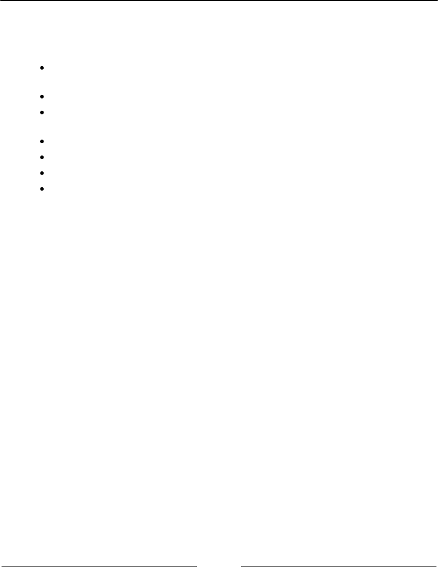
Machine Learning Chapter 4

[ 250 ]

Even in the case of CatBoost, the list of parameters is incredibly large, though well-detailed,

at https:/󰜌/󰜌tech.󰜌yandex.󰜌com/󰜌catboost/󰜌doc/󰜌dg/󰜌concepts/󰜌python-󰜌reference_󰜌catboost-

docpage/󰜌. For simple applications, you just have to tune the following key parameters:

one_hot_max_size : The threshold over which to target encode any categorical

variable

iterations : The number of iterations

od_wait: The number of iterations to wait if the evaluation metric doesn’t

improve

learning_rate: The learning rate

depth: The depth of trees

l2_leaf_reg: The regularization coefficient

random_strength and bagging_temperature to control the randomized

bagging

We start by importing all the necessary packages and functions:

Since CatBoost excels when dealing with categorical variables, we have to1.

rebuild the Forest Covertype dataset, because all its categorical variables have

already been one-hot-encoded. We therefore simply rebuild them and recreate

the dataset:

In: import numpy as np

from sklearn.datasets import fetch_covtype

from catboost import CatBoostClassifier, Pool

covertype_dataset = fetch_covtype(random_state=101,

shuffle=True)

label = covertype_dataset.target.astype(int) - 1

wilderness_area =

np.argmax(covertype_dataset.data[:,10:(10+4)],

axis=1)

soil_type = np.argmax(

covertype_dataset.data[:,(10+4):(10+4+40)],

axis=1)

data = (covertype_dataset.data[:,:10],

wilderness_area.reshape(-1,1),

soil_type.reshape(-1,1))

data = np.hstack(data)

Machine Learning Chapter 4

[ 251 ]

After creating it, we select the train, validation, and test portions as we did2.

before:

In: covertype_train = Pool(data[:15000,:],

label[:15000], [10, 11])

covertype_val = Pool(data[15000:20000,:],

label[15000:20000], [10, 11])

covertype_test = Pool(data[20000:25000,:],

None, [10, 11])

covertype_test_y = label[20000:25000]

It is time now to set the CatBoostClassifier. We decide on a low learning rate3.

(0.05) and a high number of iterations, a maximum tree depth of 8 (the actual

maximum for CatBoost is 16), optimize for MultiClass (log-loss) but monitor

accuracy both on the training and validation set:

In: model = CatBoostClassifier(iterations=4000,

learning_rate=0.05,

depth=8,

custom_loss = 'Accuracy',

eval_metric = 'Accuracy',

use_best_model=True,

loss_function='MultiClass')

We then start training, setting verbosity off but allowing a visual representation4.

of the training and its results, both in-sample and, more importantly, out-of-

sample:

In: model.fit(covertype_train, eval_set=covertype_val,

verbose=False, plot=True)

Here is an example of what visualization you can get for the model trained on the

CoverType dataset:

Machine Learning Chapter 4

[ 252 ]

After training, we simply predict the class and its associated probability:5.

In: preds_class = model.predict(covertype_test)

preds_proba = model.predict_proba(covertype_test)

An accuracy evaluation points out that the results are equivalent to XGBoost6.

(0.847 against 848) and the confusion matrix looks much cleaner, pointing out a

better classification job done by this algorithm:

In: from sklearn.metrics import accuracy_score, confusion_matrix

print('test accuracy:', accuracy_score(covertype_test_y,

preds_class))

print(confusion_matrix(covertype_test_y, preds_class))

Out: test accuracy: 0.847

[[1482 320 0 0 0 0 18]

[ 213 2199 12 0 10 12 2]

[ 0 13 260 5 0 23 0]

[ 0 0 6 18 0 3 0]

[ 2 40 5 0 30 0 0]

[ 0 16 33 1 0 94 0]

[ 31 0 0 0 0 0 152]]

Machine Learning Chapter 4

[ 253 ]

Dealing with big data

Big data puts data science projects under four points of view: volume (data quantity),

velocity, variety, and veracity (is your data really representing what it should be or is it

affected by some bias, distortion, or error?). The Scikit-learn package offers a range of

classes and functions that will help you effectively work with data so large that it cannot

entirely fit in the memory of a standard computer.

Before providing you with an overview of big data solutions, we have to create or import

some datasets in order to give you a better idea of the scalability and performances of

different algorithms. This will require about 1.5 gigabytes of your hard disk, which will be

let free after the experiment.

(Not big data in itself—nowadays, it is hard to find computers with less than 4 GB of

memory—yet, not even a toy dataset, it should provide you some idea).

Creating some big datasets as examples

As a typical example of big data analysis, we will use some textual data from the internet,

and we will take advantage of the available fetch_20newsgroups, which contains data of

11,314 posts, each one averaging about 206 words, which appeared in 20 different

newsgroups:

In: import numpy as np

from sklearn.datasets import fetch_20newsgroups

newsgroups_dataset = fetch_20newsgroups(shuffle=True,

remove=('headers', 'footers', 'quotes'),

random_state=6)

print ('Posts inside the data: %s' % np.shape(newsgroups_dataset.data))

print ('Average number of words for post: %0.0f' %

np.mean([len(text.split(' ')) for text in

newsgroups_dataset.data]))

Out: Posts inside the data: 11314

Average number of words for post: 206

Machine Learning Chapter 4

[ 254 ]

Instead, to work out a generic classification example, we will create three synthetic datasets

that contain from 100,000 to 10 million cases. You can create and use any of them according

to your computer's resources. We will always refer to the largest one for our experiments:

In: from sklearn.datasets import make_classification

X,y = make_classification(n_samples=10**5, n_features=5,

n_informative=3, random_state=101)

D = np.c_[y,X]

np.savetxt('large_dataset_10__5.csv', D, delimiter=",")

# the saved file should be around 14,6 MB

del(D, X, y)

X,y = make_classification(n_samples=10**6, n_features=5,

n_informative=3, random_state=101)

D = np.c_[y,X]

np.savetxt('large_dataset_10__6.csv', D, delimiter=",")

# the saved file should be around 146 MB

del(D, X, y)

X,y = make_classification(n_samples=10**7, n_features=5,

n_informative=3, random_state=101)

D = np.c_[y,X]

np.savetxt('large_dataset_10__7.csv', D, delimiter=",")

#the saved file should be around 1,46 GB

del(D, X, y)

After creating and using any of the datasets, you can remove them from disk by the

following command:

In: import os

os.remove('large_dataset_10__5.csv')

os.remove('large_dataset_10__6.csv')

os.remove('large_dataset_10__7.csv')

Scalability with volume

The trick to managing high volumes of data without loading too many megabytes (or

gigabytes) of data into your memory is to incrementally update the parameters of your

algorithm using only part of the examples at a time, repeating the update on the following

data chunks until all the observations have been elaborated at least once by the machine

learner.

This is possible in Scikit-learn thanks to the .partial_fit() method, which has been

made available to a certain number of supervised and unsupervised algorithms. By using

the .partial_fit() method and providing some basic information (for example, for

classification, you should know beforehand the number of classes to be predicted), you can

immediately start fitting your model even if you have a single case or a few observations.

Machine Learning Chapter 4

[ 255 ]

This method is called incremental learning. The chunks of data that you incrementally

fed into the learning algorithm are called batches. The critical points of incremental

learning are as follows:

Batch size

Data preprocessing

Number of passes with the same examples

Validation and parameters fine-tuning

Batch size generally depends on your available memory. The principle is that the larger the

data chunks the better, since the data sample will get more representatives of the data

distributions as its size grows. In addition, data preprocessing is challenging. Incremental

learning algorithms work well with data in the range of [-1,+1] or [0,+1] (for instance,

Multinomial Bayes won't accept negative values). However, to scale into such a precise

range, you need to know beforehand the range of each variable. Alternatively, you have to

do one of these: pass all the data once, record the minimum and maximum values, or

derive them from the first batch, trimming the following observations that exceed the initial

maximum and minimum values.

A more robust way to cope with this problem is to use a sigmoid

normalization that bounds all of the range of possible values between 0

and 1.

The number of passes can become a problem. In fact, as you pass the same examples

multiple times, you help the predictive coefficients converge to an optimum solution. If you

pass too many of the same observations, the algorithm will tend to overfit; that is, it will

adapt too much to the data repeated too many times. Some algorithms, such as the SGD

family, are also very sensitive to the order that you propose to the examples to be learned.

Therefore, you have to either set their shuffle option (shuffle=True) or shuffle the file rows

before the learning starts, keeping in mind that, for efficacy, the order of the rows proposed

for the learning should be casual.

Validation is a stream of batches, which can be achieved in two ways:

Validate in a progressive way; that is, test first how the model predicts newly

arrived data chunks before passing them to training.

Hold out some observations from every chunk. The latter is also the best way to

reserve a sample for grid search or some other optimization.

Machine Learning Chapter 4

[ 256 ]

In our example, we entrust the SGDClassifier with a log loss (analogous to a logistic

regression) to learn how to predict a binary outcome given 10**7 observations:

In: from sklearn.linear_model import SGDClassifier

from sklearn.preprocessing import MinMaxScaler

import pandas as pd

streaming = pd.read_csv('large_dataset_10__7.csv',

header=None, chunksize=10000)

learner = SGDClassifier(loss='log', max_iter=100)

minmax_scaler = MinMaxScaler(feature_range=(0, 1))

cumulative_accuracy = list()

for n,chunk in enumerate(streaming):

if n == 0:

minmax_scaler.fit(chunk.iloc[:,1:].values)

X = minmax_scaler.transform(chunk.iloc[:,1:].values)

X[X>1] = 1

X[X<0] = 0

y = chunk.iloc[:,0]

if n > 8:

cumulative_accuracy.append(learner.score(X,y))

learner.partial_fit(X,y,classes=np.unique(y))

print ('Progressive validation mean accuracy %0.3f' %

np.mean(cumulative_accuracy))

Out: Progressive validation mean accuracy 0.660

First, pandas read_csv allows us to iterate over the file by reading batches of 10,000

observations (the number can be increased or decreased according to your computing

resources).

We use the MinMaxScaler in order to record the range of each variable on the first batch.

For the following batches, we will use the rule that if it exceeds one of the limits of [0,+1],

they are trimmed to the nearest limit. Otherwise, we can use the partial_fit method of

the MinMaxScaler and learn the boundaries of the features as we learn with our model. The

only caveat to be considered when using the MinMaxScaler though is attention to outliers

because they can compress the numeric transformation to a portion of the [0, +1] interval.

Eventually, starting from the tenth batch, we will record the accuracy of the learning

algorithm on each newly received batch before using it to update the training. In the end,

the accumulated accuracy scores are averaged, offering a global performance estimation.

Machine Learning Chapter 4

[ 257 ]

Keeping up with velocity

Various algorithms work using incremental learning. For classification, we will recall the

following:

sklearn.naive_bayes.MultinomialNB

sklearn.naive_bayes.BernoulliNB

sklearn.linear_model.Perceptron

sklearn.linear_model.SGDClassifier

sklearn.linear_model.PassiveAggressiveClassifier

For regression, we will recall the following:

sklearn.linear_model.SGDRegressor

sklearn.linear_model.PassiveAggressiveRegressor

As for velocity, they are all comparable in speed. You can try for yourself with the

following script:

In: from sklearn.naive_bayes import MultinomialNB

from sklearn.naive_bayes import BernoulliNB

from sklearn.linear_model import Perceptron

from sklearn.linear_model import SGDClassifier

from sklearn.linear_model import PassiveAggressiveClassifier

import pandas as pd

from datetime import datetime

classifiers = {'SGDClassifier hinge loss' : SGDClassifier(loss='hinge',

random_state=101, max_iter=10),

'SGDClassifier log loss' : SGDClassifier(loss='log',

random_state=101, max_iter=10),

'Perceptron' : Perceptron(random_state=101,max_iter=10),

'BernoulliNB' : BernoulliNB(),

'PassiveAggressiveClassifier' : PassiveAggressiveClassifier(

random_state=101, max_iter=10)

}

large_dataset = 'large_dataset_10__6.csv'

for algorithm in classifiers:

start = datetime.now()

minmax_scaler = MinMaxScaler(feature_range=(0, 1))

streaming = pd.read_csv(large_dataset, header=None, chunksize=100)

learner = classifiers[algorithm]

cumulative_accuracy = list()

for n,chunk in enumerate(streaming):

y = chunk.iloc[:,0]

X = chunk.iloc[:,1:]

Machine Learning Chapter 4

[ 258 ]

if n > 50 :

cumulative_accuracy.append(learner.score(X,y))

learner.partial_fit(X,y,classes=np.unique(y))

elapsed_time = datetime.now() - start

print (algorithm + ' : mean accuracy %0.3f in %s secs'

% (np.mean(cumulative_accuracy),elapsed_time.total_seconds()))

Out: BernoulliNB : mean accuracy 0.734 in 41.101 secs

Perceptron : mean accuracy 0.616 in 37.479 secs

SGDClassifier hinge loss : mean accuracy 0.712 in 38.43 secs

SGDClassifier log loss : mean accuracy 0.716 in 39.618 secs

PassiveAggressiveClassifier : mean accuracy 0.625 in 40.622 secs

As a general note, remember that smaller batches are slower, since that

implies more disk access from a database or a file, which is always a

bottleneck.

Dealing with variety

Variety is another typical characteristic of big data. This is especially true when we are

dealing with textual data or very large categorical variables (for example, variables storing

website names in programmatic advertising). As you learn from batches of examples and as

you unfold categories or words, you will see that each one is an appropriate and exclusive

variable. You may find it difficult to handle the challenge of variety and the

unpredictability of large streams of data. Scikit-learn provides you with a simple and fast

way to implement the hashing trick and completely forget the problem of defining in

advance of a rigid variable structure.

The hashing trick uses hash functions and sparse matrices in order to save your time,

resources, and hassle. The hash functions are functions that map in a deterministic way any

input they receive. It doesn't matter if you feed them with numbers or strings, they will

always provide you with an integer number in a certain range. Sparse matrices are, instead,

arrays that record only values that are not zero, since their default value is zero for any

combination of their row and column. Therefore, the hashing trick bounds every possible

input; it doesn't matter if it was previously unseen to a certain range or position on a

corresponding input sparse matrix, which is loaded with a value that is not 0.

Machine Learning Chapter 4

[ 259 ]

Apart from the in-built hash function in Python, there are quite a few hashing algorithms

available in packages such as hashlib (https:/󰜌/󰜌docs.󰜌python.󰜌org/󰜌2/󰜌library/󰜌hashlib.

html). Interestingly, the hash function is also heavily used by Scikit-learn in many functions

and methods, and the MurmurHash 32 (https:/󰜌/󰜌github.󰜌com/󰜌aappleby/󰜌smhasher) is

available for you to use. It can be found among the utilities for developers (http:/󰜌/󰜌Scikit-

learn.󰜌org/󰜌stable/󰜌developers/󰜌utilities.󰜌html); just import it and use it straight out of

the box:

In: from sklearn.utils import murmurhash3_32

print (murmurhash3_32("something", seed=0, positive=True))

For instance, if your input is Python, a hashing command such as abs(hash('Python'))

can transform that into the integer number 539294296 and then assign the value of 1 to the

cell at the 539294296 column index. The hash function is a very fast and convenient way to

invariably locate the same column index given the same input. The use of only absolute

values ensures that each index corresponds only to a column in our array (negative indexes

just start from the last column, and hence in Python, each column of an array can be

expressed by both a positive and negative number).

The example that follows uses the HashingVectorizer class, a convenient class that

automatically takes documents, separates the words, and transforms them, thanks to the

hashing trick, into an input matrix. The script aims at learning why posts are published in

20 distinct newsgroups based on the words used on the existing posts in the newsgroups:

In: import pandas as pd

from sklearn.linear_model import SGDClassifier

from sklearn.feature_extraction.text import HashingVectorizer

def streaming():

for response, item in zip(newsgroups_dataset.target,

newsgroups_dataset.data):

yield response, item

hashing_trick = HashingVectorizer(stop_words='english', norm = 'l2')

learner = SGDClassifier(random_state=101, max_iter=10)

texts = list()

targets = list()

for n, (target, text) in enumerate(streaming()):

texts.append(text)

targets.append(target)

if n % 1000 == 0 and n >0:

learning_chunk = hashing_trick.transform(texts)

if n > 1000:

last_validation_score = learner.score(learning_chunk, targets),

learner.partial_fit(learning_chunk, targets,

classes=[k for k in range(20)])

texts, targets = list(), list()

Machine Learning Chapter 4

[ 260 ]

print ('Last validation score: %0.3f' % last_validation_score)

Out: Last validation score: 0.710

At this point, no matter what text you may input, the predictive algorithm will always

answer by pointing out a class. In our case, it points out a newsgroup suitable for the post

to appear on it. Let's try out this algorithm with a text taken from a classified ad:

In: New_text = ["A 2014 red Toyota Prius v Five with fewer than 14K" +

"miles. Powered by a reliable 1.8L four cylinder " +

"hybrid engine that averages 44mpg in the city and " +

"40mpg on the highway."]

text_vector = hashing_trick.transform(New_text)

print (np.shape(text_vector), type(text_vector))

print ('Predicted newsgroup: %s' %

newsgroups_dataset.target_names[learner.predict(text_vector)])

Out: (1, 1048576) <class 'scipy.sparse.csr.csr_matrix'>

Predicted newsgroup: rec.autos

Naturally, you may change the New_text variable and discover where your text most

likely will be displayed in a newsgroup. Note that the HashingVectorizer class has

transformed the text into a csr_matrix (which is quite an efficient sparse matrix) to save

memory, having a dataset of about one million columns.

An overview of Stochastic Gradient Descent

(SGD)

We will complete this part of the chapter devoted to learning from big data with a quick

overview of the SGD family, comprising SGDClassifier (for classification) and

SGDRegressor (for regression).

Like other classifiers, they can be fit by using the .fit() method (passing row by row the

in-memory dataset to the learning algorithm) or the previously seen .partial_fit()

method based on batches. In the latter case, if you are classifying, you have to declare the

predicted classes with the class parameter. It can accept a list containing all the class code

that it should expect to meet during the training phase.

SGDClassifier can behave as a logistic regression when the loss parameter is set to loss. It

transforms into a linear SVC if the loss is set to hinge. It can also take the form of other loss

functions, or even the loss functions working for regression.

Machine Learning Chapter 4

[ 261 ]

SGDRegressor mimics a linear regression using the squared_loss loss parameter. Instead,

the Huber loss transforms the squared loss into a linear loss over a certain distance epsilon

(another parameter to be fixed). It can also act as a linear SVR using the

epsilon_insensitive loss function or the slightly different

squared_epsilon_insensitive (which penalizes outliers more).

As in other situations with machine learning, the performance of the different loss functions

on your data science problem cannot be estimated a priori. Anyway, please take into

account that if you are doing classification and you need an estimation of class

probabilities, you will be limited in your choice to log or modified_huber only.

The key parameters that require tuning for this algorithm to work best with your data are

as follows:

n_iter: The number of iterations over the data. As a rule of thumb, the more the

passes, the better the optimization of the algorithm. However, there is a higher

risk of overfitting if the passes are too many. Empirically, SGD tends to converge

to a stable solution after having seen 10**6 examples. Given your examples, set

your number of iterations accordingly.

penalty: You have to choose l1, l2, or elasticnet, which are all different

regularization strategies, to avoid overfitting because of overparameterization

(using too many unnecessary parameters leads to the memorization of

observations more than the learning of patterns). Briefly, l1 tends to reduce

unhelpful coefficients to zero, l2 just attenuates them, and elasticnet is a mix of l1

and l2 strategies.

alpha: This is a multiplier of the regularization term; the higher the alpha, the

more the regularization. We advise you to find the best alpha value by

performing a grid search ranging from 10**-7 to 10**-1.

l1_ratio: The l1 ratio is used for elasticnet penalty. The suggested value or 0.15

will usually prove quite effective.

learning_rate: This sets how much the coefficients are affected by every single

example. Usually, it is optimal for classifiers and invscaling for regression. If

you want to use invscaling for classification, you'll have to set eta0 and

power_t (invscaling = eta0 / (t**power_t)). With invscaling, you

can start with a lower learning rate, which is less than the optimal rate, though it

will decrease slower.

epsilon: This should be used if your loss is huber, epsilon_insensitive, or

squared_epsilon_insensitive.

shuffle: If this is True, the algorithm will shuffle the order of the training data

in order to improve the generalization of the learning.

Machine Learning Chapter 4

[ 262 ]

A peek into natural language processing

(NLP)

This section is not strictly related to machine learning, but it contains some machine

learning results in the area of natural language processing. Python has many packages to

process text data, and one of most powerful and complete toolkit for text processing is

NLTK, the Natural Language Tool Kit.

Other NLP toolkits available for the Python community are gensim

(https:/󰜌/󰜌radimrehurek.󰜌com/󰜌gensim/󰜌) and spaCy (https:/󰜌/󰜌spacy.󰜌io/󰜌)

In the following sections, we'll explore NLTK core functionalities. We will work on the

English language; for other languages, you will first need to download the language

corpora (note that sometimes languages have no free open source corpora for NLTK).

Please refer to the official website of NLTK data, http:/󰜌/󰜌www.󰜌nltk.󰜌org/󰜌nltk_󰜌data/󰜌, to

have access to corpora and lexical resources in many languages, ready to work with NLTK.

Word tokenization

Tokenization is the act of splitting the text into words. Chunking whitespace seems very

easy, but it's not, because the text contains punctuation and contractions. Let's start with an

example:

In: my_text = "The coolest job in the next 10 years will be " +\

"statisticians. People think I'm joking, but " +\

"who would've guessed that computer engineers " +\

"would've been the coolest job of the 1990s?"

simple_tokens = my_text.split(' ')

print (simple_tokens)

Out: ['The', 'coolest', 'job', 'in', 'the', 'next', '10', 'years', 'will',

'be', 'statisticians.', 'People', 'think', "I'm", 'joking,', 'but',

'who', "would've", 'guessed', 'that', 'computer', 'engineers',

"would've", 'been', 'the', 'coolest', 'job', 'of', 'the', '1990s?']

Machine Learning Chapter 4

[ 263 ]

Here, you can immediately see that something is wrong. The following tokens contain more

than a word: statisticians. (with the final period), I'm (two words), would've, and

1990s? (with the final question mark). Let's now see how NLTK performs better in this

task (of course, under the hood, the algorithm is more complex than a simple whitespace

chunker):

In: import nltk

nltk_tokens = nltk.word_tokenize(my_text)

print (nltk_tokens)

Out: ['The', 'coolest', 'job', 'in', 'the', 'next', '10', 'years',

'will', 'be', 'statisticians', '.', 'People', 'think', 'I',

"'m", 'joking', ',', 'but', 'who', 'would', "'ve", 'guessed',

'that', 'computer', 'engineers', 'would', "'ve", 'been', 'the',

'coolest', 'job', 'of', 'the', '1990s', '?']

While executing this or some other NLTK package calls, in case of an error

saying "Resource u'tokenizers/punkt/english.pickle' not

found.", just type nltk.download() on your console and select to either

download everything or browse for the missing resource that triggered

the warning.

Here, the quality is better, and each token is associated with a word in the text.

Note that ., ,, and ? are tokens, too.

There also exists a sentence tokenizer (see the nltk.tokenize.punkt module), but it's

seldom used in data science.

Also, beyond the general-purpose English tokenizer, NLTK contains many other tokenizers

to be used in different contexts. For example, if you're working on tweets, TweetTokenizer

can be extremely useful to parse tweet-like documents. The most useful options are to

remove handles, shorten consecutive characters, and properly tokenize hashtags. Here's an

example:

In: from nltk.tokenize import TweetTokenizer

tt = TweetTokenizer(strip_handles=True, reduce_len=True)

tweet = '@mate: I loooooooove this city!!!!!!! #love #foreverhere'

tt.tokenize(tweet)

Out: [':', 'I', 'looove', 'this', 'city', '!', '!', '!', '#love',

'#foreverhere']

Machine Learning Chapter 4

[ 264 ]

Stemming

Stemming is the action of reducing inflectional forms of words and taking the words to

their core concepts. For example, the concept behind is, be, are, and am is the same.

Similarly, the concept behind go and goes, as well as table and tables, is the same. The

operation of deriving the root concept for each word is called stemming. In NLTK, you can

choose the stemmer that you'd like to use (there are several ways to get the root part of

words). We'll show you one of them, letting the others in Jupyter Notebook associated with

this part of the book:

In: from nltk.stem import *

stemmer = LancasterStemmer()

print ([stemmer.stem(word) for word in nltk_tokens])

Out: ['the', 'coolest', 'job', 'in', 'the', 'next', '10', 'year',

'wil', 'be', 'stat', '.', 'peopl', 'think', 'i', "'m", 'jok',

',', 'but', 'who', 'would', "'ve", 'guess', 'that', 'comput',

'engin', 'would', "'ve", 'been', 'the', 'coolest', 'job',

'of', 'the', '1990s', '?']

In the example, we used the Lancaster stemmer, which is one of the most powerful and

recent algorithms. Checking the result, you will immediately see that it's all lowercase and

statistician is associated with its root, stat. Good job!

Word tagging

Tagging, or POS-Tagging, is the association between a word (or a token) and its part-of-

speech tag (POS-Tag). After tagging, you know what (and where) the verbs, adjectives,

nouns, and so on, are in the sentence. Even in this case, NLTK makes this complex

operation very easy:

In: import nltk

print (nltk.pos_tag(nltk_tokens))

Out: [('The', 'DT'), ('coolest', 'NN'), ('job', 'NN'), ('in', 'IN'),

('the', 'DT'), ('next', 'JJ'), ('10', 'CD'), ('years', 'NNS'),

('will', 'MD'), ('be', 'VB'), ('statisticians', 'NNS'), ('.', '.'),

('People', 'NNS'), ('think', 'VBP'), ('I', 'PRP'), ("'m", 'VBP'),

('joking', 'VBG'), (',', ','), ('but', 'CC'), ('who', 'WP'),

('would', 'MD'), ("'ve", 'VB'), ('guessed', 'VBN'), ('that', 'IN'),

('computer', 'NN'), ('engineers', 'NNS'), ('would', 'MD'),

("'ve", 'VB'), ('been', 'VBN'), ('the', 'DT'), ('coolest', 'NN'),

('job', 'NN'), ('of', 'IN'), ('the', 'DT'), ('1990s', 'CD'),

('?', '.')]

Machine Learning Chapter 4

[ 265 ]

Using the syntax of NLTK, you will realize that the The token represents a determiner (DT),

coolest and job represent nouns (NN), in represents a conjunction, and so on. The

association is really detailed; in the case of a verb, there are six possible tags, as follows:

Take: VB (verb, base form)

Took: VBD (verb, past tense)

Taking: VBG (verb, gerund)

Taken: VBN (verb, past participle)

Take: VBP (verb, singular present tense)

Takes: VBZ (verb, third-person singular present tense)

If you need a more detailed view of the sentence, you may want to use the parse tree tagger

to understand its syntactic structure. This operation is rarely used in data science, since it's

great for sentence-by-sentence analysis.

Named entity recognition (NER)

The goal of NER is to recognize tokens associated with people, organizations, and locations.

Let's use an example to explain it further:

In: import nltk

text = "Elvis Aaron Presley was an American singer and actor. Born in \

Tupelo, Mississippi, when Presley was 13 years old he and his \

family relocated to Memphis, Tennessee."

chunks = nltk.ne_chunk(nltk.pos_tag(nltk.word_tokenize(text)))

print (chunks)

Out: (S

(PERSON Elvis/NNP)

(PERSON Aaron/NNP Presley/NNP)

was/VBD

an/DT

(GPE American/JJ)

singer/NN

and/CC

actor/NN

./.

Born/NNP

in/IN

(GPE Tupelo/NNP)

,/,

(GPE Mississippi/NNP)

,/,

Machine Learning Chapter 4

[ 266 ]

when/WRB

(PERSON Presley/NNP)

was/VBD

13/CD

years/NNS

old/JJ

he/PRP

and/CC

his/PRP$

family/NN

relocated/VBD

to/TO

(GPE Memphis/NNP)

,/,

(GPE Tennessee/NNP)

./.)

An extract of the Wikipedia page on Elvis is analyzed and NER-processed. A few entities

that have been recognized by NER are listed here:

Elvis Aaron Presley: PERSON

American: GPE (Geopolitical entity)

Tupelo, Mississippi: GPE (Geopolitical entity)

Memphis, Tennessee: GPE (Geopolitical entity)

Stopwords

Stopwords are the least informative pieces (or tokens) in text, since they are the most

common words (such as the, it, is, as, and not). Stopwords are often removed. And, exactly

the way it happens in the feature selection phase if you remove them, the processing takes

less time and less memory; also, it is sometimes more accurate. Removing stopwords

decreases the overall entropy of the text, thereby making whatever signal is in there more

apparent and easier to represent in features.

A list of English stopwords is available in Scikit-learn, too. For the stopwords in other

languages, check out NLTK:

In: from sklearn.feature_extraction import text

stop_words = text.ENGLISH_STOP_WORDS

print (stop_words)

Out: frozenset(['all', 'six', 'less', 'being', 'indeed', 'over', 'move',

'anyway', 'four', 'not', 'own', 'through', 'yourselves',

'fify', 'where', 'mill', 'only', 'find', 'before', 'one',

Machine Learning Chapter 4

[ 267 ]

'whose', 'system', 'how', ...

In: from nltk.corpus import stopwords

print(stopwords.words('english'))

Out: ['i', 'me', 'my', 'myself', 'we', 'our', 'ours', 'ourselves',

'you', 'your', 'yours', 'yourself', 'yourselves', 'he', 'him',

'his', 'himself', 'she', 'her', 'hers', 'herself', 'it', 'its',

'itself', 'they', 'them', 'their', 'theirs', 'themselves', 'what',

'which', 'who', 'whom', 'this', 'that', 'these', '...

In: print(stopwords.words('german'))

Out: ['aber', 'alle', 'allem', 'allen', 'aller', 'alles', 'als', 'also',

'am', 'an', 'ander', 'andere', 'anderem', 'anderen', 'anderer',

'anderes', 'anderm', 'andern', 'anderr', 'anders', 'auch',

'auf', 'au', ...

A complete data science example – text

classification

Now, here's a complete example that allows you to put each text in the right category. We

will use the 20newsgroup dataset, which was already introduced in Chapter 1, First Steps.

To make things more realistic and prevent the classifier from overfitting the data, we'll

remove email headers, footers (such as a signature), and quotes. In addition, in this case,

the goal is to classify between two similar categories: sci.med and sci.space. We will use

the accuracy measure to evaluate the classification:

In: import nltk

from sklearn.datasets import fetch_20newsgroups

from sklearn.feature_extraction.text import TfidfVectorizer

from sklearn.linear_model import SGDClassifier

from sklearn.metrics import accuracy_score

from sklearn.datasets import fetch_20newsgroups

import numpy as np

categories = ['sci.med', 'sci.space']

to_remove = ('headers', 'footers', 'quotes')

twenty_sci_news_train = fetch_20newsgroups(subset='train',

remove=to_remove, categories=categories)

twenty_sci_news_test = fetch_20newsgroups(subset='test',

remove=to_remove, categories=categories)

Machine Learning Chapter 4

[ 268 ]

Let's start with the easiest approach to preprocess the textual data-using TfIdf. Remember

that Tfidf is the multiplication of the frequency of the word within the document, by the

inverse of its frequency across all the documents. High scores indicate that the word is used

multiple times in the current document, but it's rare in the others (that is, it's a keyword of

the document):

In: tf_vect = TfidfVectorizer()

X_train = tf_vect.fit_transform(twenty_sci_news_train.data)

X_test = tf_vect.transform(twenty_sci_news_test.data)

y_train = twenty_sci_news_train.target

y_test = twenty_sci_news_test.target

Now let's use a linear classifier (SGDClassifier) to perform the classification task. One last

thing to do is to print out the classification accuracy:

In: clf = SGDClassifier()

clf.fit(X_train, y_train)

y_pred = clf.predict(X_test)

print ("Accuracy=", accuracy_score(y_test, y_pred))

Out: Accuracy= 0.878481012658

An accuracy of 87.8 percent is a very good result. The entire program consists of less than

20 lines of code. Now, let's see if we can get something better. In this chapter, we've learned

stopword removal, tokenization, and stemming. Let's see whether we gain accuracy by

using them:

In: def clean_and_stem_text(text):

tokens = nltk.word_tokenize(text.lower())

clean_tokens = [word for word in tokens if word not in stop_words]

stem_tokens = [stemmer.stem(token) for token in clean_tokens]

return " ".join(stem_tokens)

cleaned_docs_train = [clean_and_stem_text(text) for text in

twenty_sci_news_train.data]

cleaned_docs_test = [clean_and_stem_text(text) for text in

twenty_sci_news_test.data]

Machine Learning Chapter 4

[ 269 ]

The clean_and_stem_text function basically lowercases, tokenizes, stems, and

reconstructs every document in the dataset. Finally, we will apply the same preprocessing

(Tfidf) and classifier (SGDClassifier) that we used in the preceding example:

In: X1_train = tf_vect.fit_transform(cleaned_docs_train)

X1_test = tf_vect.transform(cleaned_docs_test)

clf.fit(X1_train, y_train)

y1_pred = clf.predict(X1_test)

print ("Accuracy=", accuracy_score(y_test, y1_pred))

Out: Accuracy= 0.893670886076

This processing requires more time, but we gained an accuracy of about 1.5 percent. An

accurate tuning of the parameters of Tfidf and a cross-validated choice of the parameters

of the classifier will eventually boost the accuracy to over 90 percent. So far, we're happy

with this performance, but you can try to break that barrier.

An overview of unsupervised learning

In all the methods we've seen so far, every sample or observation has its own target label or

value. In some other cases, the dataset is unlabeled and, to extract the structure of the data,

you need an unsupervised approach. In this section, we're going to introduce two methods

to perform clustering, as they are among the most used methods for unsupervised learning.

It is useful to bear in mind that often the terms clustering and unsupervised

learning are considered synonymous, though, actually, unsupervised

learning has a larger meaning.

K-means

The first method that we'll introduce is named K-means, the most commonly used

clustering algorithm despite its inevitable shortcomings. In signal processing, K-means is

the equivalent of a vectorial quantization, that is, the selection of the best codeword (from a

given codebook) that better approximates the input observation (or a word).

Machine Learning Chapter 4

[ 270 ]

You must provide the algorithm with the K parameter, which is the number of clusters.

Sometimes, this might be a limitation because you have to investigate first which is the

right K for the current dataset.

K-means iterates an EM (expectation/maximization) approach. During the first phase, it

assigns each training point to the closest cluster centroid; during the second phase, it moves

the cluster centroid to the center of mass of the points assigned to it (to reduce distortion).

The initial placement of centroids is random. Consequently, you may need to run the

algorithm several times so as not to find a local minimum.

That's all for the theory behind the algorithm; now, let's see it in practice. In this section,

we're using two two-dimensional dummy datasets that will explain what's going on better.

Both datasets are composed of 2,000 samples so that you can also have an idea about the

processing time.

Now, let's create the artificial datasets, and then let's represent them by a plot:

In: %matplotlib inline

import numpy as np

import matplotlib.pyplot as plt

from sklearn import datasets

N_samples = 2000

dataset_1 = np.array(datasets.make_circles(n_samples=N_samples,

noise=0.05, factor=0.3)[0])

dataset_2 = np.array(datasets.make_blobs(n_samples=N_samples,

centers=4, cluster_std=0.4, random_state=0)

plt.scatter(dataset_1[:,0], dataset_1[:,1], c=labels_1,

alpha=0.8, s=64, edgecolors='white')

plt.show()

Machine Learning Chapter 4

[ 271 ]

This is the first dataset we created, made of concentric rings of points (a quite tricky

problem because the represented clusters are non spherical):

In: plt.scatter(dataset_2[:,0], dataset_2[:,1], alpha=0.8, s=64,

c='blue', edgecolors='white')

plt.show()

Here is the second one, made of separated bubbles of points:

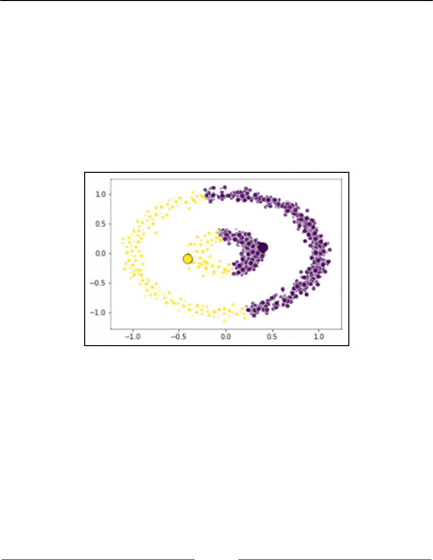
Machine Learning Chapter 4

[ 272 ]

Now it's time to apply K-means. We will set K=2 in this case. Let's see the results:

In: from sklearn.cluster import KMeans

K_dataset_1 = 2

km_1 = KMeans(n_clusters=K_dataset_1)

labels_1 = km_1.fit(dataset1).labels

plt.scatter(dataset_1[:,0], dataset_1[:,1], c=labels_1,

alpha=0.8, s=64, edgecolors='white')

plt.scatter(km_1.cluster_centers_[:,0], km_1.cluster_centers_[:,1],

s=200, c=np.unique(labels_1), edgecolors='black')

plt.show()

This is the result with obtain on this problem:

As you can see, K-means is not performing very well on this dataset, because it expects

spherical-shaped data clusters. For this dataset, a Kernel-PCA should be applied before

using K-means.

Now let's see how it performs on a spherical-clustered data. In this case, based on our

knowledge of the problem and the silhouette coefficient, we will set K=4:

In: K_dataset_2 = 4

km_2 = KMeans(n_clusters=K_dataset_2)

labels_2 = km_2.fit(dataset2).labels

plt.scatter(dataset_2[:,0], dataset_2[:,1], c=labels_2,

alpha=0.8, s=64, edgecolors='white')

plt.scatter(km_2.cluster_centers_[:,0], km_2.cluster_centers_[:,1],

marker='s', s=100, c=np.unique(labels_2), edgecolors='black')

plt.show()

Machine Learning Chapter 4

[ 273 ]

The results we get on this problem are much better:

As expected, the plotted result is great. The centroids and clusters are exactly what we had

in mind while looking at the unlabeled dataset. Now we are going to check if there is any

other cluster approach that could help us solve the clustering problem when our clusters

are non-spherical.

In real-world cases, you may consider using the Silhouette Coefficient to

have an idea about how well-defined the clusters are. It is an evaluation

metric of consistency within groups, applicable to various clustering

results, and even class structures in supervised learning. You can read

more about Silhouette Coefficient at

http://Scikit-learn.org/stable/modules/clustering.html#silhouett

e-coefficient.

DBSCAN – a density-based clustering technique

Now we will introduce you to DBSCAN, a density-based clustering technique. It's a very

simple technique. It selects a random point; if the point is in a dense area (if it has more

than N neighbors do), it starts growing the cluster, including all the neighbors, and the

neighbors of the neighbors, until it reaches a point where there are no more neighbors.

Machine Learning Chapter 4

[ 274 ]

If the point is not in a dense area, it is classified as noise. Then, another unlabeled point is

selected randomly and the process starts over. This technique is great for non-spherical

clusters, but it works equally well with spherical ones. The input is just the neighborhood

radius (the eps parameter, that is, the maximum distance between two points that are

being considered neighbors), and the output is the cluster membership label for each point.

Note that the points labeled by the value-1 are classified as noise by

DBSCAN.

Let's see an example on the dataset we had previously introduced:

In: from sklearn.cluster import DBSCAN

dbs_1 = DBSCAN(eps=0.25)

labels_1 = dbs_1.fit(dataset1).labels

plt.scatter(dataset_1[:,0], dataset_1[:,1], c=labels_1,

alpha=0.8, s=64, edgecolors='white')

plt.show()

Now the clusters are correctly located by the DBSCAN algorithm:

The result is perfect now. No points have been classified as noise (only the

and 1 labels

appear in the label set):

In: np.unique(labels_1)

Out: array([0, 1])

Machine Learning Chapter 4

[ 275 ]

Now let's move on to the other dataset:

In: dbs_2 = DBSCAN(eps=0.5)

labels_2 = dbs_2.fit(dataset2).labels

plt.scatter(dataset_2[:,0], dataset_2[:,1], c=labels_2,

alpha=0.8, s=64, edgecolors='white')

plt.show()

In: np.unique(labels_2)

Out: array([-1, 0, 1, 2, 3])

It took some time to select the best settings for DBSCAN, and in this case, four clusters have

been detected and a few points have been classified as noise (since the label set contains -1):

At the end of this section, a last important note is that in this essential

introduction of K-means and DBSCAN, we have always used the

Euclidean distance, as it is the default distance metric in these functions

(though other distance metrics can also be used if you find them

appropriate). When using this distance in real cases, remember that you

have to normalize each feature (z-normalization) so that every feature

contributes equally to the final distortion. If the dataset is not normalized,

the features that have larger support will have more decision power on

the output label, and that's something that we don't want.

Machine Learning Chapter 4

[ 276 ]

Latent Dirichlet Allocation (LDA)

For text, instead, a popular unsupervised algorithm that can be used to understand a

common set of words in a collection of documents is Latent Dirichlet Allocation or LDA.

Note that another algorithm, the Linear Discriminant Analysis, also has

the same acronym, but the two algorithms are completely unconnected.

LDA aims to extract sets of homogeneous words, or topics, out of a collection of

documents. The math behind the algorithm is very advanced; here we will see just a

practical notion of it.

Let's start with an example to explain why LDA is popular and why other unsupervised

methods aren't good enough when dealing with text. K-means and DBSCAN, for example,

provide a hard decision for each sample, putting each point in a disjoint partition.

Documents, instead, often describe covering topics together (think about Shakespeare's

books; they're a good mix of tragedy, romance, and adventure). On text documents, any

hard decision would be almost certainly wrong. LDA, instead, provides as output a mixture

of topics composing the document, along with an indication of how much the topic is

represented in the document.

Let's use an example to explain how it works. We will train the algorithm on two

categories; cars and medicine, from the 20-newsgroup dataset (we have already used the

same dataset before in the chapter, in the earlier paragraph, Preparing tools and datasets):

In: import nltk

Import gensim

from sklearn.datasets import fetch_20newsgroups

def tokenize(text):

return [token.lower() \

for token in gensim.utils.simple_preprocess(text) \

if token not in gensim.parsing.preprocessing.STOPWORDS]

text_dataset=fetch_20newsgroups(categories=['rec.autos','sci.med'],

random_state=101,

remove=('headers', 'footers', 'quotes'))

documents = text_dataset.data

print("Document count:", len(documents))

Out: Document count: 1188

Machine Learning Chapter 4

[ 277 ]

Each one of the 1,188 documents composing the dataset is a string. For example, the first

document contains the following text:

In: documents[0]

Out: 'nI have a new doctor who gave me a prescription today for something

called nSeptra DS. He said it may cause GI problems and I have a

sensitive stomach nto begin with. Anybody ever taken this antibiotic.

Any good? Suggestions nfor avoiding an upset stomach? Other tips?n'

This document is definitely about medicine; there is nothing really important anyway for

the algorithm. Now let's tokenize and create a dictionary of all the words included in the

dataset. Mind that the tokenization operation also removes the stopwords and puts each

word in lowercase:

In: processed_docs = [tokenize(doc) for doc in documents]

word_dic = gensim.corpora.Dictionary(processed_docs)

print("Num tokens:", len(word_dic))

Out: Num tokens: 16161

In the dataset, there are just over 16,000 distinct words. It's now time to filter too common

words and too rare ones. In this step, we will keep the words appearing at least 10 times

and no more than in 20% of the documents. At this point, we have the "Bag Of Words" (or

BoW) representation of each document; that is, each document is represented as a

dictionary containing how many times each word appears in the text. The absolute position

of each word in the text is lost, exactly as if you put all the words of the document in a bag.

As a result, not all of the signal in the text is captured in the features based on this

approach, but most of the time, it suffices to make an effective model:

In: word_dic.filter_extremes(no_below=10, no_above=0.2)

bow = [word_dic.doc2bow(doc) for doc in processed_docs]

Finally, here's the core class for LDA. In this example, we instruct LDA that in the dataset

there are just two topics. We also provide other parameters to make the algorithm converge

(if not, you'll receive a warning from the Python interpreter). Note that this algorithm

works on many CPUs on your computer to speed up the process. If it doesn't work, please

use the mono-process class, gensim.models.ldamodel.LdaModel, with the same

parameters:

In: lda_model = gensim.models.LdaMulticore(bow, num_topics=2,

id2word=word_dic, passes=10,

iterations=500)

Machine Learning Chapter 4

[ 278 ]

Finally, after a couple of minutes, the model is trained. To see the association between

words and topics, run the following code:

In: lda_model.print_topics(-1)

Out: [(0, '0.011*edu + 0.008*com + 0.007*health + 0.007*medical +

0.007*new + 0.007*use + 0.006*people + 0.005*time +

0.005*years + 0.005*patients'), (1, '0.018*car + 0.008*good +

0.008*think + 0.008*cars + 0.007*msg + 0.006*time +

0.006*people + 0.006*water + 0.005*food + 0.005*engine')]

As you can see, the algorithm went through all the documents and learned that the main

topics are cars and medicine. Note that the algorithm doesn't provide a short name for the

topics, but their composition (the numbers are the weights of each word inside each topic,

ranked from highest to lowest). In addition, note that some words appear in both topics;

they are ambiguous words that can be used in both senses.

Finally, let's see how the algorithm works on an unseen document. To make things easier,

let's create a sentence that contains both topics, for example I've shown the doctor my new car.

He loved its big wheels! Then, after having created a Bag-of-Words representation of this new

document, LDA will produce two scores, one for each topic:

In: new_doc = "I've shown the doctor my new car. He loved its big wheels!"

bow_doc = word_dic.doc2bow(tokenize(new_doc))

for index, score in sorted(lda_model[bow_doc], key=lambda tup:

-1*tup[1]):

print("Score: {}t Topic: {}".format(score,

lda_model.print_topic(index, 5)))

Out: Score: 0.5047402389474193 Topic: 0.011*edu + 0.008*com +

0.007*health + 0.007*medical + 0.007*new

Score: 0.49525976105258074 Topic: 0.018*car + 0.008*good +

0.008*think + 0.008*cars + 0.007*msg

The scores for both the topics are around 0.5 and 0.5, meaning that the sentence contains a

good balance of the subjects car and medicine. What we've shown here is just an example

of two topics; but the same implementation, thanks to the performing library Gensim, can

also allocate process the whole English Wikipedia in a matter of few hours.

Machine Learning Chapter 4

[ 279 ]

A different approach than LDA is provided by the Word2Vec algorithm, a very recent

model for embedding words in vectors. Compared to LDA, Word2Vec keeps track of the

position of the words in a sentence, and this additional context helps to disambiguate some

words better. Word2Vec is trained using a deep-learning-like approach, but the

implementation provided by the Gensim library makes it very easy to train and use. Note

that while LDA aims to understand the topics in a document, Word2Vec works at the word

level and tries to understand what the semantic relationship between words in a low-

dimensionality space is (that is, creating an n-dimensional vector for each word). Let's see

an example, to make things clear.

We will use the movie review dataset to train the Word2Vec model. The training is done

simply by passing the sentences composing the corpora to the Word2Vec constructor, and,

eventually, the number of workers that can work in parallel on the training task:

In: from gensim.models import Word2Vec

from nltk.corpus import movie_reviews

w2v = Word2Vec(movie_reviews.sents(), workers=4)

w2v.init_sims(replace=True)

The last line of code simply freezes the model, not allowing any additional updates. This

also brings an additional and very welcome benefit: reducing the memory fingerprint of the

object.

Visualizing vectors that represent the words may be complicated; therefore, let's see some

similarities (that is, similar vectors in the low-dimensional subspace). Here, we will ask the

model to provide the top five most similar words (along with the similarity score) to the

words house and countryside. This is just an example; it's possible to retrieve similar

words for all words contained in the input corpora:

In: w2v.wv.most_similar('house', topn=5)

Out: [('apartment', 0.8799251317977905),

('body', 0.8719735145568848),

('hotel', 0.8618944883346558),

('head', 0.848749041557312),

('boat', 0.8469674587249756)]

In: w2v.vw.most_similar('countryside', topn=5)

Out: [('motorcycle', 0.9531803131103516),

('marches', 0.9499938488006592),

('rural', 0.9467764496803284),

('shuttle', 0.9466159343719482),

('mining', 0.9461280107498169)]

Machine Learning Chapter 4

[ 280 ]

How is Word2Vec able to do so? Simply, with a similarity score in the low-dimensionality

vector space. In fact, to see the vector representation of each word, perform the following:

In: w2v.wv['countryside']

Out: array([-0.09412272, 0.07695948, -0.14981066, 0.04894404,

-0.03712097, -0.17099065, -0.0379245 , -0.05336253,

0.06084964, -0.01273731, -0.03949985, -0.06456301,

-0.03289359, -0.06889232, 0.02217194, ...

The array is composed of 100 dimensions; you can increase or decrease it by setting the

size parameter while training the model. 100 is the default value.

In the most_similar method we've previously used, you can also specify the negative

words to use (that is, to subtract similar words). A classic example is finding a similar word

to woman and king without queen. The top result is, unsurprisingly, man:

In: w2v.wv.most_similar(positive=['woman', 'king'], negative=['queen'],

topn=3)

Out: [('man', 0.8440324068069458),

('girl', 0.7671926021575928),

('child', 0.7635241746902466)]

The model, thanks to the vector representation, also provides the method to identify the

non-matching words in a set of similar words; that is, the word that doesn't match the

context (in this case, the context is the bedroom):

In: w2v.wv.doesnt_match(['bed', 'pillow', 'cake', 'mattress'])

Out: 'cake'

Finally, all the preceding methods are built on similarity scores. The model also provides

the raw score of similarity between words; here's an example of the similarity score of

woman and girl and woman and boy. The first similarity is higher, though the second is not

zero, since both words are connected by the fact we're talking about people:

In: w2v.wv.similarity('woman', 'girl'), w2v.similarity('woman', 'boy')

Out: (0.90198267746062233, 0.82372486297773828)

Machine Learning Chapter 4

[ 281 ]

Summary

In this chapter, we introduced the essentials of machine learning. We started with some

easy, but still quite effective, classifiers (linear and logistic regressors, Naive Bayes, and K-

Nearest Neighbors). Then, we moved on to the more advanced ones (SVM). We explained

how to compose weak classifiers together (ensembles, Random Forests, Gradient Tree

Boosting) and touched on three awesome gradient-boosted classifiers: XGboost, LightGBM,

and CatBoost. Finally, we had a peek at the algorithms used in big data, clustering, and

NLP.

In the next chapter, we are going to introduce you to the basics of visualization with

Matplotlib, how to operate EDA with pandas and achieve beautiful visualizations with

Seaborn, and how to set up a web server to provide information on demand.

Visualization, Insights, and

Results

After exploring machine learning, but not because the topic is less relevant than others, we

are going to illustrate how to create visualizations with Python to enrich your data science

project. Visualization plays an important role in helping you communicate the results and

insights derived from data and the learning process.

In this chapter, you will learn how to do the following:

Use the basic pyplot functions from the matplotlib package

Leverage a pandas DataFrame for Explorative Data Analysis (EDA)

Create beautiful and interactive charts with Seaborn

Visualize the machine learning and optimization processes we discussed

in Chapter 3, The Data Pipeline, and Chapter 4, Machine Learning

Understand and visually communicate variables' importance and their

relationship with the target outcome

Set up a prediction server that uses HTTP to accept and provide predictions as a

service

Introducing the basics of matplotlib

Visualization is a fundamental aspect of data science, allowing data scientists to better and

more effectively communicate their findings to the organization they operate in, to both

data experts and non-experts. Providing the nuts and bolts of the principles behind

communicating information and crafting engaging beautiful visualizations is beyond the

scope of our book, but we can recommend suitable resources if you want to improve your

skills.

Visualization, Insights, and Results Chapter 5

[ 283 ]

For basic visualization rules, you can visit https:/󰜌/󰜌lifehacker.󰜌com/󰜌5909501/󰜌how-󰜌to-

choose-󰜌the-󰜌best-󰜌chart-󰜌for-󰜌your-󰜌data. We also recommend the books of Prof. Edward

Tufte on analytic design and visualization.

We can instead provide a fast and to-the-point series of essential recipes that can get you

started on visualization using Python, and that you can refer to anytime you need to create

a specific graphics chart. Consider all the snippets of code as your visualization building

blocks; you can arrange them with different configurations and features just by using the

large choice of parameters that we are going to present to you.

matplotlib is a Python package for plotting graphics. Created by John Hunter, it has been

developed in order to address a lack of integration between Python and external software

with graphical capabilities, such as MATLAB or gnuplot. Greatly influenced by MATLAB's

way of operating and functions, matplotlib presents a quite similar syntax. In particular,

the matplotlib.pyplot module, perfectly compatible with MATLAB, will be the core of

our essential introduction to all the indispensable graphical tools to represent your data

and analysis. MATLAB is indeed a standard for visualization in the data analysis and

scientific community because of its recognized capabilities when it comes to exploratory

analysis, mainly due to its smooth and easy to use plotting functions.

Each pyplot command makes a change on an initially instantiated figure. Once you set a

figure, all additional commands will operate on it. Thus, it is easy to incrementally improve

and enrich your graphic representation. In order for you to take advantage of the code and

be able to personalize it to your needs, all the following examples are presented together

with commented building blocks so that you can later draft your basic representation, and

then look through this chapter for specific parameters among the examples in order to

improve your chart as you planned it.

With the pyplot.figure() command, you can initialize a new visualization, though it

suffices to call a plotting command to automatically start it. Instead, by using

pyplot.show(), you close the figure that you were operating on, and you can open and

operate on new figures.

Before starting with a few visualization examples, let's import the necessary packages in

order to run all the examples:

In: import numpy as np

import matplotlib.pyplot as plt

import matplotlib as mpl

In this way, we can always refer to pyplot, the MATLAB-like module, as plt, and access

the complete matplotlib functionality set with the help of mpl.

Visualization, Insights, and Results Chapter 5

[ 284 ]

If you are using a Jupyter Notebook (or Jupyter Lab), you can use this line

magic: %matplotlib inline. After writing the command in a cell of the

notebook and running it, you can have your plots drawn directly on the

notebook itself, instead of having the graphics presented in a separate

window (by default, the GUI backend of matplotlib is the TkAgg

backend). If you prefer a different backend such as Qt (www.qt.io), which

is often distributed with Python scientific distributions, you just have to

run this line magic instead: %matplotlib Qt.

Trying curve plotting

Our first problem will require you to draw a function with pyplot. Drawing a function is

quite straightforward; you just have to get a series of x coordinates and map them to the y

axis by using the function that you want to plot. Since the mapping results are stored away

into two vectors, the plot function will deal with the curve representation. The precision of

the representation will be greater if the mapped points are enough (50 points is a good

sampling number):

In: import numpy as np

import matplotlib.pyplot as plt

x = np.linspace(0, 5, 50)

y_cos = np.cos(x)

y_sin = np.sin(x)

Using the NumPy linspace() function, we will create a series of 50 equally distanced

numbers ranging from 0 to 5. We can use them to map our y to the cosine and sine

functions:

In: plt.figure() # initialize a figure

plt.plot(x,y_cos) # plot series of coordinates as a line

plt.plot(x,y_sin)

plt.xlabel('x') # adds label to x axis

plt.ylabel('y') # adds label to y axis

plt.title('title') # adds a title

plt.show() # close a figure

Visualization, Insights, and Results Chapter 5

[ 285 ]

Here is your first plot:

The pyplot.plot command can plot more curves in a sequence, with each curve taking a

different color according to an internal color schema, which can be customized by

explicating the favored color sequence. To do so, you have to manipulate the list containing

the sequence of colors that matplotlib uses:

In: list(mpl.rcParams['axes.prop_cycle'])

Out: [{'color': '#1f77b4'},

{'color': '#ff7f0e'},

{'color': '#2ca02c'},

{'color': '#d62728'},

{'color': '#9467bd'},

{'color': '#8c564b'},

{'color': '#e377c2'},

{'color': '#7f7f7f'},

{'color': '#bcbd22'},

{'color': '#17becf'}]

#1f77b4, #ff7f0e, #2ca02c, and all the others are all colors expressed in

hexadecimal form. In order to figure out how they look, you can use the

colorhexa website, providing you with useful information on each of

them: https:/󰜌/󰜌www.󰜌colorhexa.󰜌com/󰜌.

Visualization, Insights, and Results Chapter 5

[ 286 ]

The hack can be done by using the cycler function and feeding it with a list of string

names referring to the colors you want to use in sequence:

In: mpl.rcParams['axes.prop_cycle'] = mpl.cycler('color',

['blue', 'red', 'green'])

Moreover, the plot command, if not given any other information, will assume that you are

going to plot a line. Therefore, it will link all the provided points in a curve. If you add a

new parameter such as '.' – that is, plt.plot(x,y_cos,'.') – you signal that you

instead want to plot a series of separated points (the string for a line is '-', but we will

soon show another example).

In this way, if you've customized rcParams['axes.prop_cycle'] as proposed

previously, the next graphs will first have a blue curve, then the second will be red, and the

third green. Then, the color loop will restart. We leave this decision to you. All the

examples in this chapter will just follow the standard color sequence, but you are free to

experiment with better color settings.

Please note that you can also set the title of the graph and label the axis by the title, xlabel,

and ylabel from pyplot.

Using panels for clearer representations

Our second example will demonstrate to you how to create multiple graphics panels and

plot a representation on each of them. We will also try to personalize the drawn curves by

using different colors, sizes, and styles. Here is the example:

In: import matplotlib.pyplot as plt

# defines 1 row 2 column panel, activates figure 1

plt.subplot(1,2,1)

plt.plot(x,y_cos,'r--')

# adds a title

plt.title('cos')

# defines 1 row 2 column panel, activates figure 2

plt.subplot(1,2,2)

plt.plot(x,y_sin,'b-')

plt.title('sin')

plt.show()

Visualization, Insights, and Results Chapter 5

[ 287 ]

The plot displays the cosine and sine curves on two distinct graphic panels:

The subplot command accepts the subplot(nrows, ncols, plot_number) parameter

form. Therefore, when instantiated, it reserves a certain amount of space for the

representation based on the nrows and ncols parameters and number of plots on the

plot_number area (starting from area 1 on the left).

You can also accompany the plot command coordinates with another string parameter,

which is useful for the definition of color and the type of the represented curve. The strings

work by combining the codes that you can find on the following links:

https:/󰜌/󰜌matplotlib.󰜌org/󰜌api/󰜌lines_󰜌api.󰜌html#matplotlib.󰜌lines.󰜌Line2D.󰜌set_

linestyle: Will present the different line styles.

http://matplotlib.org/api/colors_api.html: Offers a complete overview of

the basic built-in colors. The page also points out that you can either use the

color parameter together with the HTML names or hex strings for colors, or

define the color you desire by using an RGB tuple, where each value of the tuple

lies in the range of [0,1]. For instance, a valid parameter is color =

(0.1,0.9,0.9), which will create a color made of 10% red, 90% green, and 90%

blue.

http://matplotlib.org/api/markers_api.html: Lists all the possible marker

styles you can adopt for your points.

Visualization, Insights, and Results Chapter 5

[ 288 ]

Plotting scatterplots for relationships in data

Scatterplots plot two variables as points on a plane, and they can help you figure out the

relationship between the two variables. They are also quite effective if you want to

represent groups and clusters. In our example, we will create three data clusters and

represent them in a scatterplot with different shapes and colors:

In: from sklearn.datasets import make_blobs

import matplotlib.pyplot as plt

D = make_blobs(n_samples=100, n_features=2,

centers=3, random_state=7)

groups = D[1]

coordinates = D[0]

Since we have to plot three different groups, we will have to use three distinct plot

commands. Each command specifies a different color and shape (the 'ys', 'm*', 'rD'

strings, where the first letter is the color and the second is the marker). Please also note that

each plot instance is marked by a label parameter, which is used to assign a name to the

group that has to be reported later in a legend:

In: plt.plot(coordinates[groups==0,0],

coordinates[groups==0,1],

'ys', label='group 0') # yellow square

plt.plot(coordinates[groups==1,0],

coordinates[groups==1,1],

'm*', label='group 1') # magenta stars

plt.plot(coordinates[groups==2,0],

coordinates[groups==2,1],

'rD', label='group 2') # red diamonds

plt.ylim(-2,10) # redefines the limits of y axis

plt.yticks([10,6,2,-2]) # redefines y axis ticks

plt.xticks([-15,-5,5,-15]) # redefines x axis ticks

plt.grid() # adds a grid

plt.annotate('Squares', (-12,2.5)) # prints text at coordinates

plt.annotate('Stars', (0,6))

plt.annotate('Diamonds', (10,3))

plt.legend(loc='lower left', numpoints= 1)

# places a legend of labelled items

plt.show()

Visualization, Insights, and Results Chapter 5

[ 289 ]

The resulting plot will be a scatterplot of the three groups accompanied by their respective

labels:

We have also added a legend (pyplot.legend), fixed a limit for both the axes

(pyplot.xlim and pyplot ylim), and precisely explicated the ticks (plt.xticks and

plt.yticks) that had to be put on them by specifying a list of values. Therefore, the grid

(pyplot.grid) divides the plot exactly into nine quadrants and allows you to have a better

idea of where the groups are positioned. Finally, we printed some text pointing out the

group names (pyplot.annotate).

Histograms

Histograms can effectively represent the distribution of a variable. Here, we will visualize

two normal distributions, both characterized by unit standard deviation, one having a

mean of

and the other a mean of 3.0:

In: import numpy as np

import matplotlib.pyplot as plt

x = np.random.normal(loc=0.0, scale=1.0, size=500)

z = np.random.normal(loc=3.0, scale=1.0, size=500)

plt.hist(np.column_stack((x,z)),

bins=20,

histtype='bar',

color = ['c','b'],

stacked=True)

plt.grid()

plt.show()

Visualization, Insights, and Results Chapter 5

[ 290 ]

The conjoint distributions can offer a different insight on the data if there is a classification

problem:

There are a few ways to personalize this kind of plot and obtain further insights about the

analyzed distributions. First, by changing the number of bins, you will change how the

distributions are discretized (discretization is the process that transforms continuous

functions or series of values into a reduced, countable set of numbers:

en.wikipedia.org/wiki/Discretization). Generally, 10 to 20 bins offer a good

understanding of the distribution, though it really depends on the size of the dataset as well

as the distribution. For instance, the Freedman-Diaconis rule prescribes that the optimal

number of bins in a histogram in order to meaningfully visualize your data depends on the

bin's width, to be calculated using the interquartile range (IQR) and the number of

observations:

Having calculated h, which is the bin width, the number of bins is computed by dividing

the difference between the maximum and the minimum value by h:

bins=(max-min) / h

Visualization, Insights, and Results Chapter 5

[ 291 ]

We can also change the type of visualization from bars to steps by changing the parameters

from histtype='bar' to histtype='step'. By changing the stacked Boolean

parameter to False, the curves won't stack into a unique bar in the parts that overlap, but

you will clearly see the separate bars of each one.

Bar graphs

Bar graphs are useful for comparing quantities in different categories. They can be arranged

either horizontally or vertically to present the mean estimate and error bands. They can be

used to present various statistics of your predictors and how they relate to the target

variable.

In our example, we will present the mean and standard deviation for the four variables of

the Iris dataset:

In: from sklearn.datasets import load_iris

import numpy as np

import matplotlib.pyplot as plt

iris = load_iris()

average = np.mean(iris.data, axis=0)

std = np.std(iris.data, axis=0)

range_ = range(np.shape(iris.data)[1])

In our representation, we will prepare two subplots: one with horizontal bars (plt.barh),

and the other with vertical bars (plt.bar). The standard error is represented by an error

bar, and according to the graph orientation, we can use the xerr parameter for horizontal

bars and yerr for vertical ones:

In: plt.subplot(1,2,1) # defines 1 row, 2 columns panel, activates figure 1

plt.title('Horizontal bars')

plt.barh(range_,average, color="r",

xerr=std, alpha=0.4, align="center")

plt.yticks(range_, iris.feature_names)

plt.subplot(1,2,2) # defines 1 row 2 column panel, activates figure 2

plt.title('Vertical bars')

plt.bar(range_,average, color="b", yerr=std, alpha=0.4, align="center")

plt.xticks(range_, range_)

plt.show()

Visualization, Insights, and Results Chapter 5

[ 292 ]

Horizontal and verticals bars are now together in the same plot:

It is important to note the use of the plt.xticks command (and of plt.yticks for the

ordinate axis). The first parameter informs the command about the number of ticks that

have to be placed on the axis, and the second one explicates the labels that have to be put

on the ticks.

Another interesting parameter to notice is alpha, which has been used to set the

transparency level of the bar. The alpha parameter is a float number ranging from 0.0, fully

transparent, to 1.0, which causes the color to be shown in different levels of opaqueness.

Image visualization

The last possible visualization that we explore using matplotlib has to do with images.

Resorting to plt.imgshow is useful when you are working with image data. Let's take as

an example the Olivetti dataset, an open source set of images of 40 people who provided 10

images of themselves at different times (and with different expressions, a fact that makes it

more challenging for testing face recognition algorithms). The images from this dataset are

provided as feature vectors of pixel intensities. Therefore, it is important to reshape the

vectors in order to make them resemble a matrix of pixels. Setting the interpolation to

'nearest' helps to smooth the picture:

In: from sklearn.datasets import fetch_olivetti_faces

import numpy as np

Visualization, Insights, and Results Chapter 5

[ 293 ]

import matplotlib.pyplot as plt

dataset = fetch_olivetti_faces(shuffle=True, random_state=5)

photo = 1

for k in range(6):

plt.subplot(2, 3, k+1)

plt.imshow(dataset.data[k].reshape(64, 64),

cmap=plt.cm.gray,

interpolation='nearest')

plt.title('subject '+str(dataset.target[k]))

plt.axis('off')

plt.show()

A complete panel of images will be plotted:

We can also visualize handwritten digits or letters. In our example, we will plot the first

nine digits from the scikit-learn handwritten digit dataset and set the extent of both the axes

(by using the extent parameter and providing a list of minimum and maximum values) to

align the grid to the pixels:

In: from sklearn.datasets import load_digits

digits = load_digits()

for number in range(1,10):

fig = plt.subplot(3, 3, number)

fig.imshow(digits.images[number],

cmap='binary',

interpolation='none',

extent=[0,8,0,8])

Visualization, Insights, and Results Chapter 5

[ 294 ]

fig.set_xticks(np.arange(0, 9, 1))

fig.set_yticks(np.arange(0, 9, 1))

fig.grid()

plt.show()

A simple close-up on a single number can be obtained by printing only one image:

In: plt.imshow(digits.images[0],

cmap='binary',

interpolation='none',

extent=[0,8,0,8])

# Extent defines the images max and min

# of the horizontal and vertical values

plt.grid()

Visualization, Insights, and Results Chapter 5

[ 295 ]

The resulting image clearly highlights how pixels constitute the image and their gray levels:

Selected graphical examples with pandas

Using appropriately set hyper-parameters, many machine learning algorithms can

optimally learn how to map your data with respect to your target outcome. Yet, their

predictive performance can be improved further by fixing hidden and subtle problems in

data. It is not simply a matter of detecting any missing or outlying case. Sometimes, it is a

matter of whether there are any groups or unusual distributions in the data (for instance,

multimodal distributions). Clearly drafted data plots can explicate the relationship between

variables, and they can lead to the creation of new and better features in order to predict,

with increased accuracy, your target variable.

The just-described practice is called explorative data analysis (EDA), and it can bring

effective results if it is done accordingly with the following:

It should be fast, allowing you to explore and develop new ideas, and test them,

and restart with a new exploration and fresh ideas

It should be based on graphical representations in order to better describe data as

a whole, no matter how high its dimensionality is

Visualization, Insights, and Results Chapter 5

[ 296 ]

The pandas DataFrame offers many EDA tools that can help you in your explorations.

However, first you have to transform your data into a DataFrame:

In: import pandas as pd

print ('Your pandas version is: %s' % pd.__version__)

from sklearn.datasets import load_iris

iris = load_iris()

iris_df = pd.DataFrame(iris.data, columns=iris.feature_names)

groups = list(iris.target)

iris_df['groups'] = pd.Series([iris.target_names[k] for k in groups])

Out: Your pandas version is: 0.23.1

Please check your version of pandas. We tested the code in the book

under the version 0.23.1 of pandas, and it should also hold for the later

releases.

We will be using the iris_df DataFrame for all the examples presented in the following

paragraphs.

The pandas package actually relies on matplotlib functions for its visualizations. It simply

provides a convenient wrapper around the otherwise complex plotting instructions. This

offers advantages in terms of speed and simplicity, which are the core values of any EDA

process. Instead, if your purpose is to best communicate the findings by using beautiful

visualization, you may notice that it is not so easy to customize the pandas graphical

outputs. Therefore, when it is paramount to create specific graphics outputs, it is better to

start working directly from scratch using matplotlib instructions.

Working with boxplots and histograms

Distributions should always be the first aspect to be inspected in your data. Boxplots draft

the key figures in the distribution and help you spot outliers. Just use the boxplot method

on your DataFrame for a quick overview:

In: boxplots = iris_df.boxplot(return_type='axes')

Visualization, Insights, and Results Chapter 5

[ 297 ]

Here are the boxplots of all the numeric variables of the dataset:

If you already have groups in your data (from categorical variables, or derived from

unsupervised learning), just point out the variable you need data to be represented in the

boxplot and specify that you need to have it separated by the groups (use the by parameter

followed by the string name of the grouping variable):

In: boxplots = iris_df.boxplot(column='sepal length (cm)',

by='groups',

return_type='axes')

After running the code, you will get the boxplot by groups:

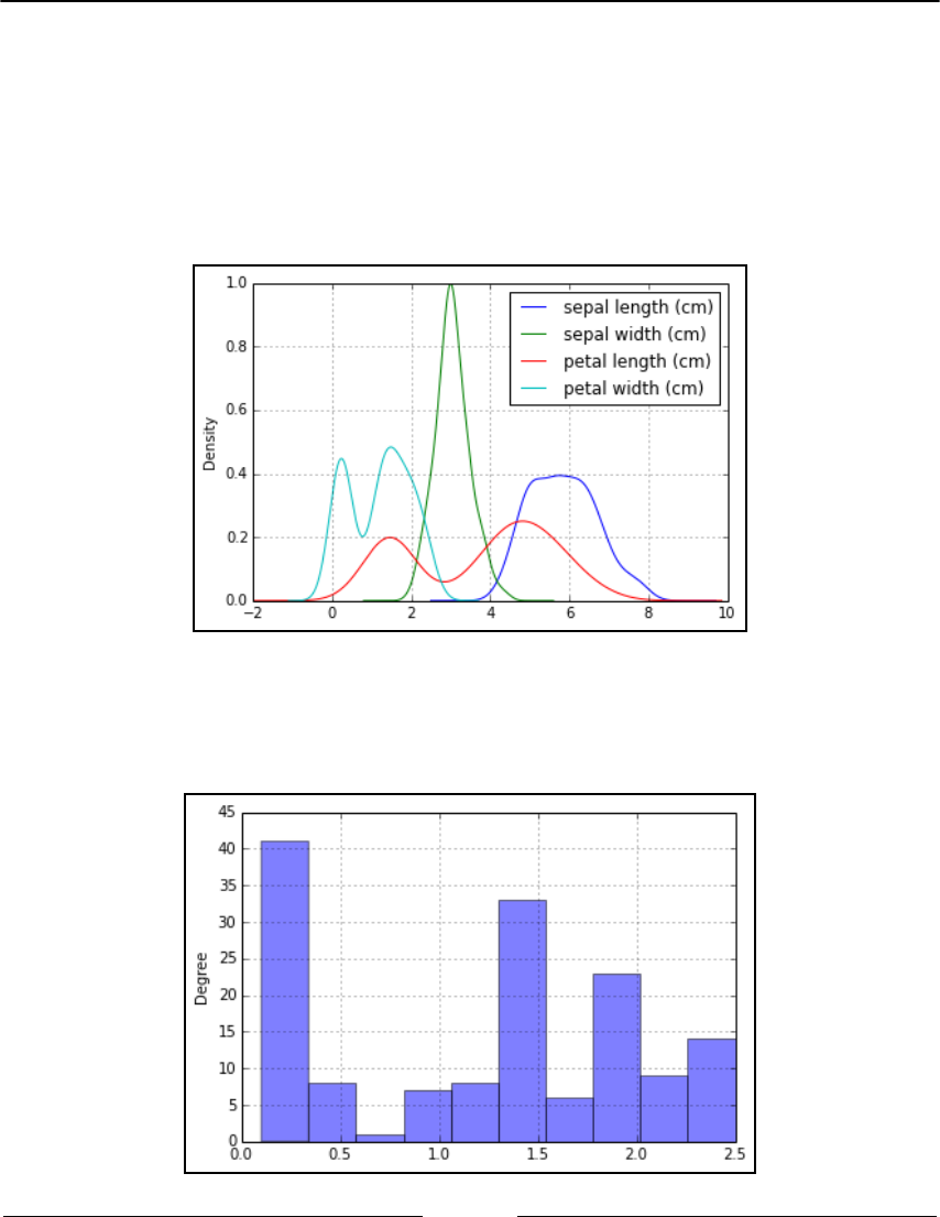
Visualization, Insights, and Results Chapter 5

[ 298 ]

In this way, you can quickly know whether the variable is a good discriminator of the

group differences. Anyway, boxplots cannot provide you with a complete view of

distributions as histograms and density plots. For instance, by using histograms and

density plots, you can figure out whether there are distribution peaks or valleys:

In: densityplot = iris_df.plot(kind='density')

The code prints the distributions for all the numeric variables of the dataset:

In: single_distribution = iris_df['petal width (cm)'].plot(kind='hist',

alpha=0.5)

Here is the resulting distribution represented by a histogram:

Visualization, Insights, and Results Chapter 5

[ 299 ]

You can obtain both histograms and density plots by using the plot method. This method

allows you to represent the whole dataset, specific groups of variables (you just have to

provide a list of the string names and do some fancy indexing), or even single variables.

Plotting scatterplots

Scatterplots can be used to effectively understand whether the variables are in a nonlinear

relationship, and you can get an idea about their best possible transformations to achieve

linearization. If you are using an algorithm based on linear combinations, such as linear or

logistic regression, figuring out how to render their relationship more linearly will help you

achieve a better predictive power:

In: colors_palette = {0: 'red', 1: 'yellow', 2:'blue'}

colors = [colors_palette[c] for c in groups]

simple_scatterplot = iris_df.plot(kind='scatter', x=0, y=1, c=colors)

After running the code, a nicely drawn scatterplot will appear:

Scatterplots can be turned into hexagonal binning plots. In addition, they help you

effectively visualize the point densities, where the points naturally aggregate together

more, thus revealing clusters hidden in your data. For achieving such results, you may use

some of the variables originally present in the dataset, or the dimensions obtained by a

PCA or by another dimensionality reduction algorithm:

In: hexbin = iris_df.plot(kind='hexbin', x=0, y=1, gridsize=10)

Visualization, Insights, and Results Chapter 5

[ 300 ]

Here is the resulting hexbin plot:

The gridsize parameter indicates how many data points the chart will summarize in a

single grid. A larger number will create large grid cells, whereas a smaller one will create

small cells.

Scatterplots are bivariate. Consequently, you'll require a single plot for every variable

combination. If your variables are not so many in number (otherwise, the visualization will

be cluttered), a quick solution is to use the pandas command to draw a matrix of

scatterplots automatically (using the kernel density estimation, 'kde', in order to plot the

distribution of each feature on the diagonal of the chart):

In: from pandas.plotting import scatter_matrix

colors_palette = {0: "red", 1: "green", 2: "blue"}

colors = [colors_palette[c] for c in groups]

matrix_of_scatterplots = scatter_matrix(iris_df,

alpha=0.2,

figsize=(6, 6),

color=colors,

diagonal='kde')

Visualization, Insights, and Results Chapter 5

[ 301 ]

After running the previous code, you will get a complete matrix of plots (densities on the

diagonal):

A few parameters can control various aspects of the scatterplot matrix. The alpha

parameter controls the amount of transparency, and figsize provides the width and

height of the matrix in inches. Finally, color accepts a list indicating the color of each point

in the plot, thus allowing the depicting of different groups in data. In addition, by selecting

'kde' or 'hist' on your diagonal parameter, you can opt to represent density curves or

histograms of each variable on the diagonal of the scatter matrix.

Visualization, Insights, and Results Chapter 5

[ 302 ]

Discovering patterns by parallel coordinates

The scatterplot matrix can inform you about the conjoint distributions of your features. It

helps you locate groups in data and verify whether they are distinguishable. Parallel

coordinates are another kind of plot that is helpful in providing you with a hint about the

most group-discriminating variables present in your data.

By plotting all the observations as parallel lines with respect to all the possible variables

(arbitrarily aligned on the abscissa), parallel coordinates will help you spot whether there

are streams of observations grouped as your classes, and understand the variables that best

separate the streams (the most useful predictor variables). Naturally, in order for the chart

to be meaningful, the features in the plot should have the same scale (otherwise, normalize

them) as in the Iris dataset:

In: from pandas.tools.plotting import parallel_coordinates

pll = parallel_coordinates(iris_df,'groups')

The previous code will output the parallel coordinates:

parallel_coordinates is a pandas function that, in order to work properly, just needs as

parameters the data DataFrame and the string name of the variable containing the groups

whose separability you want to test. For this reason, you should have the group variable

available in your dataset. However, don't forget to remove it after you finish exploring by

using the DataFrame.drop('variable name', axis=1, inplace=True) method.

Visualization, Insights, and Results Chapter 5

[ 303 ]

Wrapping up matplotlib's commands

As we have seen in the previous paragraph, pandas can speed up exploring data visually

since it wraps up into single commands what would have required an entire code snippet

using matplotlib. The idea behind this is that unless you need to tailor and configure a

special visualization, using a wrapper can allow you to create standard graphics faster.

Apart from pandas, other packages assemble low-level instructions from matplotlib into

more user-friendly commands for specific representations and usage:

Seaborn is a package that extends your visualization capabilities by providing

you with a set of statistical plots useful for finding out trends and discriminating

groups

ggplot is a port of a popular R library, ggplot2 (ggplot2.tidyverse.org),

based on the visualization grammar proposed in Leland Wilkinson's book,

Grammar of Graphics. The R library is continuously developed and it offers

much functionality; the Python porting (ggplot.yhathq.com) features the basics

(ggplot.yhathq.com/docs/index.html) and its complete development is still

underway (github.com/yhat/ggplot).

MPLD3 (mpld3.github.io) leverages the JavaScript library for graphics

manipulation, D3.js, in order to easily transform any matplotlib output into

HTML code, which can be rendered using a browser and a tool such as a Jupyter

Notebook; or within an internet website.

Bokeh (bokeh.pydata.org/en/latest/) is an interactive visualization package

that leverages JavaScript and browser-rendered outputs. It is a great replacement

for D3.js since you just need Python in order to leverage the capabilities of

JavaScript to quickly represent your data in an interactive way.

In the following pages, we will introduce Seaborn, providing some building blocks for

leveraging their visualizations in your data science projects.

Visualization, Insights, and Results Chapter 5

[ 304 ]

Introducing Seaborn

Created by Michael Waskom and hosted on the PyData website

(http://seaborn.pydata.org/), Seaborn is a library that wraps up the low-level matplotlib

with the entire pyData stack, allowing integrating charts with data structures from NumPy

and pandas, and with statistical routines from SciPy and StatModels. All that is achieved

with a particular care to aesthetics, thanks to built-in themes, and to color palettes

especially devised to reveal patterns in data.

If you don't have Seaborn presently installed on your system (the Anaconda distributions

provide it by default, for instance), you can easily get it both by pip and conda (reminding

you that the conda version may lag behind the pip version taken directly from PyPI, the

Python Package Index.

$> pip install seaborn

$> conda install seaborn

In these examples, we have used version 0.9 of the Seaborn package.

You can upload the package and set the Seaborn style as the default matplotlib style by the

following:

In: import seaborn as sns

sns.set()

This is enough to turn all your matplotlib-based representations into more visually

appealing charts:

In: x = np.linspace(0, 5, 50)

y_cos = np.cos(x)

y_sin = np.sin(x)

plt.figure()

plt.plot(x,y_cos)

plt.plot(x,y_sin)

plt.xlabel('x')

plt.ylabel('y')

plt.title('sin/cos functions')

plt.show()

Visualization, Insights, and Results Chapter 5

[ 305 ]

Here is the result:

You can obtain interesting results from any of the previously seen charts, even the ones

generated using graphical methods in pandas (after all, pandas also relies on matplotlib for

creating its explorative plots).

There are five preset themes in Seaborn:

darkgrid

whitegrid

dark

white

ticks

Visualization, Insights, and Results Chapter 5

[ 306 ]

darkgrid is the default one. You can easily try each one by using the set_style

command and the name of your preferred theme, and then running your plot commands:

In: sns.set_style('whitegrid')

All you have to do is just decide which theme helps you better convey the information on

your chart. You can limit a style to a single representation enclosing it:

In: with sns.axes_style('whitegrid'):

# Your plot commands here

pass

Other stylish changes may involve the spines, which are the borders of the chart. Using the

despine command, you can easily remove the top and right borders:

In: sns.despine()

Moreover, you can remove the left border using the left=True parameter, offset the axis

using the offset parameter, and trim it (using trim=True). All these operations were

otherwise not so accessible because of matplotlib commands alone.

Another useful control that Seaborn permits you regards the scale of the chart. A certain

chart scale (involving different thickness of lines, size of fonts, and so on) is called a context,

and the available contexts are self-explicative-paper, notebook, talk, and poster as possible

options. For instance, if your chart has to be displayed on an MS PowerPoint presentation,

just run the following command before creating the graphics:

In: sns.set_context("talk")

Let's see an example of some of such stylish effects on our initial sin/cos chart:

In: sns.set_context("talk")

with sns.axes_style('whitegrid'):

plt.figure()

plt.plot(x,y_cos)

plt.plot(x,y_sin)

plt.show()

sns.set()

Visualization, Insights, and Results Chapter 5

[ 307 ]

The code will plot the following chart:

Also, choosing the right color cycle or set may help your graphical representation shine. For

this, Seaborn offers the color_palette() command, which won't just tell the current

palette's RBG values (if run with no parameters); it will also accept the name of any palette

offered by Seaborn or any matplotlib colormap. It even accepts custom lists of colors

provided by you in any matplotlib format (RGB tuples, hex color codes, or HTML color

names) in order to create your own palette:

In: current_palette = sns.color_palette()

print (current_palette)

sns.palplot(current_palette)

After running the code, you will visualize the current palette both in values and colors:

Visualization, Insights, and Results Chapter 5

[ 308 ]

There are a few palettes available, as mentioned. First, all Seaborn palettes are the

following:

deep

muted

bright

pastel

dark

colorblind

You also have to add hls, husl, and all the matplotlib colormaps, which can be reversed

by appending _r to their name, or made darker by appending _d.

Both the names and examples of matplotlib colormaps can be found at

this web page: http:/󰜌/󰜌matplotlib.󰜌org/󰜌examples/󰜌color/󰜌colormaps_

reference.󰜌html.

The hls color space is an automatic transformation in the RGB scale of values, which may

or may not work for your representations since colors have different intensities (for

instance, yellow and green colors are perceived as brighter whereas blue is perceived as

darker).

As an alternative to hsl, you can use the husl palette, which is friendlier for the human

eye, as explained by http://www.hsluv.org/.

Finally, you can just create a personalized palette using the Color Brewer tool, which can be

both found online (http:/󰜌/󰜌www.󰜌personal.󰜌psu.󰜌edu/󰜌cab38/󰜌ColorBrewer/󰜌ColorBrewer_

intro.󰜌html) or required in an app from your Jupyter Notebook. In a notebook cell, using

the choose_colorbrewer_palette command will make an interactive tool appear. For

everything to work, it is essential that you specify as a parameter the data_type, a string

explicating the nature of your palette related to the data you intend to represent:

Sequential if you want to represent continuity

Diverging for representing contrasts

Qualitative when you just want to discriminate between different classes

Let's see how to create a custom sequential palette, and use it:

In: your_palette = sns.choose_colorbrewer_palette('sequential')

Visualization, Insights, and Results Chapter 5

[ 309 ]

A complete dashboard will appear:

After setting the colors, your_palette will turn into a list of the RGB values:

In: print(your_palette)

Out:[(0.91109573770971852, 0.90574395025477683, 0.94832756940056306),

(0.7764706015586853, 0.77908498048782349, 0.88235294818878174),

(0.61776242186041452, 0.60213766261643054, 0.78345253116944269),

(0.47320263584454858, 0.43267974257469177, 0.69934642314910889),

(0.35681661753093497, 0.20525952297098493, 0.58569783322951374)]

When you are done with your choice, you can just call

sns.set_palette(your_palette) and have the colors used when drawing all your

charts.

If you need just to operate on a chart with some specific colors, using a with statement and

nesting the chart snippet under it will suffice, as we have seen for the themes before.

Instead, if you definitely need to set a certain palette, use set_palette.

The color palette is made up of six colors, helping you distinguish at least six trends or

classes. If you need to distinguish more, you simply can operate with the hls palette and

point out the number of colors you need to cycle:

In: new_palette=sns.color_palette('hls', 10)

sns.palplot(new_palette)

Here is the resulting palette:

Visualization, Insights, and Results Chapter 5

[ 310 ]

Finally, closing our section about themes and colors, since Seaborn is another, smarter way

to use functions offered by matplotlib, we remind you that the resulting charts can be

modified further using any basic command coming from matplotlib itself. Or, they can be

further transformed by packages such as MPLD3 or Bokeh into JavaScript.

Enhancing your EDA capabilities

Seaborn doesn't just make your charts more beautiful and easily controlled in their aspect;

it also provides you with new tools for EDA that helps you discover distributions and

relationships between variables.

Before proceeding, let's reload the package and have both the Iris and Boston datasets

ready in pandas DataFrame format:

In: import seaborn as sns

sns.set()

from sklearn.datasets import load_iris

iris = load_iris()

X_iris, y_iris = iris.data, iris.target

features_iris = [a[:-5].replace(' ','_') for a in iris.feature_names]

target_labels = {j: flower \

for j, flower in enumerate(iris.target_names)}

df_iris = pd.DataFrame(X_iris, columns=features_iris)

df_iris['target'] = [target_labels[y] for y in y_iris]

from sklearn.datasets import load_boston

boston = load_boston()

X_boston, y_boston = boston.data, boston.target

features_boston = np.array(['V'+'_'.join([str(b), a])

for a,b in zip(boston.feature_names,

range(len(boston.feature_names)))])

df_boston = pd.DataFrame(X_boston, columns=features_boston)

df_boston['target'] = y_boston

df_boston['target_level'] = pd.qcut(y_boston,3)

As for as the Iris dataset, the target variable has been converted into a descriptive text of the

Iris species. For the Boston dataset, the continuous target variable, the median value of

owner-occupied homes, has been divided into three equal parts, representing lower,

median, and high prices (using the pandas function, qcut).

Visualization, Insights, and Results Chapter 5

[ 311 ]

Seaborn can first help your data exploration with figuring out how discretely valued or

categorical variables are related to numeric ones. This is achieved using the catplot

function:

In: with sns.axes_style('ticks'):

sns.catplot(data=df_boston, x='V8_RAD', y='target', kind='point')

You will find it insightful exploring similar plots, since they explicit the target level and its

variance:

In our example, in the Boston dataset, the index of accessibility to radial highways, which is

discretely valued, is compared with the target in order to check both the functional form of

its relationships and the associated variance at each level.

In the case, instead, the comparison is between numeric variables; Seaborn offers an

enhanced scatterplot with a regression fitted curve trend incorporated, which can clue you

in to possible data transformations when the relationship is not linear:

In: with sns.axes_style("whitegrid"):

sns.regplot(data=df_boston, x='V12_LSTAT', y="target", order=3)

Visualization, Insights, and Results Chapter 5

[ 312 ]

The fitting line is promptly displayed:

regplot in Seaborn can visualize regression plots of any order (we displayed a second-

degree polynomial fit). Among the available regression plots, you can use a standard linear

regression, a robust regression or even a logistic regression if one of the inspected features

is binary.

Where it is necessary to consider distributions too, jointplot will provide additional plots

on the side of the scatterplot:

In: with sns.axes_style("whitegrid"):

sns.jointplot("V4_NOX", "V7_DIS",

data=df_boston, kind='reg',

order=3)

Visualization, Insights, and Results Chapter 5

[ 313 ]

jointplot produces the following chart:

Ideal for representing bivariate relationships by acting on the kind parameter, jointplot

can also represent simple scatterplots or densities (kind=scatter or kind=kde).

When the purpose is to discover what discriminates classes, FacetGrid can arrange

different plots in a comparable way and help you understand where there are differences.

For instance, we can inspect the scatterplot of Iris species in order to figure out whether

they occupy different parts of the feature state:

In: with sns.axes_style("darkgrid"):

chart = sns.FacetGrid(df_iris, col="target_level")

chart.map(plt.scatter, "sepal_length", "petal_length")

Visualization, Insights, and Results Chapter 5

[ 314 ]

The code will nicely print a panel representing the comparisons based on groups:

Similar comparisons can be made using distributions (sns.distplot) or regression slopes

(sns.regplot):

In: with sns.axes_style("darkgrid"):

chart = sns.FacetGrid(df_iris, col="target")

chart.map(sns.distplot, "sepal_length")

The first comparison is based on distributions:

Visualization, Insights, and Results Chapter 5

[ 315 ]

The subsequent comparison is based on fitting a linear regression line:

In: with sns.axes_style("darkgrid"):

chart = sns.FacetGrid(df_boston, col="target_level")

chart.map(sns.regplot, "V4_NOX", "V7_DIS")

Here is the regression-based comparison:

As for evaluating data distributions across classes, Seaborn offers an alternative tool, which

is the violin plot (https:/󰜌/󰜌medium.󰜌com/󰜌@bioturing/󰜌5-󰜌reasons-󰜌you-󰜌should-󰜌use-󰜌a-

violin-󰜌graph-󰜌31a9cdf2d0c6). A violin plot is simply a boxplot whose box is shaped based

on density estimation, thus visually conveying information that is more intuitive:

In: with sns.axes_style("whitegrid"):

ax = sns.violinplot(x="target", y="sepal_length",

data=df_iris, palette="pastel")

sns.despine(offset=10, trim=True)

Visualization, Insights, and Results Chapter 5

[ 316 ]

The violin plot produced by the previous code can provide interesting insights into the

dataset:

Finally, Seaborn offers a much better way of creating a matrix of scatterplots by using the

pairplot command and allowing you to define group colors (parameter hue) and how to

populate the diagonal row. This is by using the diag_kind parameter, which can be a

histogram ('hist') or kernel density estimation ('kde'):

In: with sns.axes_style("whitegrid"):

chart = sns.pairplot(data=df_iris, hue="target", diag_kind="hist")

Visualization, Insights, and Results Chapter 5

[ 317 ]

The previous code will output a complete matrix of scatterplots for the dataset:

Visualization, Insights, and Results Chapter 5

[ 318 ]

Advanced data learning representation

Some useful representations can be derived from the data science process. That is, the

representation is not done directly from the data, but is achieved by using machine learning

procedures, which inform us about how the algorithms operate and offer us a more precise

overview of the role of each predictor in the predictions obtained. In particular, learning

curves can provide a quick diagnosis to improve your models. This helps you figure out

whether you need more observations, or need to enrich your variables.

Learning curves

A learning curve is a useful diagnostic graphic that depicts the behavior of your machine

learning algorithm (your hypothesis) with respect to the available quantity of observations.

The idea is to compare how the training performance (the error or accuracy of the in-

sample cases) behaves with respect to the cross-validation (usually tenfold) using different

in-sample sizes.

As far as the training error is concerned, you should expect it to be high at the start and

then decrease. However, depending on the bias and variance level of the hypothesis, you

will notice different behaviors:

A high-bias hypothesis tends to start with average error performances, decreases

rapidly on being exposed to more complex data, and then remains at the same

level of performance no matter how many cases you further add.

A low-bias learners tend to generalize better in the presence of many cases, but

they are limited in their capability to approximate complex data structures, hence

their limited performance.

A high-variance hypothesis tends to start high in error performance and then

slowly decreases as you add more cases. It tends to decrease slowly because it

has a high capacity of recording the in-sample characteristics.

As for cross-validation, we can notice two behaviors:

High-bias hypothesis tends to start with low performance, but it grows very

rapidly until it reaches almost the same performance as that of the training. Then,

it stops growing.

High-variance hypothesis tends to start with very low performance. Then,

steadily but slowly, it improves as more cases help generalize. It hardly reads the

in-sample performances, and there is always a gap between them.

Visualization, Insights, and Results Chapter 5

[ 319 ]

Being able to estimate whether your machine learning solution is behaving as a high-bias or

high-variance hypothesis immediately helps you in deciding how to improve your data

science project. Scikit-learn makes it simpler to calculate all the statistics that are necessary

for the drawing of the visualization thanks to the learning_curve class, although

visualizing them properly requires a few further calculations and commands:

In: import numpy as np

from sklearn.learning_curve import learning_curve, validation_curve

from sklearn.datasets import load_digits

from sklearn.linear_model import SGDClassifier

digits = load_digits()

X, y = digits.data, digits.target

hypothesis = SGDClassifier(loss='log', shuffle=True,

n_iter=5, penalty='l2',

alpha=0.0001, random_state=3)

train_size, train_scores, test_scores = learning_curve(hypothesis, X,

y, train_sizes=np.linspace(0.1,1.0,5), cv=10,

scoring='accuracy',

exploit_incremental_learning=False,

n_jobs=-1)

mean_train = np.mean(train_scores,axis=1)

upper_train = np.clip(mean_train + np.std(train_scores,axis=1),0,1)

lower_train = np.clip(mean_train - np.std(train_scores,axis=1),0,1)

mean_test = np.mean(test_scores,axis=1)

upper_test = np.clip(mean_test + np.std(test_scores,axis=1),0,1)

lower_test = np.clip(mean_test - np.std(test_scores,axis=1),0,1)

plt.plot(train_size,mean_train,'ro-', label='Training')

plt.fill_between(train_size, upper_train,

lower_train, alpha=0.1, color='r')

plt.plot(train_size,mean_test,'bo-', label='Cross-validation')

plt.fill_between(train_size, upper_test, lower_test,

alpha=0.1, color='b')

plt.grid()

plt.xlabel('sample size') # adds label to x axis

plt.ylabel('accuracy') # adds label to y axis

plt.legend(loc='lower right', numpoints= 1)

plt.show()

Visualization, Insights, and Results Chapter 5

[ 320 ]

Based on different sample sizes, you soon get a learning curve plot:

The learning_curve class requires the following as an input:

A series of training sizes stored in a list

An indication of the number of folds to use, and the error measure

Your machine learning algorithm to test (parameter estimator)

The predictors (parameter X) and the target outcome (parameter y)

As a result, the class will produce three arrays; the first one containing the effective training

sizes, the second presenting the training scores obtained at each cross-validation iteration,

and the last one carrying the cross-validation scores.

By applying the mean and the standard deviation for both training and cross-validation, it

is possible to display in the graph both the curve trends and their variation. You can also

provide information about the stability of the recorded performances.

Visualization, Insights, and Results Chapter 5

[ 321 ]

Validation curves

As learning curves operate on different sample sizes, validation curves estimate the

training and cross-validation performance with respect to the values that a hyper-

parameter can take. As in learning curves, similar considerations can be applied, though

this particular visualization will grant you further insight about the optimization behavior

of your parameter, visually suggesting to you the part of the hyper-parameter space that

you should concentrate your search on:

In: from sklearn.learning_curve import validation_curve

testing_range = np.logspace(-5,2,8)

hypothesis = SGDClassifier(loss='log', shuffle=True,

n_iter=5, penalty='l2',

alpha=0.0001, random_state=3)

train_scores, test_scores = validation_curve(hypothesis, X, y,

param_name='alpha',

param_range=testing_range,

cv=10, scoring='accuracy', n_jobs=-1)

mean_train = np.mean(train_scores,axis=1)

upper_train = np.clip(mean_train + np.std(train_scores,axis=1),0,1)

lower_train = np.clip(mean_train - np.std(train_scores,axis=1),0,1)

mean_test = np.mean(test_scores,axis=1)

upper_test = np.clip(mean_test + np.std(test_scores,axis=1),0,1)

lower_test = np.clip(mean_test - np.std(test_scores,axis=1),0,1)

plt.semilogx(testing_range,mean_train,'ro-', label='Training')

plt.fill_between(testing_range, upper_train, lower_train,

alpha=0.1, color='r')

plt.fill_between(testing_range, upper_train, lower_train,

alpha=0.1, color='r')

plt.semilogx(testing_range,mean_test,'bo-', label='Cross-validation')

plt.fill_between(testing_range, upper_test, lower_test,

alpha=0.1, color='b')

plt.grid()

plt.xlabel('alpha parameter') # adds label to x axis

plt.ylabel('accuracy') # adds label to y axis

plt.ylim(0.8,1.0)

plt.legend(loc='lower left', numpoints= 1)

plt.show()

Visualization, Insights, and Results Chapter 5

[ 322 ]

After some computations, you will get a representation of the validation curve for the

parameter:

The syntax of the validation_curve class is similar to that of the previously seen

learning_curve but for the param_name and param_range parameters, which should be

provided respectively with the hyper-parameter and the range that has to be tested. As for

the results, the training and test results are returned in arrays.

Feature importance for RandomForests

As discussed in the conclusion of Chapter 3, The Data Pipeline, selecting the right variables

can improve your learning process by reducing noise, the variance of estimates, and the

burden of too many computations. Ensemble methods, such as RandomForest in particular,

can provide you with a different view of the role played by a variable when working

together with other ones in your dataset.

Visualization, Insights, and Results Chapter 5

[ 323 ]

Here, we show you how to extract the importance of RandomForest and Extra-Tree models.

Importance is calculated in the fashion originally described in the book Classification and

Regression Trees by Breiman, Friedman et al. in 1984. It was a true classic that laid solid

foundations for classification trees. In the book, importance is described in terms of gini

importance or mean decrease impurity, which is the total decrement in node impurity due to a

specific variable averaged over all trees of the ensemble. In other words, mean decrease

impurity is the total error reduction of nodes split on that variable multiplied by the

number of samples that were routed to each of the nodes. Noticeably, accordingly to this

importance calculation method, not only does error reduction depend on the error

measure-Gini or Entropy for classification, and MSE for regression, but also splits at the

head of the tree are deemed more important because they involve dealing with more

examples.

In a few steps, we'll learn how to obtain such information and project it onto a clear

visualization:

In: from sklearn.datasets import load_boston

boston = load_boston()

X, y = boston.data, boston.target

feature_names = np.array([' '.join([str(b), a]) for a,b in

zip(boston.feature_names,range(

len(boston.feature_names)))])

from sklearn.ensemble import RandomForestRegressor

RF = RandomForestRegressor(n_estimators=100,

random_state=101).fit(X, y)

importance = np.mean([tree.feature_importances_ for tree in

RF.estimators_],axis=0)

std = np.std([tree.feature_importances_ for tree in

RF.estimators_],axis=0)

indices = np.argsort(importance)

range_ = range(len(importance))

plt.figure()

plt.title("Random Forest importance")

plt.barh(range_,importance[indices],

color="r", xerr=std[indices], alpha=0.4, align="center")

plt.yticks(range(len(importance)), feature_names[indices])

plt.ylim([-1, len(importance)])

plt.xlim([0.0, 0.65])

plt.show()

Visualization, Insights, and Results Chapter 5

[ 324 ]

The code will produce the following chart highlighting important features of the model:

For each of the estimators (in our case, we have 100 models), the algorithm estimated a

score to rank each variable's importance. The RandomForest model is made up of decision

trees that can be made up of many branches, since the algorithm tries to obtain very small

terminal leaves. One of its variables is deemed important if, after casually permuting its

original values, the resulting predictions of the permuted model are very different in terms

of accuracy as compared to the predictions of the original model.

The importance vectors are averaged over the number of estimators, and the standard

deviation of the estimations is computed by a list comprehension (the assignment of

variables importance and std). Now, sorted according to the importance score (the vector

indices), the results are projected onto a bar graph with an error bar provided by the

standard deviation.

In our LSTAT analysis, the percentage of the lower status population in the area and RM,

which is the average number of rooms per dwelling, are pointed out as the most decisive

variables in our RandomForest model.

Visualization, Insights, and Results Chapter 5

[ 325 ]

Gradient Boosting Trees partial dependence

plotting

The estimate of the importance of a feature is a piece of information that can help you

operate on the best choices to determine the features to be used. Sometimes, you may need

to understand better why a variable is important in predicting a certain outcome. Gradient

Boosting Trees, by controlling the effect of all the other variables involved in the analysis,

provide you with a clear point of view of the relationship of a variable with respect to the

predicted results. Such information can provide you with more insights into causation

dynamics than what you may have obtained by using a very effective EDA:

In: from sklearn.ensemble.partial_dependence import

plot_partial_dependence

from sklearn.ensemble import GradientBoostingRegressor

GBM = GradientBoostingRegressor(n_estimators=100,

random_state=101).fit(X, y)

features = [5,12,(5,12)]

fig, axis = plot_partial_dependence(GBM, X, features,

feature_names=feature_names)

As an output, you get three plots, which constitute the partial plots of RM and LSTAT

features:

Visualization, Insights, and Results Chapter 5

[ 326 ]

The plot_partial_dependence class will automatically provide you with the

visualization after you provide an analysis plan on your part. You need to present a list of

indexes of the features to be plotted singularly, and the tuples of the indexes of those that

you would like to plot on a heat map (the features are the axis, and the heat value

corresponds to the outcome).

In the preceding example, both the average number of rooms and the percentage of

the lower status population have been represented, thus displaying an expected behavior.

Interestingly, the heat map, which explains how they together contribute to the value of the

outcome, reveals that they do not interact in any particular way (it is single hill-climbing).

However, it is also revealed that LSTAT is a strong delimiter of the resulting housing

values when it is above 5.

Creating a prediction server with machine-

learning-as-a-service

Many times, during your working career as a data scientist, you'll find yourself having

need of a predictor decoupled from the code you're currently working on; for example, as

follows:

You're developing an app for your phone, and you want to save on memory

You're coding in a non-Python programming language (Java, Scala, C, C++, and

so on) and you need to call the predictor you've developed in Python

You're operating on big data, and the model is trained in the same remote

location where the data is stored

In all these cases, it would be nice to have a service over HTTP that does predictions-as-a-

service, or generically, any machine-learning-as-a-service (ML-AAS).

Bottle, a Python web framework, is the starting point for micro apps over HTTP. It is a very

simple library for Python, providing the essential objects and functions to create a web app.

Also, it can be paired with all the other libraries available in Python. Before going into the

prediction-as-a-service, let's see how a basic Hello World program is built with Bottle.

Please note that the following listings are meant for Python REPL, as a script, and not for a

Jupyter Notebook:

# File: bottle1.py

from bottle import route, run, template

port = 9099

Visualization, Insights, and Results Chapter 5

[ 327 ]

@route('/personal/<name>')

def homepage(name):

return template('Hi <b>{{name}}</b>!', name=name)

print("Try going to http://localhost:{}/personal/Tom".format(port))

print("Try going to http://localhost:{}/personal/Carl".format(port))

run(host='localhost', port=port)

Let's analyze the code line by line before executing it:

We started importing the functions and the classes that we need from the Bottle1.

module.

Then, we specified the port that the HTTP server would listen to.2.

In the example, we selected port 9099; feel free to change it to another one, but3.

first check whether any other service is using it (remember that HTTP is on top of

TCP).

The next step is the definition of the API endpoint. The route decorator applies4.

the function defined after it when an HTTP call to the path specified as an

argument is performed. Note that in the path, it says name, and that is the

argument of the coming function. That means name is a parameter of the call; you

can select whatsoever string you like in the HTTP call, and your selection will be

passed to the function as the parameter name.

Then, inside the function home page, a template with an HTML code was5.

returned. In a simpler way, think of it as the template function creating the

page you'll see from your browser.

Template, is this example, is just a plain HTML page, but it can be more

complex (it can actually be a template page with some blanks to fill in). A

complete description of templates is out of the scope of this section since

we will be using the framework just for a simple, plain output. If you need

additional information, surf the Bottle help pages.

Finally, after the print functions, there's the core run function. It's a blocking6.

function and will set up the web server on the host and port provided as

arguments. When you run the code in the listing, once that function is executed,

you can open your browser and point it to

http://localhost:9099/personal/Carl, and you'll find the following text:

Hi Carl!

Of course, changing the name in the HTTP call from Carl to Tom or any other name will

result in a different page, containing the name specified in the call.

Visualization, Insights, and Results Chapter 5

[ 328 ]

Please note that in this dummy example, we just defined the

/personal/<name> route. Any other call will result in Error 404,

unless defined in the code.

To turn it off, we need to press Ctrl + C in the command line (remember that the run

function is blocking).

Let's now create a service that is more data science-oriented; we will create an HTML page

with a form asking for the sepal length and width, and the petal length and width, to

classify the iris sample. For this example, we will use the iris dataset to train our scikit-learn

classifier. Then, for each prediction, we simply call the predict function on the classifier,

sending back the prediction:

# File: bottle2.py

from sklearn.datasets import load_iris

from sklearn.linear_model import LogisticRegression

from bottle import run, request, get, post

import numpy as np

port = 9099

@get('/predict')

def predict():

return '''

Sepal length [cm]: <input name="sl" type="text" /><br/>

Sepal width [cm]: <input name="sw" type="text" /><br/>

Petal length [cm]: <input name="pl" type="text" /><br/>

Petal width [cm]: <input name="pw" type="text" /><br/>

</form>

'''

@post('/prediction')

def do_prediction():

try:

sample = [float(request.POST.get('sl')),

float(request.POST.get('sw')),

float(request.POST.get('pl')),

float(request.POST.get('pw'))]

pred = classifier.predict(np.matrix(sample))[0]

return "<p>The predictor says it's a <b>{}</b></p>"\

.format(iris['target_names'][pred])

Visualization, Insights, and Results Chapter 5

[ 329 ]

except:

return "<p>Error, values should be all numbers</p>"

iris = load_iris()

classifier = LogisticRegression()

classifier.fit(iris.data, iris.target)

print("Try going to http://localhost:{}/predict".format(port))

run(host='localhost', port=port)

# Try insert the following values:

# [ 5.1, 3.5, 1.4, 0.2] -> setosa

# [ 7.0 3.2, 4.7, 1.4] -> versicolor

# [ 6.3, 3.3, 6.0, 2.5] -> virginica

After some imports, here we use the get decorator, specifying a route valid only for HTTP

GET calls. The decorator, as well as the function following, has no parameters since all the

features should be inserted into the HTML form, defined in the predict function. The

form, when submitted, is passed to the /prediction page using an HTTP POST.

Now, we need to create a route for this call, and that's what we do in the do_prediction

function. Its decorator is post (that is, opposite to get; it defines only POST routes) on the

/prediction page. Data is parsed and transformed into a double (default parameters are

strings), and then the feature vector is fed into the classifier global variable to obtain a

prediction. This is returned using a simple template. The object request contains all the

parameters passed to the service, including the entire variable we POST-ed to the route.

Finally, it seems we just need to define the global variable classifier – that is, a classifier

trained on the iris dataset – and lastly, we can call the run function.

For this dummy example, we've used a logistic regressor as a classifier and trained on the

full Iris dataset, leaving all the parameters as default. In a real case, here you would tune

your classifier as best as possible.

When this code is run, if everything works well, you can point your browser to

http://localhost:9099/predict and you'll see the form:

Visualization, Insights, and Results Chapter 5

[ 330 ]

Inserting the values (5.1, 3.5, 1.4, 0.2) after clicking on the Predict button, you should be

redirected to http://localhost:9099/prediction, where the The predictor says

it's a setosa string should be displayed. Also, note that if you insert invalid entries in

the form (for example, leaving it empty or inserting a string instead of a number), you'll get

an HTML page that says that there's an error.

We're halfway through this section, and we've already seen how easy and quick it is to

create an HTTP endpoint with Bottle. Now, let's try to create a prediction-as-a-service that

can be called in any program. We will submit the feature vector as a get call, and the

returned prediction will be in JSON format. Here's the code for this solution:

# File: bottle3.py

from sklearn.datasets import load_iris

from sklearn.linear_model import LogisticRegression

from bottle import run, request, get, response

import numpy as np

import json

port = 9099

@get('/prediction')

def do_prediction():

pred = {}

try:

sample = [float(request.GET.get('sl')),

float(request.GET.get('sw')),

float(request.GET.get('pl')),

float(request.GET.get('pw'))]

pred['predicted_label'] =

Visualization, Insights, and Results Chapter 5

[ 331 ]

iris['target_names']

[classifier.predict(np.matrix(sample))[0]]

pred['status'] = "OK"

except:

pred['status'] = "ERROR"

response.content_type = 'application/json'

return json.dumps(pred)

iris = load_iris()

classifier = LogisticRegression()

classifier.fit(iris.data, iris.target)

print("Try going to http://localhost:{}/prediction\

sl=5.1&sw=3.5&pl=1.4&pw=0.2".format(port))

print("Try going to http://localhost:{}/prediction\

sl=A&sw=B&pl=C&pw=D".format(port))

run(host='localhost', port=port)

The solution is pretty straightforward and easy; still, let's analyze it step by step. The entry

point of the feature is defined by the get decorator on the /prediction path. In there, we

will access the GET values to extract the predictions (note that if your classifier needs many

features, it may be better to use a POST call here). Exactly as in the previous example, the

prediction is generated; finally, the value is inserted in a Python dictionary, altogether with

the OK value for the status key. If an exception is raised in this function, there will be no

prediction, but an ERROR string in the status key. Then, we set the output application

format to JSON, and we serialize the Python dictionary to a JSON string.

When it runs, we can access the URL, localhost:9099/prediction, followed by the

feature values, and we will get back the prediction as JSON. Note that we don't need a

browser to interpret the returned HTTP response since it's a JSON. Therefore, we can call

the endpoint from different applications (wget, browser, or curl) or any programming

language (including Python itself). To see it working, start it and point your browser to (or

request the URL in any way)

http://localhost:9099/prediction?sl=5.1&sw=3.5&pl=1.4&pw=0.2. You'll get

back the valid JSON: {"predicted_label": "setosa", "status": "OK"}. Also, if

something goes wrong in the parsing of the parameters, you'll get this JSON: {"status":

"ERROR"}. And that's your first ML-AAS!

Although simple and quick, Bottle has many other functions to be explored. It's not as

complete as other frameworks, however. If your application needs some extraordinary

functionality, check out Flask or Django modules.

Visualization, Insights, and Results Chapter 5

[ 332 ]

Summary

This chapter provided an overview of essential data science by providing examples of both

basic and advanced graphical representations of data, machine learning processes, and

results. We explored the pylab module from matplotlib, which gives the easiest and fastest

access to the graphical capabilities of the package. We used pandas for EDA, and tested the

graphical utilities provided by scikit-learn. All examples were like building blocks, and

they are all easily customizable in order to provide you with a fast template for

visualization.

In the next chapter, you'll be introduced to graphs, which are an interesting deviation from

the predictors/target flat matrices. They are quite a hot topic in data science now. Expect to

delve into very complex and intricate networks.

Social Network Analysis

Social network analysis, usually referred to as SNA, creates a model and studies the

relationships of a group of social entities that exist in the form of a network. An entity can

be a person, a computer, or a web page, and a relationship can be a like, link, or friendship

(that is, a connection between entities).

In this chapter, you'll learn about the following:

Graphs, since social networks are usually represented in this form

Important algorithms that are used to gain insights from a graph

How to load, dump, and sample large graphs

Introduction to graph theory

Basically, a graph is a data structure that's able to represent relations in a collection of

objects. Under this paradigm, the objects are the graph's nodes and the relations are the

graph's links (or edges). The graph is directed if the links have an orientation (conceptually,

they're like the one-way streets of a city); otherwise, the graph is undirected. In the

following table, examples of well-known graphs are provided:

Graph example Type Nodes Edges

World Wide Web Directed Web pages Links

Facebook Undirected People Friendship

Twitter Directed People Follower

IP network Undirected Hosts Wires/Connections

Navigation systems Directed Places/Addresses Streets

Wikipedia Directed Pages Anchor links

Scientific literature Directed Papers Citations

Markov chains Directed Statuses Emission probability

Social Network Analysis Chapter 6

[ 334 ]

All of the preceding examples can be expressed as relations between nodes, as in a

traditional relational database management system (RDBMS), such as MySQL or

Postgres. Now, we are going to discover the advantages of a graph data structure, and start

to think about how complex the following query in SQL would be for a social network such

as Facebook (think about a recommender system that helps you find people you may

know):

Examine the following query:1.

Find all people who are friends of my friends, but not my friends

Compare the preceding query to the following query on a graph:2.

Get all friends connected to me having distance=2

Now, let's see how to create a graph or a social network with Python. The library3.

that we're going to use extensively throughout this chapter is named NetworkX.

It is capable of handling small to medium-sized graphs and it is complete and

powerful:

In: %matplotlib inline

import networkx as nx

import matplotlib.pyplot as plt

G = nx.Graph()

G.add_edge(1,2)

nx.draw_networkx(G)

plt.show()

The following graph is a visualization of the preceding code, presenting the two nodes and

their connecting edge:

Social Network Analysis Chapter 6

[ 335 ]

The command is self-explanatory. Examining the previous code, after the package imports,

we will first define a (NetworkX) graph object (by default, it's an undirected one). Then, we

will add an edge (that is, a connection) between two nodes (since the nodes are not already

in the graph, they're automatically created). Finally, we will plot the graph. The graph

layout (the positions of the nodes) is automatically generated by the library.

With the .add_note() method, adding other nodes to the graph is pretty straightforward.

For example, if you want to add the nodes 3 and 4, you can simply use the following code:

In: G.add_nodes_from([3, 4])

nx.draw_networkx(G)

plt.show()

Social Network Analysis Chapter 6

[ 336 ]

Now, our graph is getting more complex, as you can see from the plot:

The preceding code will add the two nodes. Since they're not linked to the other nodes,

they'll be unconnected. Similarly, to add more edges to the graph, you can use the

following code:

In: G.add_edge(3,4)

G.add_edges_from([(2, 3), (4, 1)])

nx.draw_networkx(G)

plt.show()

By using the previous code, we have completed connecting the nodes in our graph:

Social Network Analysis Chapter 6

[ 337 ]

To obtain a collection of nodes in the graph, just use the .nodes() method. Similarly,

.edges() gives you the list of edges as a list of connected nodes:

In: G.nodes()

Out: [1, 2, 3, 4]

In: G.edges()

Out: [(1, 2), (1, 4), (2, 3), (3, 4)]

There are several ways to represent and describe a graph. In the following section, we'll

illustrate the most popular ones. The first option is to use an adjacency list. It lists the

neighbors of every node; that is, list[0] contains the adjacency nodes expressed in the

adjacency list format:

In: list(nx.generate_adjlist(G))

Out: ['1 2 4', '2 3', '3 4', '4']

In this format, the first number is always the source and the ones that follow are the targets,

as detailed at the following URL: https:/󰜌/󰜌networkx.󰜌github.󰜌io/󰜌documentation/󰜌stable/

reference/󰜌readwrite/󰜌adjlist.󰜌html.

To make the description self-contained, you can represent the graph as a dictionary of lists.

This is the most popular (and practical) way to describe a graph, due to its succinctness.

Here, the nodes' names are the dictionary keys, and their values are the nodes' adjacency

lists:

In: nx.to_dict_of_lists(G)

Out: {1: [2, 4], 2: [1, 3], 3: [2, 4], 4: [1, 3]}

On the other hand, you can describe a graph as a collection of edges. In the output, the

third element of each tuple is the attribute of the edge. In fact, every edge can have one or

more attributes (such as its weight, its cardinality, and so on). Since we created a very

simple graph, in the following example, we have no attributes:

In: nx.to_edgelist(G)

Out: [(1, 2, {}), (1, 4, {}), (2, 3, {}), (3, 4, {})]

Finally, a graph can be described as a NumPy matrix. If the matrix contains a 1 in the (i,

j) position, it means that there is a link between the i and j nodes. Since the matrix

usually contains very few ones (compared to the number of zeros), it's usually represented

as a sparse (SciPy) matrix, a NumPy matrix, or a pandas DataFrame.

Social Network Analysis Chapter 6

[ 338 ]

Please note that the matrix description is exhaustive. Therefore,

undirected graphs are transformed into directed ones, and a link

connecting (i, j) is transformed into two links, (i, j) and (j, i).

This representation is often named an adjacency matrix or a connection

matrix.

Thus, a symmetric matrix is created, as in the following example:

In: nx.to_numpy_matrix(G)

Out: matrix([[ 0., 1., 0., 1.],

[ 1., 0., 1., 0.],

[ 0., 1., 0., 1.],

[ 1., 0., 1., 0.]])

In: print(nx.to_scipy_sparse_matrix(G))

Out: (0, 1) 1

(0, 3) 1

(1, 0) 1

(1, 2) 1

(2, 1) 1

(2, 3) 1

(3, 0) 1

(3, 2) 1

In: nx.convert_matrix.to_pandas_adjacency(G)

The resulting output is shown in the following table:

Of course, if you want to load a NetworkX graph, you can use the opposite functions

(changing to into from in the function name), and you'll be able to load NetworkX graphs

from a dictionary of lists, edge lists, and NumPy, SciPy, and pandas structures.

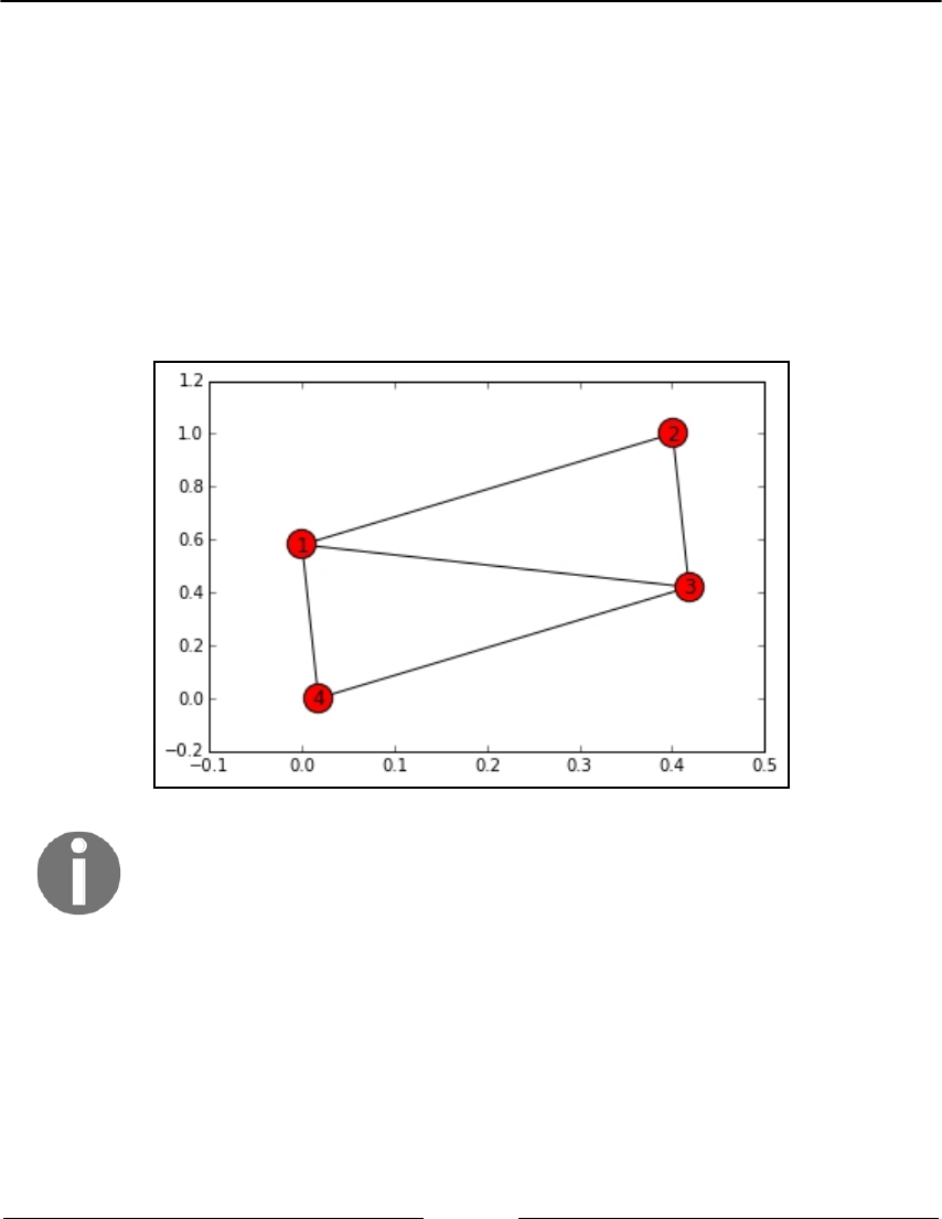
Social Network Analysis Chapter 6

[ 339 ]

An important measure of each node in a graph is their degree. In an undirected graph, the

degree of a node represents the number of links the node has. For directed graphs, there are

two types of degree: an in-degree and an out-degree. These count the inbound and

outbound links of the node, respectively.

Let's add a node (to unbalance the graph) and calculate the nodes' degrees, as follows:

In: G.add_edge(1, 3)

nx.draw_networkx(G)

plt.show()

The resulting plot of the graph is as follows:

The graphs in this chapter may be different to the ones obtained on your

local computer, because graphical layout initialization is made with

random parameters.

The degree of the nodes is displayed as follows:

In: G.degree()

Out: {1: 3, 2: 2, 3: 3, 4: 2}

Social Network Analysis Chapter 6

[ 340 ]

For large graphs, this measure is impractical since the output dictionary has an item for

every node. In such cases, a histogram of the nodes' degree is often used to approximate its

distribution. In the following example, a random network with 10,000 nodes and a link

probability of 1 % is built. Then, the histogram of the node degree is extracted, as follows:

In: k = nx.fast_gnp_random_graph(10000, 0.01).degree()

plt.hist(list(dict(k).values()))

The histogram for the preceding code is as follows:

Graph algorithms

To get insights from graphs, many algorithms have been developed. In this chapter, we'll

use a well-known graph in NetworkX, that is, the Krackhardt Kite graph. It is a dummy

graph containing 10 nodes, and it is typically used to proof graph algorithms. David

Krackhardt is the creator of the structure, which has the shape of a kite. It's composed of

two different zones. In the first zone (composed of nodes 0 to 6), the nodes are interlinked;

in the other zone (nodes 7 to 9), they are connected as a chain:

In: G = nx.krackhardt_kite_graph()

nx.draw_networkx(G)

plt.show()

Social Network Analysis Chapter 6

[ 341 ]

In the following plot, you can examine the Krackhardt Kite's graph structure:

Let's start with connectivity. Two nodes of a graph are connected if there is at least a path

(that is, a sequence of nodes) between them.

If at least one path exists, the shortest path between the two nodes is the one with the

shortest collection of nodes you should pass (or traverse) to go from the source to the

destination node.

Note that, in a directed graph, you must follow the link's directions.

In NetworkX, checking whether a path exists between two nodes, calculating the shortest

route, and getting its length is very easy. For example, to check the connectivity and the

path between nodes 1 and 9, you can use the following code:

In: print(nx.has_path(G, source=1, target=9))

print(nx.shortest_path(G, source=1, target=9))

print(nx.shortest_path_length(G, source=1, target=9))

Out: True

[1, 6, 7, 8, 9]

Social Network Analysis Chapter 6

[ 342 ]

This function just gives the shortest path from one node to another. What about if we want

to see all the paths to reach node 9 from node 1? An algorithm proposed by Jin Yen

provides this answer, and it's implemented in the function shortest_simple_paths in

NetworkX. This function returns a generator of all the paths, from the shortest to the

longest, between the node sources and the target in the graph:

In: print (list(nx.shortest_simple_paths(G, source=1, target=9)))

Out: [[1, 6, 7, 8, 9], [1, 0, 5, 7, 8, 9], [1, 6, 5, 7, 8, 9],

[1, 3, 5, 7, 8, 9], [1, 4, 6, 7, 8, 9], [1, 3, 6, 7, 8, 9],

[1, 0, 2, 5, 7, 8, 9], [...]]

Finally, another handy function provided by NetworkX is the

all_pairs_shortest_path function, which returns a Python dictionary containing the

shortest path between all of the pairs of nodes in the network. For example, to see the

shortest path from node 5, you just need to see what's inside key 5:

In: paths = list(nx.all_pairs_shortest_path(G))

paths[5][1]

Out: {0: [5, 0],

1: [5, 0, 1],

2: [5, 2],

3: [5, 3],

4: [5, 3, 4],

5: [5],

6: [5, 6],

7: [5, 7],

8: [5, 7, 8],

9: [5, 7, 8, 9]}

As expected, the paths between 5 and all the other nodes start with 5 itself. Note that this

structure is also a dictionary, and therefore, to obtain the shortest path between

nodes a and b, it can just be called paths[a][b]. Use this function carefully on large

networks. In fact, under the hood, it computes all the pairwise shortest paths with a

computational complexity of O(N

Social Network Analysis Chapter 6

[ 343 ]

Types of node centrality

We will now start talking about node centrality, which roughly represents the importance

of the node inside the network. It also gives an idea of how well the node connects the

network. There are multiple types of centrality that we will look at here, including

betweenness centrality, degree centrality, closeness centrality, harmonic centrality, and

eigenvector centrality.

Betweenness centrality: This type of centrality gives you an idea about the

number of shortest paths in which the node is present. Nodes with high

betweenness centrality are the core components of the network, and many

shortest paths route through them. In the following example, NetworkX offers a

straightforward way to compute the betweenness centrality of all the nodes:

In: nx.betweenness_centrality(G)

Out: {0: 0.023148148148148143,

1: 0.023148148148148143,

2: 0.0,

3: 0.10185185185185183,

4: 0.0,

5: 0.23148148148148148,

6: 0.23148148148148148,

7: 0.38888888888888884,

8: 0.2222222222222222,

9: 0.0}

As you can imagine, the highest betweenness centrality is achieved by node 7. It

seems very important since it's the only node that connects elements 8 and 9 (it's

their gateway to the network). On the contrary, nodes such as 9, 2, and 4 are on

the extreme border of the network, and they are not present in any of the shortest

paths of the network. Therefore, these nodes can be removed without affecting

the connectivity of the network.

Degree centrality: This type of centrality is simply the percentage of the vertexes

that are incident upon a node. Note that, in directed graphs, there are two degree

centralities for every node: that is in-degree and out-degree centrality. Let's take a

look at the following example:

In: nx.degree_centrality(G)

Out: {0: 0.4444444444444444,

1: 0.4444444444444444,

2: 0.3333333333333333,

3: 0.6666666666666666,

Social Network Analysis Chapter 6

[ 344 ]

4: 0.3333333333333333,

5: 0.5555555555555556,

6: 0.5555555555555556,

7: 0.3333333333333333,

8: 0.2222222222222222,

9: 0.1111111111111111}

As expected, node 3 has the highest degree centrality since it's the node with the

maximum number of links (it's connected to six other nodes). On the contrary,

node 9 is the node with the lowest degree since it has only one edge.

Closeness centrality: To compute this for every node, calculate the shortest path

distance to all other nodes, average it, divide the average by the maximum

distance, and take the inverse of that value. This results in a score between 0 (the

greater average distance) and 1 (the lower average distance). In our example, for

node 9, the shortest path distances are [1, 2, 3, 3, 4, 4, 4, 5, 5]. The average (3.44) is

then divided by 5 (the maximum distance) and subtracted from 1, resulting in a

closeness centrality score of 0.31. You can use the following code to compute the

closeness centrality for all the nodes in the example graph:

In: nx.closeness_centrality(G)

Out: {0: 0.5294117647058824,

1: 0.5294117647058824,

2: 0.5,

3: 0.6,

4: 0.5,

5: 0.6428571428571429,

6: 0.6428571428571429,

7: 0.6,

8: 0.42857142857142855,

9: 0.3103448275862069}

The nodes with high closeness centrality are 5, 6, and 3. In fact, they are the nodes

that are present in the middle of the network, and on average, they can reach all

the other nodes with a few hops. The lowest score belongs to node 9. In fact, its

average distance to reach all the other nodes is pretty high.

Social Network Analysis Chapter 6

[ 345 ]

Harmonic centrality: This measure is similar to closeness centrality, but instead

of having the inverse of the sum of the reciprocal of the distances, it has the sum

of reciprocal of distances. Doing so, it emphasizes the extremes of distances. Let's

see what the harmonic distances look like in our network:

In: nx.harmonic_centrality(G)

Out: {0: 6.083333333333333,

1: 6.083333333333333,

2: 5.583333333333333,

3: 7.083333333333333,

4: 5.583333333333333,

5: 6.833333333333333,

6: 6.833333333333333,

7: 6.0,

8: 4.666666666666666,

9: 3.4166666666666665}

Node 3 is the one with the highest harmonic centrality, while 5 and 6 have a

comparable but lower value. Again, those nodes are in the center of the network,

and on average, they can reach all the other nodes with a few hops. Opposite,

node 9 has the lowest harmonic centrality; in fact, it's the farthest from all the

other nodes on average.

Eigenvector centrality: If the graph is directed, the nodes represent web pages

and the edges represent page links. A slightly modified version is named

PageRank. This metric, invented by Larry Page, is the core ranking algorithm of

Google, as well as Bing, and possibly other search engines. It gives every node a

measure of how important the node is from the point of view of a random surfer.

Its name derives from the fact that if you think of the graph as a Markov Chain,

the graph represents the eigenvector associated with the greatest eigenvalue.

Therefore, from this point of view, this probabilistic measure represents the static

distribution of the probability of visiting a node. Let's take a look at the following

example:

In: nx.eigenvector_centrality(G)

Out: {0: 0.35220918419838565,

1: 0.35220918419838565,

2: 0.28583482369644964,

3: 0.481020669200118,

4: 0.28583482369644964,

5: 0.3976909028137205,

6: 0.3976909028137205,

7: 0.19586101425312444,

Social Network Analysis Chapter 6

[ 346 ]

8: 0.04807425308073236,

9: 0.011163556091491361}

In this example, nodes 3 and 9 have the highest and the lowest scores according

to the eigenvector centrality measure. Compared to degree centrality, eigenvalue

centrality gives an idea about the static distribution of the surfers across the

network because it considers, for each node, not only the directly connected

neighbors (as in degree centrality), but also the whole structure of the network. If

the graph represented web pages and their connections, this makes them the

most/least (probable) visited pages.

As a concluding topic, we'll introduce the clustering coefficient. In brief, it is the proportion

of the node's neighbors that are also neighbors with each other (that is, the proportion of

possible triplets or triangles that exist). Higher values indicate higher cliquishness. It's

named this way because it represents the degree to which nodes tend to cluster together.

Let's take a look at the following example:

In: nx.clustering(G)

Out: {0: 0.6666666666666666,

1: 0.6666666666666666,

2: 1.0,

3: 0.5333333333333333,

4: 1.0,

5: 0.5,

6: 0.5,

7: 0.3333333333333333,

8: 0.0,

9: 0.0}

Higher values can be seen in the highly connected sections of the graph and lower values

can be seen in the least connected areas.

Social Network Analysis Chapter 6

[ 347 ]

Partitioning a network

Now, let's look at the way in which you can partition the network into multiple

subnetworks of nodes. One of the most used algorithms is the Louvain method, which was

specifically created to accurately detect communities in large graphs (with a million nodes).

We will first introduce the modularity measure. This is a measure of the structure of the

graph (it's not node-oriented), whose formal math definition is very long and complex and

which is beyond the scope of this book (readers can find more information at

https://sites.google.com/site/findcommunities/). It intuitively measures the quality of

the division of a graph into communities, comparing the actual community linkage with a

random one. The modularity score falls between -0.5 and +1.0; the higher the value, the

better the division (there is a dense intragroup connectivity and a sparse intergroup

connectivity).

It's a two-step iterative algorithm: first, there's a local optimization, then a global one, then

a local again, and so on:

In the first step, the algorithm locally maximizes the modularity of small1.

communities.

Then, it aggregates the nodes of the same community and hierarchically builds a2.

graph whose nodes are the communities.

The method repeats these two steps iteratively until the maximum global3.

modularity score is reached.

To take a peek at this algorithm in a practical example, we first need to create a larger

graph. Let's consider a random network with 100 nodes:

In this example, we will build a graph with the powerlaw algorithm, which tries1.

to maintain an approximate average clustering.

For every new node added to the graph, an m number of random edges will also2.

be added to it, with each of them having a probability of p to create a triangle.

The source code is not included in NetworkX, but it's in a separate module3.

named community. An implementation of this algorithm is shown in the

following example:

In: import community

# Module for community detection and clustering

G = nx.powerlaw_cluster_graph(100, 1, .4, seed=101)

partition = community.best_partition(G)

for i in set(partition.values()):

print("Community", i)

Social Network Analysis Chapter 6

[ 348 ]

members = [nodes for nodes in partition.keys()

if partition[nodes] == i]

print(members)

values = [partition.get(node) for node in G.nodes()]

nx.draw(G, pos=nx.fruchterman_reingold_layout(G),

cmap = plt.get_cmap('jet'),

node_color = values,

node_size=150,

with_labels=False)

plt.show()

print ("Modularity score:", community.modularity(partition, G))

Out: Community 0

[0, 46, 50, 61, 73, 74, 75, 82, 86, 96]

Community 1

[1, 2, 9, 16, 20, 28, 29, 35, 57, 65, 78, 83, 89, 93]

[...]

Modularity score: 0.7941026425874911

The first output of the program is the list of communities detected in the graph (each

community is a collection of nodes). In this case, the algorithm detected eight groups. We

wanted to highlight that we didn't specify the number of output communities that we were

looking for, but it was automatically decided by the algorithm. That's a desirable feature

shared with not all the clustering algorithms (k-means, for example, needs the number of

clusters as a parameter).

Then, we printed the graph, assigning a different color to each community. You can see that

the colors are pretty homogeneous on the edge nodes:

Social Network Analysis Chapter 6

[ 349 ]

Lastly, the algorithm returns the modularity score of the solution: 0.79 (that's a pretty high

score).

The last algorithm that this short introduction about graphs is going to present is

coloring. It is a graphical way of assigning labels to the nodes, in a way that neighbors

(that is, nodes with a link) must have different labels (or colors). To explain why this

algorithm is important, we will use a practical example. Telecommunication networks are

composed of antennas at different frequencies spread across the Earth. Think about each

antenna as a node, and the frequency as a label of the node. If antennas are closer than a

defined distance—let's say close enough to cause interference—they're connected with an

edge. Can we find the lowest number of different frequencies to allocate (to minimize the

bill the company has to pay) and avoid interferences between close antennas (that is, by

allocating different frequencies to linked nodes)?

The solution is given by the graph-coloring algorithms. In theory, the solution of such a

class of algorithm is NP-hard, and it's almost impossible to find the optimal solution,

though there are many approximations to obtain suboptimal solutions quickly. NetworkX

implements a greedy approach to solve the coloring problem. What's returned by the

function is a dictionary containing, for each node (the key in the dictionary), the color (the

value of the key in the dictionary). As an example, let's see the allocation of colors in our

example graph, and then let's see it colored:

In: G = nx.krackhardt_kite_graph()

d = nx.coloring.greedy_color(G)

print(d)

nx.draw_networkx(G,

node_color=[d[n] for n in sorted(d.keys())])

plt.show()

Out:{3: 0, 5: 1, 6: 2, 0: 2, 1: 1, 2: 3, 4: 3, 7: 0, 8: 1, 9: 0}

Social Network Analysis Chapter 6

[ 350 ]

Here is the plot of the graph, using different colors for the linked nodes:

As expected, linked nodes have different colors. It seems that for this configuration of the

network, four colors were needed. If this were representing a telecommunications network,

it would show us that four frequencies were needed to avoid interference.

Graph loading, dumping, and sampling

Beyond NetworkX, graphs and networks can be generated and analyzed with other

software. One of the best open source multiplatform software that can be used for their

analysis is named Gephi. It's a visual tool and it doesn't require programming skills. It's

freely available at http://gephi.github.io.

As in machine learning datasets, even graphs have standard formats for storing, loading,

and exchanging. This way, you can create a graph with NetworkX, dump it to a file, and

then load and analyze it with Gephi.

One of the most frequently used formats is Graph Modeling Language (GML). Now, let's

see how we can dump a graph into a GML file:

In: dump_file_base = "dumped_graph"

# Be sure the dump_file file doesn't exist

def remove_file(filename):

import os

if os.path.exists(filename):

Social Network Analysis Chapter 6

[ 351 ]

os.remove(filename)

G = nx.krackhardt_kite_graph()

# GML format write and read

GML_file = dump_file_base + '.gml'

remove_file(GML_file)

to_string = lambda x: str(x)

nx.write_gml(G, GML_file, stringizer=to_string)

to_int = lambda x: int(x)

G2 = nx.read_gml(GML_file, destringizer = to_int)

assert(G.edges() == G2.edges())

In the preceding chunk of code, we did the following:

We removed the dumped file, if it did exist in the first place.1.

Then, we created a graph (the Kite), and after that, we dumped and loaded it.2.

Finally, we compared the original and the loaded structure, asserting that they're3.

equal.

Beyond GML, there are a variety of formats. Each of these formats has different features.

Note that some of them remove information pertaining to the network (like edge/node

attributes). Similar to the write_gml function and its equivalent, read_gml, are the

following ones (the names are self-explanatory):

The adjacency list (read_adjlist and write_adjlist)

The multiline adjacency list (read_multiline_adjlist and

write_multiline_adjlist)

The edge list (read_edgelist and write_edgelist)

GEXF (read_gexf and write_gexf)

Pickle (read_gpickle and write_gpickle)

GraphML (read_graphml and write_graphml)

LEDA (read_leda and parse_leda)

YAML (read_yaml and write_yaml)

Pajek (read_pajek and write_pajek)

GIS Shapefile (read_shp and write_shp)

JSON (load/loads and dump/dumps, and provides JSON serialization)

Social Network Analysis Chapter 6

[ 352 ]

The last topic of this chapter is sampling. Why sample a graph? We sample graphs because

working with large graphs is sometimes impractical (remember that in the best case, the

processing time is proportional to the graph size). Therefore, it's better to sample it, create

an algorithm by working on a small-scale scenario, and then test it on the full-scale

problem. There are several ways to sample a graph. Here, we're going to introduce the

three most frequently used techniques.

In the first technique, which is known as node sampling, a limited subset of nodes, along

with their links, forms the sampled set. In the second technique, which is known as link

sampling, a subset of links forms the sampled set. Both of these methods are simple and

fast, but they may potentially create a different structure for the network. The third method

is named snowball sampling. The initial node, all its neighbors, and the neighbors of the

neighbors (expanding the selection this way until we reach the maximum traversal depth

parameter) form the sampled set. In other words, the selection is like a rolling snowball.

Note that you can also subsample the traversed links. In other words, each

link has a probability of p that has to be followed and selected in the

output set.

The last sampling method is not a part of NetworkX, but you can find an implementation

for the same in the snowball_sampling.py file.

In this example, we will subsample the LiveJournal network by starting with the person

with an alberto ID and then expand recursively twice (in the first example) and three

times (in the second example). In the latter instance, every link is followed by a probability

of 20%, thus decreasing the retrieval time. Here is an example that demonstrates the same:

In: import snowball_sampling

import matplotlib.pyplot as plot

my_social_network = nx.Graph()

snowball_sampling.snowball_sampling(my_social_network, 2, 'alberto')

nx.draw(my_social_network)

ax = plot.gca()

ax.collections[0].set_edgecolor("#000000")

plt.show()

Out: Reching depth 0

new nodes to investigate: ['alberto']

Reching depth 1

new nodes to investigate: ['mischa', 'nightraven', 'seraph76',

'adriannevandal', 'hermes3x3', 'clymore', 'cookita', 'deifiedsoul',

'msliebling', 'ph8th', 'melisssa', '______eric_', 'its_kerrie_duhh',

'eldebate']

Social Network Analysis Chapter 6

[ 353 ]

Here is the result of the sampling code:

We will now proceed by using a specific sampling rate of 0.2:

In: my_sampled_social_network = nx.Graph()

snowball_sampling.snowball_sampling(my_sampled_social_network, 3,

'alberto', sampling_rate=0.2)

nx.draw(my_sampled_social_network)

ax = plot.gca()

ax.collections[0].set_edgecolor("#000000")

plt.show()

Out: Reching depth 0

new nodes to investigate: ['alberto']

Reching depth 1

new nodes to investigate: ['mischa', 'nightraven', 'seraph76',

'adriannevandal', 'hermes3x3', 'clymore', 'cookita', 'deifiedsoul',

'msliebling', 'ph8th', 'melisssa', '______eric_', 'its_kerrie_duhh',

'eldebate']

Reching depth 2

new nodes to investigate: ['themouse', 'brynna', 'dizzydez', 'lutin',

'ropo', 'nuyoricanwiz', 'sophia_helix', 'lizlet', 'qowf', 'cazling',

'copygirl', 'cofax7', 'tarysande', 'pene', 'ptpatricia', 'dapohead',

'infinitemonkeys', 'noelleleithe', 'paulisper', 'kirasha',

'lenadances',

'corianderstem', 'loveanddarkness', ...]

Social Network Analysis Chapter 6

[ 354 ]

The resulting graph is more detailed:

Summary

In this chapter, we learned what a social network is, including its creation and

modification, representation, and some of the important measures of the social network

and its nodes. Finally, we discussed the loading and saving of large graphs and ways to

deal with the same.

With this chapter, almost all of the essential data science algorithms have been presented.

Machine learning techniques were discussed in Chapter 4, Machine Learning, and social

network analysis methods were discussed here. We will finally discuss the most advanced

and cutting-edge techniques of deep learning and neural networks in the next chapter, Deep

Learning Beyond the Basics.

Deep Learning Beyond the

Basics

In this chapter, we will introduce deep models, and we will show three examples of how to

build deep models. More specifically, in this chapter, you'll learn the following:

The basics of deep learning

How to optimize a deep net

The speed/complexity/accuracy problem

How to classify images with a CNN

How to use a pre-trained network for classification and transfer learning

How to operate on sequences using a LSTM

We will be using the Keras package (https:/󰜌/󰜌keras.󰜌io/󰜌), which is a high-level API for

deep learning that will render approaching neural networks for deep learning much easier

and more understandable because it is characterized by a Lego-like approach (here, the

bricks are a neural network's composing elements).

Approaching deep learning

Deep learning is an extension of the classical machine-learning approach using neural

networks: instead of building networks of a few layers (so-called shallow networks), we can

stack hundreds of layers to create an elaborate, but more powerful, learner. Deep learning

is one of the most popular methods of artificial intelligence (AI) nowadays since it's very

effective and helps to solve many problems in pattern recognition, such as object or

sequence identification, which seemed unbreakable using standard machine learning tools.

Deep Learning Beyond the Basics Chapter 7

[ 356 ]

The idea of neural networks came from the human central nervous system, where multiple

nodes (or neurons) that are able to process simple information are connected together to

create a network capable of processing complex information. In fact, neural networks are

so named because they can learn the weights of the model autonomously and adaptively,

and, given enough complex network architecture, they're able to approximate any

nonlinear function. In deep learning, the nodes are usually called units or neurons.

Let's see how a deep architecture is built and what its components are. We will start with a

small deep architecture for a classification problem composed of three layers, as shown in

the following figure:

This network has the following characteristics:

It has three layers. The left-hand one is called the input layer, the right-hand one

is called the output layer, and the central one is the hidden layer. Generically, in

a neural network, there is always one input and one output layer, and zero or

more hidden layers (when there are zero hidden layers, the whole neural

architecture will effectively turn into a logistic-regression system).

The input layer is composed of five units, which means that each observation

vector is composed of five numerical features (that is, the observation matrix has

five columns). Note that the features must be numeric and in a bounded range of

values (for better numeric convergence, the range is ideally 0 to +1, but -1 to +1 is

also fine). Therefore, categorical features must be preprocessed in order to

become numerical.

Deep Learning Beyond the Basics Chapter 7

[ 357 ]

The output layer is composed of three units, which means we want to

differentiate among three output classes (that is, perform a three-class

classification). In the case of a regression problem, there should be just one unit

in this layer.

The hidden layer is composed of eight units. Note that there's no rule about how

many hidden layers should appear in the deep architecture and how many units

each should have. These parameters are left to the scientist, and, usually, they

require some optimization and fine-tuning in order to work best.

Each connection has a weight associated with it. This is optimized during the

learning algorithm.

Each unit of the input layer is connected to all the units of the next layer.

There are neither connections between the units in the same layers nor

connections between units in two of the layers at a distance greater than 1

from each other.

In the example, the flow of information is passed forward, from the input to the output

(passing eventually through the hidden layers); in literature, this network is referred to as a

feed-forward neural network.

How does it create the final prediction? Let's see how it works step by step:

Starting from the top unit of the hidden layer, it performs a dot product between1.

the output vector of the first layer (that is, the input-observation vector) and the

vector of weights of the connections between the first layer and the first unit of

the hidden layer.

The value is then transformed with the activation function of the unit.2.

This operation is repeated for all the units in the hidden layer.3.

Finally, we can compute the feed-forward propagated values between the hidden4.

layer and the output layer in the same way, which produces the outputs of the

network.

The process seems very easy, and it's composed of multiple embarrassingly parallel tasks.

The last missing point of the explanation is the activation function: What is it and why is it

needed? The activation function helps to make binary decisions more separable (it makes

the decision boundary non-linear, thus helping to separate the examples better) and it's a

property (or an attribute) of each unit; ideally, each unit should have a different activation

function, although they're usually grouped by layer.

Deep Learning Beyond the Basics Chapter 7

[ 358 ]

Typical activation functions are the sigmoid, the hyperbolic tangent, and the softmax (for

classification problems) functions, although one of the most popular currently is the

rectified linear unit (or ReLU), whose output is the maximum between 0 and the input

(where the input is the dot product between the previous layer output and the weights of

the connections).

The activation function, as the number of units and the number of hidden layers, is a

parameter of a deep network and should be optimized by the scientist to obtain a better

performance.

Training a neural network characterized by many layers is a hard operation since there is a

very high number (sometimes millions) of parameters to tune: the weights. The most

common way to assign weights to connections uses a similar approach to a gradient

descent, and it's called backpropagation, because it propagates back the errors from the

output layer toward the input layer, updating each weight proportionally to the gradient of

the error at that point in the network. Initially, weights are assigned at random, but, after a

few steps, they should converge toward the optimal value.

This was a very short introduction to deep learning and neural networks; if you find the

topic interesting and you want to dig more into it, we recommend the following video

series from Packt, where you can find a better explanation and some nice tricks to master

the learning process:

Deep Learning with Python [Video] (https:/󰜌/󰜌www.󰜌packtpub.󰜌com/󰜌big-󰜌data-󰜌and-

business-󰜌intelligence/󰜌deep-󰜌learning-󰜌python-󰜌video)

Deep Learning with TensorFlow [Video] (https:/󰜌/󰜌www.󰜌packtpub.󰜌com/󰜌big-󰜌data-

and-󰜌business-󰜌intelligence/󰜌deep-󰜌learning-󰜌tensorflow-󰜌video)

Now let's see something practical: how to solve a classification problem with neural

networks. We will use Keras in this example. The first is a Python library for low-level

primitives, which is typically used in deep learning and is able to take advantage of recent

GPUs and numerical speed-up to process multi-dimensional arrays efficiently. Keras is an

advanced, fast, and modular Python library for neural networks able to run on top of

different numerical computation frameworks, such as TensorFlow, Microsoft Cognitive

Tool (previously named CNTK), or Theano.

Deep Learning Beyond the Basics Chapter 7

[ 359 ]

Classifying images with CNN

Let's now apply a deep neural network to an image-classification problem. Here, we will

try to predict a traffic sign from its image. For this task, we will use a CNN (convolutional

neural network), which is able to exploit the spatial correlation between nearby pixels in an

image, and is the state of the art in deep learning when working on this kind of problem.

The dataset is available here: http:/󰜌/󰜌benchmark.󰜌ini.󰜌rub.󰜌de/󰜌?󰜌section=

gtsrb󰜌subsection=󰜌dataset. We would like to thank the team for having

released the dataset free of charge, and reference the publication dealing

with this dataset:

J. Stallkamp, M. Schlipsing, J. Salmen, and C. Igel. The German Traffic Sign

Recognition Benchmark: A multi-class classification competition. In Proceedings

of the IEEE International Joint Conference on Neural Networks, pages

1453–1460. 2011.

First, download the dataset and then unzip it. The filename of the dataset

is GTSRB_Final_Training_Images.zip, and, when unzipped, you'll find a new directory

named GTSRB, which contains all the images located in the same directory as the Jupyter

notebook.

The next step is to import Keras and check if the backend is configured properly. In this

chapter, we will use the TensorFlow backend, and all the code is tested on that backend.

The backend choice is reversible. If you want to switch from TensorFlow

to another backend, follow the guide here: https:/󰜌/󰜌keras.󰜌io/󰜌backend.

Scripts that are written using Keras can operate successfully no matter

what backend they use (the performance in terms of computation time

and minimized errors may differ, though).

To check your backend, run the following code, and check if the operation performs

successfully and the resulting output matches that reported here.

In: import keras

Out: Using TensorFlow backend.

It's now time to start the processing, so we have to define some static parameters for the

task. There are two of these, primarily: the number of different signals we want to

recognize (that is, the number of classes) and the size of the pictures. The number of classes

is 43; that is, we have 43 different traffic signs to recognize.

Deep Learning Beyond the Basics Chapter 7

[ 360 ]

The second parameter, the image size, is important because the input images can be of

different sizes and shapes; we need to resize them to a standard size in order to run our

deep net on them. We picked 32x32 pixels as the standard: it's small enough to recognize

the signal, and, at the same time, it doesn't require too much memory (that is, every

grayscale image uses just 1,024 bytes or 1 KB). Increasing the size means increasing the

memory needed to keep the dataset, plus the input layer of the deep net and the time

necessary for computations. In the literature, 32x32 is a pretty standard choice for images

with just one item; so, in our case, we have good reasons to decide on that size.

In: N_CLASSES = 43

RESIZED_IMAGE = (32, 32)

At this point, we have to read the images and resize them, creating the observation matrix

and the array of labels. To do so, we perform the following steps:

Import the modules needed for the processing. The most important is Scikit-1.

learn, or sklearn, which contains loads of functions to process the images.

We read the images one after another. The label is contained in the path. For2.

example, the image

GTSRB/Final_Training/Images/00000/00003_00024.ppm has label 00000,

which is

; and the

image GTSRB/Final_Training/Images/00025/00038_00005.ppm has label

00025, which is 25. The label is stored as a labeled-encoded array, which is an

array 43-cells long with only one that has a value of 1 (all the others are

The image is stored in the PPM (Portable PixMap) format, and it's a lossless way3.

to store the pixels in an image. Scikit-image, or just skimage (https:/󰜌/󰜌scikit-

image.󰜌org/󰜌), is able to read that format by using the function imread. If you

don't have Scikit-image already installed on your system, just type the following

in a shell: conda install scikit-image or pip install -U scikit-

image. The returned object is a 3D NumPy array.

The 3D NumPy array, containing the pixel representation of the image (with4.

three channels—red, blue and green) is then converted to grayscale. Here, we

first convert to the LAB color space (see https:/󰜌/󰜌hidefcolor.󰜌com/󰜌blog/󰜌color-

management/󰜌what-󰜌is-󰜌lab-󰜌color-󰜌space—this color space is more perceptually

linear than others, which implies that the same amount of change in a color value

should produce an impact of the same visual importance), and then the first

channel (containing the luminance) is kept. Again, this operation is easily done

with skimage. As a result, we have a 1D NumPy array containing the image

pixels.

The image is finally resized to the 32x32 pixel format, again using5.

a skimage function.

Deep Learning Beyond the Basics Chapter 7

[ 361 ]

Finally, all the images are squeezed into a 4-dimensional matrix: the first6.

dimension is used to index the image within the dataset; the second and the third

represent the height and the width of the image, respectively; and the last

dimension is the channel. Having 39,208 images, with all 32x32 pixels in

grayscale, the observation matrix is therefore in the shape (39,208, 32, 32, 1).

Labels are compacted into a two-dimensional matrix. The first dimension is the7.

index of the image and the second dimension is the class. Due to having the same

number of images, and 43 possible classes, this matrix will be shaped (39,208,

43).

The following shows all seven steps translated into code:

In: import matplotlib.pyplot as plt

import glob

from skimage.color import rgb2lab

from skimage.transform import resize

from collections import namedtuple

import numpy as np

np.random.seed(101)

%matplotlib inline

Dataset = namedtuple('Dataset', ['X', 'y'])

def to_tf_format(imgs):

return np.stack([img[:, :, np.newaxis] for img in imgs],

axis=0).astype(np.float32)

def read_dataset_ppm(rootpath, n_labels, resize_to):

images = []

labels = []

for c in range(n_labels):

full_path = rootpath + '/' + format(c, '05d') + '/'

for img_name in glob.glob(full_path + "*.ppm"):

img = plt.imread(img_name).astype(np.float32)

img = rgb2lab(img / 255.0)[:,:,0]

if resize_to:

img = resize(img, resize_to, mode='reflect',

anti_aliasing=True)

label = np.zeros((n_labels, ), dtype=np.float32)

label[c] = 1.0

images.append(img.astype(np.float32))

labels.append(label)

return Dataset(X = to_tf_format(images).astype(np.float32),

y = np.matrix(labels).astype(np.float32))

dataset = read_dataset_ppm('GTSRB/Final_Training/Images', N_CLASSES,

Deep Learning Beyond the Basics Chapter 7

[ 362 ]

RESIZED_IMAGE)

print(dataset.X.shape)

print(dataset.y.shape)

Out: (39209, 32, 32, 1)

(39209, 43)

The dataset is composed of almost 40,000 images; let's see what the first of them looks like,

after the color change and the resize:

In: plt.imshow(dataset.X[0, :, :, :].reshape(RESIZED_IMAGE))

print("Label:", dataset.y[0, :])

Out: Label: [[1. 0. 0. 0. 0. 0. 0. 0. 0. 0. 0. 0. 0. 0. 0. 0. 0. 0. 0. 0.

0. 0. 0. 0. 0. 0. 0. 0. 0. 0. 0. 0. 0. 0. 0. 0. 0. 0. 0. 0.

0. 0. 0.]]

The following is the plotted sample image:

Even though the image has a very low definition, 32x32 pixels, we can immediately

recognize which sign is represented. So far, it seems that the reshaping operation is leaving

the images intelligible, even to humans. Note again that the label is a 43-dimensional

vector; since this image belongs to the first class (that is, class 00000), just the first element

of the label is not null.

Deep Learning Beyond the Basics Chapter 7

[ 363 ]

Another element, of a different class, is shown as follows. That's image number 1,000 in the

dataset, and its class is the 2

(in fact, it's a different sign):

Let's now split the dataset into training and testing. We use Scikit-learn to randomly

separate and shuffle the images. In this cell, we select 25% of the dataset as a test set; that is,

almost 10,000 images, leaving the other 29K+ images for training the deep net:

In: from sklearn.model_selection import train_test_split

idx_train, idx_test = train_test_split(range(dataset.X.shape[0]),

test_size=0.25,

random_state=101)

X_train = dataset.X[idx_train, :, :, :]

X_test = dataset.X[idx_test, :, :, :]

y_train = dataset.y[idx_train, :]

y_test = dataset.y[idx_test, :]

print(X_train.shape)

print(y_train.shape)

print(X_test.shape)

print(y_test.shape)

Out: (29406, 32, 32, 1)

(29406, 43)

(9803, 32, 32, 1)

(9803, 43)

Deep Learning Beyond the Basics Chapter 7

[ 364 ]

Here's the moment of creating a convolutional deep network. We start with a simple, easy

to understand, neural network. Then we'll move to something that is more complex but

accurate.

Creating deep nets with Keras is very easy: you have to define all layers in a sequential

way, one after another. The Keras object needs to define the layers in a sequence named

Sequential. Here, we will create a deep net with three layers:

The input layer, defined as a convolutional 2D layer (which is actually a1.

convolutional operation between the image and the kernel), contains 32 filters in

the shape of 3x3 pixels and with an activation layer of type ReLU.

A layer that flattens the output of the previous; that is, square observations will2.

be unrolled to create a 1D array.

A dense output layer, with softmax activation and which is composed of 433.

units, one for each class.

The model is then compiled and, finally, fitted to the training data. During this operation

we selected the following:

The optimizer: SGD, the simplest one

The batch size: 32 images/batch

The numbers of epochs: 10

Here is the code that will generate the model we have just described:

In: from keras.models import Sequential

from keras.layers.core import Dense, Flatten

from keras.layers.convolutional import Conv2D

from keras.optimizers import SGD

from keras import backend as K

K.set_image_data_format('channels_last')

def cnn_model_1():

model = Sequential()

model.add(Conv2D(32, (3, 3),

padding='same',

input_shape=(RESIZED_IMAGE[0], RESIZED_IMAGE[1], 1),

activation='relu'))

model.add(Flatten())

model.add(Dense(N_CLASSES, activation='softmax'))

return model

cnn = cnn_model_1()

Deep Learning Beyond the Basics Chapter 7

[ 365 ]

cnn.compile(loss='categorical_crossentropy',

optimizer=SGD(lr=0.001, decay=1e-6),

metrics=['accuracy'])

cnn.fit(X_train, y_train,

batch_size=32,

epochs=10,

validation_data=(X_test, y_test))

Out: Train on 29406 samples, validate on 9803 samples

Epoch 1/10

29406/29406 [==============================] - 11s 368us/step -

loss: 2.7496 - acc: 0.5947 - val_loss: 0.6643 - val_acc: 0.8533

Epoch 2/10

29406/29406 [==============================] - 10s 343us/step -

loss: 0.4838 - acc: 0.8937 - val_loss: 0.4456 - val_acc: 0.9001

[...]

Epoch 9/10

29406/29406 [==============================] - 10s 337us/step -

loss: 0.0739 - acc: 0.9876 - val_loss: 0.2306 - val_acc: 0.9553

Epoch 10/10

29406/29406 [==============================] - 10s 343us/step -

loss: 0.0617 - acc: 0.9897 - val_loss: 0.2208 - val_acc: 0.9574

The final accuracy is close to 99% on the training set and almost 96% on the test set. We're

overfitting a bit, but let's see the confusion matrix and the classification report of this model

on the test set. We'll also print the log2 of the confusion matrix to better identify

misclassifications.

To do so, we first need to predict the labels and then apply the argmax operator to select

the most likely class:

In: from sklearn.metrics import classification_report, confusion_matrix

def test_and_plot(model, X, y):

y_pred = cnn.predict(X)

y_pred_softmax = np.argmax(y_pred, axis=1).astype(np.int32)

y_test_softmax = np.argmax(y, axis=1).astype(np.int32).A1

print(classification_report(y_test_softmax, y_pred_softmax))

cm = confusion_matrix(y_test_softmax, y_pred_softmax)

plt.imshow(cm, interpolation='nearest', cmap=plt.cm.Blues)

plt.colorbar()

plt.tight_layout()

plt.show()

# And the log2 version, to emphasize the misclassifications

plt.imshow(np.log2(cm + 1), interpolation='nearest',

cmap=plt.get_cmap("tab20"))

plt.colorbar()

Deep Learning Beyond the Basics Chapter 7

[ 366 ]

plt.tight_layout()

plt.show()

test_and_plot(cnn, X_test, y_test)

Out:

precision recall f1-score support

0 0.87 0.90 0.88 67

1 0.97 0.94 0.95 539

2 0.93 0.94 0.94 558

[........]

40 0.93 0.96 0.95 85

41 0.92 0.94 0.93 47

42 1.00 0.91 0.95 53

avg / total 0.96 0.96 0.96 9803

The following are the diagnostic plots, which provide you with evidence on the

performance of the model:

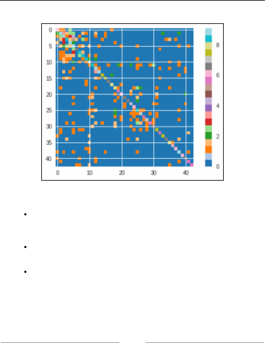
Deep Learning Beyond the Basics Chapter 7

[ 367 ]

And here's the log2 version of the confusion matrix:

The classification already seems to be pretty good. Can we do something better and avoid

the overfitting? Yes, here is what we can use:

Dropout layers: This is the equivalent of regularization, and it prevents

overfitting. Basically, at each step during the training, a portion of units is

deactivated, so the output of the layer doesn't rely too much on just a few of

them.

BatchNormalization layer: This z-normalizes the layer, by subtracting the batch

mean and dividing it by the standard deviation. It's useful for recentering the

data, and it amplifies/attenuates the signal at each step.

MaxPooling: This is a nonlinear transformation, which is used to downsample

the input by applying a max filter to each region under the kernel. It's used to

select the max feature, which can be in a slightly different position within the

same class.

Deep Learning Beyond the Basics Chapter 7

[ 368 ]

Beyond these, there's always space to change the deep net and training properties; that is,

the optimizer (and its parameters), the batch size, and the number of epochs. Here, in the

next cell, is an improved deep net with the following layers:

Convolutional layer, with 32 3x3 filters and ReLU activation1.

BatchNormalization layer2.

Another convolutional layer followed by a BatchNormalization layer3.

Dropout layer, with a probability of 0.4 of being dropped4.

Flattening layer5.

512-units dense layer, with ReLU activation6.

BatchNormalization layer7.

Dropout layer, with a probability of 0.5 of being dropped8.

Output layer; as in the previous example, this is a softmax dense layer with 439.

units

How will that perform on our dataset?

In: from keras.layers.core import Dropout

from keras.layers.pooling import MaxPooling2D

from keras.optimizers import Adam

from keras.layers import BatchNormalization

def cnn_model_2():

model = Sequential()

model.add(Conv2D(32, (3, 3), padding='same',

input_shape=(RESIZED_IMAGE[0], RESIZED_IMAGE[1], 1),

activation='relu'))

model.add(BatchNormalization())

model.add(Conv2D(32, (3, 3),

padding='same',

input_shape=(RESIZED_IMAGE[0], RESIZED_IMAGE[1], 1),

activation='relu'))

model.add(BatchNormalization())

model.add(MaxPooling2D(pool_size=(2, 2)))

model.add(Dropout(0.4))

model.add(Flatten())

model.add(Dense(512, activation='relu'))

model.add(BatchNormalization())

model.add(Dropout(0.5))

model.add(Dense(N_CLASSES, activation='softmax'))

return model

cnn = cnn_model_2()

cnn.compile(loss='categorical_crossentropy',

Deep Learning Beyond the Basics Chapter 7

[ 369 ]

optimizer=Adam(lr=0.001, decay=1e-6), metrics=['accuracy'])

cnn.fit(X_train, y_train,

batch_size=32,

epochs=10,

validation_data=(X_test, y_test))

Out: Train on 29406 samples, validate on 9803 samples

Epoch 1/10

29406/29406 [==============================] - 24s 832us/step -

loss: 0.7069 - acc: 0.8145 - val_loss: 0.1611 - val_acc: 0.9584

Epoch 2/10

29406/29406 [==============================] - 23s 771us/step -

loss: 0.1784 - acc: 0.9484 - val_loss: 0.1065 - val_acc: 0.9714

[...]

Epoch 10/10

29406/29406 [==============================] - 23s 770us/step -

loss: 0.0370 - acc: 0.9878 - val_loss: 0.0332 - val_acc: 0.9920

<keras.callbacks.History at 0x7fd7ac0f17b8>

The training set's accuracy is similar to that for the test set, and they're both around 99%;

that is, 99 out of 100 images are classified with the correct label! This network is longer and

it requires more memory and computational power, but it's less prone to overfitting and it

performs better.

Let's now see the classification report and the confusion matrix (the full one and the log2

version):

In: test_and_plot(cnn, X_test, y_test)

Out:

precision recall f1-score support

0 1.00 0.97 0.98 67

1 1.00 0.98 0.99 539

2 0.99 1.00 0.99 558

[..........]

38 1.00 1.00 1.00 540

39 1.00 1.00 1.00 60

40 1.00 1.00 1.00 85

41 0.98 0.96 0.97 47

42 1.00 1.00 1.00 53

avg / total 0.99 0.99 0.99 9803

Deep Learning Beyond the Basics Chapter 7

[ 370 ]

Here are the visual representations of the results:

It is clear that the number of misclassifications has decreased quite significantly. Now, let's

try to do something better, by changing the parameters.

Deep Learning Beyond the Basics Chapter 7

[ 371 ]

Using pre-trained models

As you saw in the previous example, increasing the complexity of the network increases the

time and the memory needed to train it. Sometimes, we have to accept that we don't have a

machine powerful enough to try all the combinations. What can we do in that situation?

Basically, we can do two things:

Simplify the network; that is, by removing parameters and variables

Use a pre-trained network, which has already been trained by someone with a

powerful enough machine

In both situations, we will work in sub-optimal conditions, since the deep network won't be

as powerful as the one we could have used. More specifically, in the first case, the network

won't be very accurate because we have fewer parameters; in the second case, well, we

have to cope with someone else's decisions and training set. Although it's not very easy to

do, pre-trained models can also be fine-tuned with your dataset; in this case, the network

won't have a random initialization of the parameters. Although this is very interesting, this

operation is out of the scope of this book.

In this section, we will quickly show how to use pre-trained models, which is a common

way to proceed. Bear in mind that pre-trained models can be used in multiple situations:

Feature augmentation, to add a feature (in this case, the predicted label), along

with observation vectors, into your model

Transfer learning, to add more features (coefficients coming from one or model

layers), along with observation vectors, into your model

Prediction; that is, to compute the label

Let's now see how to use a pre-trained network to serve our purpose.

In Keras, various pre-trained models are available from

here: https://keras.io/applications.

Let's first download some images to test. In the following example, we will use the dataset

provided by Caltech, which is available here: http:/󰜌/󰜌www.󰜌vision.󰜌caltech.󰜌edu/󰜌Image_

Datasets/󰜌Caltech101/󰜌.

We would like to thank the authors of the dataset, and suggest to read

their paper: L. Fei-Fei, R. Fergus and P. Perona. One-Shot learning of object

categories. IEEE Trans. Pattern Recognition and Machine Intelligence.

Deep Learning Beyond the Basics Chapter 7

[ 372 ]

It contains several images in 101 categories and comes in the tar.gz format.

Now, with a new notebook, import the modules we will use. In this example, we will use

the InceptionV3 pre-trained network, which is able to recognize objects in images very well.

It has been developed by Google, and its output is comparable to the human eye.

First, we import the functions that are needed to set up the network, to1.

preprocess the inputs, and to extract the predictions:

In: from keras.applications.inception_v3 import InceptionV3

from keras.applications.inception_v3 import preprocess_input

from keras.applications.inception_v3 import decode_predictions

from keras.preprocessing import image

import numpy as np

import matplotlib.pyplot as plt

%matplotlib inline

Out: Using TensorFlow backend.

Now, let's load the huge network and its coefficient:2.

In: model = InceptionV3(weights='imagenet')

It's simple, isn't it?

The next step (and the final one) is to create a function to make the prediction. In3.

this case, we will predict the top three labels:

In: def predict_top_3(model, img_path):

img = image.load_img(img_path, target_size=(299, 299))

plt.imshow(img)

x = image.img_to_array(img)

x = np.expand_dims(x, axis=0)

x = preprocess_input(x)

preds = model.predict(x)

print('Predicted:', decode_predictions(preds, top=3)[0])

Deep Learning Beyond the Basics Chapter 7

[ 373 ]

Basically, this function loads and resizes the image to 299x299 pixels (which is the

default input size for the pre-trained network InceptionV3), and converts the image to the

correct format for the model. After that, it predicts all the labels of the image and selects

(and prints) the top three.

Let's see how it performs with an example image by using the pre-trained model and

asking for the top three predictions in terms of probability:

In: predict_top_3(model, "101_ObjectCategories/umbrella/image_0001.jpg")

The image we want to predict and the resulting output from the top three predictions are as

follows:

Out: Predicted: [('n04507155', 'umbrella', 0.88384396),

('n04254680', 'soccer_ball', 0.07257448),

('n03888257', 'parachute', 0.012849103)]

We confirm that this is a great result; the first label (with a score of 88%) is an umbrella,

followed by a soccer ball and a parachute. Let's now test a certainly more difficult image,

which is one whose label is not included in the InceptionV3 training set:

In: predict_top_3(model, "101_ObjectCategories/bonsai/image_0001.jpg")

Deep Learning Beyond the Basics Chapter 7

[ 374 ]

Here is the image and its top three results:

Out: Predicted: [('n02704792', 'amphibian', 0.20315942),

('n04389033', 'tank', 0.07383019),

('n04252077', 'snowmobile', 0.055828683)]

As expected, as it is not among its pre-defined classes, the network is not able to recognize

the bonsai in the first predicted label.

Actually, pre-trained models can be taught to recognize even completely

new classes by the so-called transfer learning technique. This technique is

out of the scope of this book, but you can read about it on this example

from Keras's blog: https:/󰜌/󰜌blog.󰜌keras.󰜌io/󰜌building-󰜌powerful-󰜌image-

classification-󰜌models-󰜌using-󰜌very-󰜌little-󰜌data.󰜌html.

Finally, let's see how to extract features from the intermediate layers, as follows:

As the first step, let's verify the label names:1.

In: print([l.name for l in model.layers])

Out: ['input_1', 'conv2d_1', 'batch_normalization_1',

..........

'activation_94', 'mixed10', 'avg_pool', 'predictions']

Deep Learning Beyond the Basics Chapter 7

[ 375 ]

We can select any of these layers; we will go for the one before the softmax2.

prediction. Let's create an object Model whose output is the avg_pool layer:

In: from keras.models import Model

feat_model = Model(inputs=model.input,

outputs=model.get_layer('avg_pool').output)

def extract_features(feat_model, img_path):

img = image.load_img(img_path, target_size=(299, 299))

x = image.img_to_array(img)

x = np.expand_dims(x, axis=0)

x = preprocess_input(x)

return feat_model.predict(x)

Finally, to extract the features for a picture, let's call the previous function with3.

an image:

In: f = extract_features(feat_model,

"101_ObjectCategories/bonsai/image_0001.jpg")

print(f.shape)

print(f)

Out: (1, 2048)

[[0.12340261 0.0833823 0.7935947 ... 0.50869745 0.34015656]]

As you can check, the avg_pool layer contains 2048 units, and the output of the function is

exactly a 2,048D array. You can now concatenate this array to any other feature array of

your choice.

Working with temporal sequences

The last example in this chapter is about dealing with temporal sequences; more

specifically, we will see how to deal with text, which is a variable-length sequence of

words.

Some data-science algorithms deal with text using the bag-of-words approach; that is, they

don't care where the words are and how they're placed in the text, they just care about their

presence/absence (and maybe their frequency). Instead, a special class of deep networks is

specifically designed to operate on sequences, where the order is important.

Deep Learning Beyond the Basics Chapter 7

[ 376 ]

Some examples are as follows:

Predict a future stock price, given its historical data: In this case, the input is a

sequence of numbers, and the output is a number

Predict whether the market will go up or down: In this case, given a sequence of

numbers, we want to predict a class (up or down)

Translate an English text to French: In this case, the input sequence is converted

into another sequence

Chatbot: In this case, the input and the output are both sequences (in the same

language)

For this example, let's do something easy. We will try to detect the sentiment of a movie

review. In this specific example, the input data is a sequence of words (and the order

counts!), and the output is a binary label (which is the sentiment positive or negative).

Let's start importing the dataset. Fortunately, Keras already includes this dataset, and it's

already pre-indexed; that is, each review is not composed of words but of indexes of a

dictionary. Also, it's possible to select just the top words, and, with this code, we select a

dictionary containing the top 25000 words:

In: from keras.datasets import imdb

((data_train, y_train),

(data_test, y_test)) = imdb.load_data(num_words=25000)

Let's see what's inside the data and the shape:

In: print(data_train.shape)

print(data_train[0])

print(len(data_train[0]))

Out: (25000,)

[1, 14, 22, 16, 43, 530, .......... 19, 178, 32]

218

Firstly, there are 25000 reviews; that is, observations. Secondly, each review is composed of

a sequence of numbers between 1 and 24,999; 1 indicates the start of the sequence, while the

last number signals a word that is not in the dictionary. Note that each review has a

different size; for example, the first one is 218 words in length.

Deep Learning Beyond the Basics Chapter 7

[ 377 ]

It's now time to trim or pad all the sequences to a specific size. With Keras, this is easily

done, and, for padding, the integer

is added:

In: from keras.preprocessing.sequence import pad_sequences

X_train = pad_sequences(data_train, maxlen=100)

X_test = pad_sequences(data_test, maxlen=100)

Our training matrix now has a rectangular shape. The first element after the

trimming/padding operation becomes the following:

In: print(X_train[0])

print(X_train[0].shape)

Out: [1415, .......... 19, 178, 32]

(100,)

For this observation, just the last 100 words are maintained. Overall, now, all the

observations have 100 dimensions. Let's now create a temporal deep model to predict the

review sentiment.

The model proposed here has three layers:

An embedding layer. The original dictionary is set to 25,000 words, and the1.

number of units composing the embedding (that is, the layer's output) is 256.

An LSTM layer. LSTM stands for long short-term memory, and it's one of the2.

most powerful deep models for sequences. Thanks to its deep architecture, it's

able to extract information from close and distant words in the sequence (hence

the name). In this example, the number of cells is set to 256 (as the previous layer

output dimension), with a dropout of 0.4 for regularization.

A dense layer with a sigmoid activation. That's what we need for a binary3.

classifier.

Here's the code for doing so:

In: from keras.models import Sequential

from keras.layers import LSTM, Dense

from keras.layers.embeddings import Embedding

from keras.optimizers import Adam

model = Sequential()

model.add(Embedding(25000, 256, input_length=100))

model.add(LSTM(256, dropout=0.4, recurrent_dropout=0.4))

model.add(Dense(1, activation='sigmoid'))

model.compile(loss='binary_crossentropy',

optimizer=Adam(),

metrics=['accuracy'])

Deep Learning Beyond the Basics Chapter 7

[ 378 ]

model.fit(X_train, y_train,

batch_size=64,

epochs=10,

validation_data=(X_test, y_test))

Out: Train on 25000 samples, validate on 25000 samples

Epoch 1/10

25000/25000 [==============================] - 139s 6ms/step -

loss:0.4923 - acc:0.7632 - val_loss:0.4246 - val_acc:0.8144

Epoch 2/10

25000/25000 [==============================] - 139s 6ms/step -

loss:0.3531 - acc:0.8525 - val_loss:0.4104 - val_acc: 0.8235

Epoch 3/10

25000/25000 [==============================] - 138s 6ms/step -

loss:0.2564 - acc:0.9000 - val_loss:0.3964 - val_acc: 0.8404

...

Epoch 10/10

25000/25000 [==============================] - 138s 6ms/step -

loss:0.0377 - acc:0.9878 - val_loss:0.8090 - val_acc:0.8230

And that's the accuracy on the 25K-review test dataset. That's an acceptable result since we

achieved more than 80% of correct classifications with such a simple model. If you feel like

improving it, you could try to make the architecture more sophisticated, but always keep in

mind that, by increasing the complexity of the network, there is an increase in the time

needed to train it and to predict the outcome, as well as the memory footprint.

Summary

In this chapter, we saw the essentials and some advanced models for deep networks. We

were introduced to how neural networks work and the difference between shallow

networks and deep learning. Then, we learnt ho to build a CNN deep network capable of

classifying images of traffic signs. We also predicted the class of an image using a pre-

trained network. Detecting the sentiment of a movie review using text found in reviews

was also a part of the learning.

Deep learning models are indeed very powerful, though at the cost of having many degrees

of freedom to handle and many coefficients to train, which requires having at hand large

amounts of data.

In the next chapter, we'll see how Spark helps when the amount of data becomes too large

to be handled and processed by a single computer.

Spark for Big Data

The amount of data stored in the world is increasing in a quasi-exponential fashion.

Nowadays, for a data scientist, having to process a few terabytes of data a day is not an

unusual request anymore and, to make things even more complex, this implies having to

deal with data that comes from many different heterogeneous systems. In addition, in spite

of the size of the data you have to deal with, the expectation of business is constantly to

produce a model within a short time, as you were simply operating on a toy dataset.

In conclusion of our journey around the essentials of data science, we cannot elude such a

key necessity in data science. Therefore, we are going to introduce you to a new way of

processing large amounts of data, scaling through multiple computers in order to acquire

data, processing it, and building effective machine learning algorithms. Dealing with large

amounts of data and producing an effective machine learning model won't be an after our

essential introduction.

In this chapter, you will:

Understand distributed frameworks, explaining Hadoop, MapReduce, and Spark

technologies

Start with PySpark, the Python API interface for Spark

Experiment with Resilient Distributed Datasets, a new way to operate on large

data

Define and share variables in a distributed system in Spark

Process data using DataFrames in Spark

Apply machine learning algorithms in Spark

At the end of this chapter, given an appropriate cluster of machines, you will be capable of

facing any data science problem, regardless of the scale of the data at hand.

Spark for Big Data Chapter 8

[ 380 ]

From a standalone machine to a bunch of

nodes

Handling big data is not just a matter of size; it's actually a multifaceted phenomenon. In

fact, according to the 3V model (volume, velocity and variety), systems operating on big

data can be classified using three (orthogonal) criteria:

The first criterion to consider is the velocity that the system achieves to process

the data. Although a few years ago, speed was used to indicate how quickly a

system was able to process a batch, nowadays, velocity indicates whether a

system can provide real-time outputs on streaming data.

The second criterion is volume; that is, how much information is available to be

processed. It can be expressed in the number of rows or features, or just a bare

count of the bytes. In streaming data, the volume indicates the throughput of

data arriving in the system.

The last criterion is variety; that is, the types of data source. A few years ago, the

variety was limited by structured datasets, but, nowadays, data can be structured

(tables, images, and so on), semi-structured (JSON, XML, and so on), and

unstructured (web pages, social data, and so on). Usually, big-data systems try to

process as many relevant sources as possible and mix all kinds of sources.

Beyond these criteria, many other Vs have appeared in the last few years, which are trying

to explain other features of big data. Some of these are as follows:

Veracity: Providing an indication of abnormality, bias, and noise contained in the

data; ultimately, indicating its accuracy

Volatility: Indicating how long the data can be used to extract meaningful

information

Validity: The correctness of the data

Value: Indicating the return on the investment from the data

In recent years, all of the Vs have increased dramatically. Now, many companies have

found that the data they retain has a huge value that can be monetized, and they want to

extract information out of it. The technical challenge has moved to have enough storage

and processing power in order to be able to extract meaningful insights quickly, at scale,

and using different input data streams.

Spark for Big Data Chapter 8

[ 381 ]

Current computers, even the newest and most expensive ones, have a limited amount of

disk, memory, and CPU. It seems to be very hard to process terabytes (or petabytes) of

information per day, and produce a model in a timely fashion. Moreover, a standalone

server containing both data and processing software needs to be replicated; otherwise, it

could become the single point of failure of the system.

The world of big data has therefore moved to clusters: they're composed of a variable

number of not-very-expensive nodes and sit on a high-speed internet connection. Usually,

some clusters are dedicated to storing data (a big hard disk, little CPU, and a low amount of

memory), and others are devoted to processing the data (a powerful CPU, a medium-to-

large amount of memory, and a small hard disk). Moreover, if a cluster is properly set, it

can ensure reliability (having no single point of failure) and high availability.

Making sense of why we need a distributed

framework

The easiest way to build a cluster is to use some nodes as storage nodes and others as

processing ones. This configuration seems very easy to use as we don't need a complex

framework to handle this situation. In fact, many small clusters are built exactly in this way:

a couple of servers handle the data (plus their replica) and another bunch process the data.

Although this may appear as a great solution, it's not often used for many reasons:

It only works for embarrassingly parallel algorithms. If an algorithm requires a

common area of memory shared among the processing servers, this approach

cannot be used.

If one or many storage nodes die, the data is not guaranteed to be consistent.

(Think about a situation where a node and its replica die at the same time, or

where a node dies just after a write operation that has not yet been replicated.)

If a processing node dies, we are not able to keep track of the process that it was

executing, making it hard to resume the processing on another node.

If the network experiences a failure, it's very hard to predict the situation after it

goes back to normality.

Spark for Big Data Chapter 8

[ 382 ]

A crash event (or even more than one) is quite likely, which is a fact requiring that such an

occurrence must be thought of in advance and handled properly to ensure the continuity of

operations on the data. Furthermore, when using cheap hardware or a bigger cluster, it

looks almost certain that at least one node will fail. So far, the vast majority of cluster

frameworks use the approach named Divide et Impera (split and conquer):

There are specialized modules for the data nodes and some other specialized

modules for data processing nodes (also named workers).

Data is replicated across the data nodes, and one node is the master, ensuring

that both the write and read operations succeed.

The processing steps are split across the worker nodes. They don't share any state

(unless stored in the data nodes), and their master ensures that all the tasks are

performed positively and in the right order.

The Hadoop ecosystem

Apache Hadoop is a very popular software framework for distributed storage and

distributed processing on a cluster. Its strengths are in its price (it's free), flexibility (it's

open source, and although it is written in Java, it can be used by other programming

languages), scalability (it can handle clusters composed of thousands of nodes), and

robustness (it was inspired by a published paper from Google and has been around since

2011), making it the de facto standard to handle and process big data. Moreover, lots of

other projects from the Apache foundation have extended its functionalities.

Hadoop architecture

Logically, Hadoop is composed of two pieces: distributed storage (HDFS) and distributed

processing (YARN and MapReduce). Although the code is very complex, the overall

architecture is fairly easy to understand. A client can access both storage and processing

through two dedicated modules; they are then in charge of distributing the job across all

the working nodes, as shown in the following diagram:

Spark for Big Data Chapter 8

[ 383 ]

All the Hadoop modules run as services (or instances); that is, a physical or virtual node

can run many of them. Typically, for small clusters, all the nodes run both distributed

computing and processing services; for big clusters, it may be better to separate the two

functionalities and specialize the nodes.

We will see the functionalities offered by the two layers in detail.

Spark for Big Data Chapter 8

[ 384 ]

Hadoop Distributed File System

The Hadoop Distributed File System (HDFS) is a fault-tolerant distributed filesystem,

which is designed to run on low-cost hardware, and able to handle very large datasets (in

the order of hundreds of petabytes to exabytes). Although the HDFS requires a fast

network connection to transfer data across nodes, the latency can't be as low as in classic

filesystems (it may be in the order of seconds); therefore, the HDFS has been designed for

batch processing and high throughput. Each HDFS node contains a part of the filesystem's

data; the same data is also replicated in other instances, and this ensures a high throughput

access and fault-tolerance.

The HDFS's architecture is master-slave. If the master (called NameNode) fails, there is a

secondary/backup node ready to take control. All the other instances are slaves

(DataNodes); if one of them fails, it's not a problem as the HDFS has been designed with

this in mind, so no data is lost (it is redundantly replicated) and operations are quickly

redistributed to surviving nodes. DataNodes contain blocks of data: each file saved in the

HDFS is broken up into chunks (or blocks), typically 64 MB each, and then distributed and

replicated in a set of DataNodes. The NameNode stores only the metadata of the files in the

distributed file system; it doesn't store any actual data, rather it just stores the right

indications on how to access the files in the multiple DataNodes that it manages.

A client asking to read a file must first contact the NameNode, which will give back a table

containing an ordered list of blocks and their locations (as in DataNodes). At this point, the

client should contact the DataNodes separately, downloading all the blocks and

reconstructing the file (by appending the blocks together).

To write a file, a client should instead first contact the NameNode, which will first decide

how to handle the request, then update its records and reply to the client with an ordered

list of DataNodes of where to write each block of the file. The client will now contact and

upload the blocks to the DataNodes, as reported in the NameNode reply. Namespace

queries (for example, listing a directory content, creating a folder, and so on) are instead

completely handled by the NameNode by accessing its metadata information.

Moreover, the NameNode is also responsible for properly handling a DataNode failure (it's

marked as dead if no heartbeat packets are received) and its data re-replication to other

nodes.

Although these operations are long and hard to implement with robustness, they're

completely transparent to the user, thanks to many libraries and the HDFS shell. The way

you operate on the HDFS is pretty similar to what you're currently doing on your

filesystem, and this is a great benefit of Hadoop: hiding the complexity and letting the user

use it simply.

Spark for Big Data Chapter 8

[ 385 ]

MapReduce

MapReduce is the programming model that was implemented in the earliest versions of

Hadoop. It's a very simple model and is designed to process large datasets on a distributed

cluster in parallel batches. The core of MapReduce is composed of two programmable

functions—a mapper that performs filtering, and a reducer that performs aggregation—and

a shuffler that moves the objects from the mappers to the right reducers. Google published

a paper in 2004 on MapReduce (https:/󰜌/󰜌ai.󰜌google/󰜌research/󰜌pubs/󰜌pub62), a few months

after having been granted a patent on it.

Specifically, here are the steps of MapReduce for the Hadoop implementation:

Data chunker: Data is read from the filesystem and split into chunks. A chunk is

a piece of the input dataset, which is typically either a fixed-size block (for

example, an HDFS block read from a DataNode) or another more appropriate

split. For instance, if we want to count the number of characters, words, and lines

in a text file, a nice split can be a line of text.

Mapper: From each chunk, a series of key-value pairs is generated. Each mapper

instance applies the same mapping function onto different chunks of data.

Continuing the preceding example, for each line, three key-value pairs are

generated in this step—one containing the number of characters in the line (the

key can simply be a chars string), one containing the number of words (in this

case, the key must be different, so let's say words), and one containing the number

of lines, which is always one (in this case, the key can be lines).

Shuffler: From the key and number of available reducers, the shuffler distributes

all the key-value pairs with the same key to the same reducers. Typically, this

operation is calculating the hash of the key, dividing it by the number of reducers

and using the remainder in order to point out a specific reducer. This should

ensure a fair amount of keys for each reducer. This function is not user-

programmable, but is provided by the MapReduce framework.

Reducer: Each reducer receives all the key-value pairs for a specific set of keys

and can produce zero or more aggregate results. In the example, all the values

connected to the words key arrive at a reducer; its job is just summing up all the

values. The same happens for the other keys, which results in three final values:

the number of characters, the number of words, and the number of lines. Note

that these results may be on different reducers.

Output writer: The outputs of the reducers are written on the filesystem (or

HDFS). In the default Hadoop configuration, each reducer writes a file (part-

r-00000 is the output of the first reducer, part-r-00001 is the output of the

second, and so on). To have a full list of results on a file, you should concatenate

all of them.

Spark for Big Data Chapter 8

[ 386 ]

Visually, this operation can be simply communicated and understood as follows:

There's also an optional step that can be run by each mapper instance after the mapping

step—the combiner. It basically anticipates, if possible, the reducing step on the mapper

and is often used to decrease the amount of information to shuffle, which speeds up the

process. In the preceding example, if a mapper processes more than one line of the input

file, during the (optional) combiner step, it can pre-aggregate the results, and output a

smaller number of key-value pairs. For example, if the mapper processes 100 lines of text in

each chunk, why output 300 key-value pairs (100 for the number of chars, 100 for words,

and 100 for lines) when the information can be aggregated in three? That's actually the goal

of the combiner.

In the MapReduce implementation provided by Hadoop, the shuffle operation is

distributed, which optimizes the communication cost, and it's possible to run more than

one mapper and reducer per node, which makes full use of the hardware resources

available on the nodes. Also, the Hadoop infrastructure provides redundancy and fault-

tolerance, as the same task can be assigned to multiple workers.

Spark for Big Data Chapter 8

[ 387 ]

Introducing Apache Spark

Apache Spark is an evolution of Hadoop and has become very popular in the last few

years. In contrast to Hadoop, and its Java and batch-focused design, Spark is able to

produce iterative algorithms in a fast and easy way. Furthermore, it has a very rich suite of

APIs for multiple programming languages, and natively supports many different types of

data processing (machine learning, streaming, graph analysis, SQL, and so on).

Apache Spark is a cluster framework designed for the quick and general-purpose

processing of big data. One of the improvements in speed results from the fact that the

data, after every job, is kept in-memory and not stored on the filesystem (unless you want

to do so) as would have happened with Hadoop, MapReduce, and the HDFS. This thing

makes iterative jobs (such as the clustering K-means algorithm) faster and faster, as the

latency and bandwidth provided by the memory are more performant than the physical

disk. Clusters running Spark, therefore, need a high amount of RAM memory for each

node.

Although Spark has been developed in Scala (which runs on the JVM, like Java), it has APIs

for multiple programming languages, including Java, Scala, Python, and R. In this book, we

will focus on Python.

Spark can operate in two different ways:

Standalone mode: It runs on your local machine. In this case, the maximum

parallelization is the number of cores of the local machine, and the amount of

memory available is exactly the same as the local one.

Cluster mode: It runs on a cluster of multiple nodes, using a cluster manager

such as YARN. In this case, the maximum parallelization is the number of cores

across all the nodes composing the cluster, and the amount of memory is the sum

of the amount of memory of each node.

PySpark

In order to use the Spark functionalities (or PySpark, which contains the Python APIs of

Spark), we need to instantiate a special object named SparkContext. It tells Spark how to

access the cluster, and contains some application-specific parameters. In the Jupyter

notebook provided in the virtual machine, this variable is already available and is called sc

(it's the default option when an IPython Notebook is started); let's see what it contains in

the next section.

Spark for Big Data Chapter 8

[ 388 ]

Starting with PySpark

The data model used by Spark is named Resilient Distributed Dataset (RDD), which is a

distributed collection of elements that can be processed in parallel. An RDD can be created

from an existing collection (a Python list, for example) or from an external dataset, which is

stored as a file on the local machine, HDFS, or other sources.

Setting up your local Spark instance

Making a full installation of Apache Spark is not an easy task to do from scratch. This is

usually accomplished on a cluster of computers, often accessible on the cloud, and it is

delegated to experts of the technology (namely, data engineers). This could be a limitation,

because you may then not have access to an environment in which to test what you will be

learning in this chapter.

However, in order to test the contents of this chapter, you actually do not need to make too-

complex installations. By using Docker (https:/󰜌/󰜌www.󰜌docker.󰜌com/󰜌), you can have access to

an installation of Spark, together with a Jupyter notebook and PySpark, on a Linux server

on your own computer (it does not matter if it is a Linux, macOS, or Windows-based

machine).

Actually, that is mainly possible because of Docker. Docker allows operating-system-level

virtualization, also known as containerization. Containerization means that a computer is

allowed to run multiple, isolated filesystem instances, where each instance is simply

separated from the other (though sharing the same hardware resources) as if they were

single computers themselves. Basically, any piece of software running in Docker is

wrapped in a complete, stable, and previously defined filesystem that is totally

independent of the filesystem you are running Docker from. Using a Docker container

implies that your code will run as perfectly as expected (and as presented in this chapter).

Consistency in the execution of commands is the main reason why Docker is the best way

to put your solutions into production: you just need to move the container you used into a

server and make an API to access your solution (a topic we previously discussed in Chapter

5, Visualization, Insights, and Results, where we presented the Bottle package).

Spark for Big Data Chapter 8

[ 389 ]

Here are the steps you need to take:

First, you start by installing the Docker software suitable for your system. You1.

can find all you need here, depending on the operating system you operate on:

Windows

https:/󰜌/󰜌docs.󰜌docker.󰜌com/󰜌docker-󰜌for-󰜌windows/󰜌

Linux

https:/󰜌/󰜌docs.󰜌docker.󰜌com/󰜌engine/󰜌getstarted/󰜌

macOS

https:/󰜌/󰜌docs.󰜌docker.󰜌com/󰜌docker-󰜌for-󰜌mac/󰜌

The installation is straightforward, yet you can find any further information you

may need on the very same pages you are downloading the software from.

After having completed the installation, we can use the Docker image that can be2.

found at https:/󰜌/󰜌github.󰜌com/󰜌jupyter/󰜌docker-󰜌stacks/󰜌tree/󰜌master/󰜌pyspark-

notebook. It contains a complete installation of Spark, accessible by a Jupyter

notebook, plus a Miniconda installation with the most recent versions of Python

2 and 3. You can find out more about the image's contents here: http:/󰜌/󰜌jupyter-

docker-󰜌stacks.󰜌readthedocs.󰜌io/󰜌en/󰜌latest/󰜌using/󰜌selecting.󰜌html#jupyter-

pyspark-󰜌notebook.

At this point, just open the Docker interface; there, a shell will appear with the3.

ASCII-art of a whale and an IP address. Just take note of the IP address (in our

case it was 192.168.99.100). Now, run the following command in the shell:

$> docker run -d -p 8888:8888 --name spark jupyter/pyspark-notebook

start-notebook.sh –NotebookApp.token=''

If you prefer security over ease of use, just type this:4.

$> docker run -d -p 8888:8888 --name spark jupyter/pyspark-notebook

start-notebook.sh –NotebookApp.token='mypassword'

Replace the mypassword placeholder with your chosen password. Please note

that the Jupyter notebook will then ask for that password when starting it.

After running the preceding command, Docker will then start downloading the5.

pyspark-notebook image (it could take a while); assign it the name spark,

copy the 8888 port on the Docker image to the 8888 port on your machine, then

execute the start-notebook.sh script, and set the notebook password to

empty (that will allow you to immediately access Jupyter just by using the

previously noted IP address and the 8888 port).

Spark for Big Data Chapter 8

[ 390 ]

At this very point, the only other thing you need to do is just type this into your

browser:

http://192.168.99.100:8888/

That is, put into your browser the IP address Docker gave you when you started,

a colon, and then 8888, which is the port number. Jupyter should immediately

appear.

As a simple test, you could immediately open a new notebook and test this:6.

In: import pyspark

sc = pyspark.SparkContext('local[*]')

# do something to prove it works

rdd = sc.parallelize(range(1000))

rdd.takeSample(False, 5)

It is also important to notice that you have commands to stop the Docker7.

machine and commands that will even destroy it. This shell command will stop

it:

$> docker stop spark

In order to destroy the container after it has been stopped, use the following

command (you will lose all your work in the container, by the way):

$> docker rm spark

If your container has not been destroyed, in order to have the container run again

after it has been stopped, just use this shell command:

$> docker start spark

Additionally, you need to know that, on the Docker machine, you operate on the

/home/jovyan directory, and you can get a list of its contents directly from the

Docker shell:

$> docker exec -t -i spark ls /home/jovyan

You can also execute any other Linux bash command.

Spark for Big Data Chapter 8

[ 391 ]

Notably, you can also copy data to and from the container (since, otherwise, your work will

be just kept inside the machine's operating system). Let's pretend that you have to copy a

file (file.txt) from a directory on your Windows desktop to the Docker machine:

$> docker cp c:/Users/Luca/Desktop/spark_stuff/file.txt

spark:/home/jovyan/file.txt

Also, the opposite is possible:

$> docker cp spark:/home/jovyan/test.ipynb

c:/Users/Luca/Desktop/spark_stuff/test.ipynb

That's really all there is; in just a few steps, you should have a locally operating Spark

environment to run all your experiments on (clearly, it will use only one node and it will be

limited to the power of a single CPU).

Experimenting with Resilient Distributed Datasets

Now let's create a Resilient Distributed Dataset containing integers from 0 to 9. To do so,

we can use the parallelize method provided by the SparkContext object:

In: numbers = range(10)

numbers_rdd = sc.parallelize(numbers)

numbers_rdd

Out: PythonRDD[2672] at RDD at PythonRDD.scala:49

As you can see, you can't simply print the RDD content, as it is split into multiple partitions

(and distributed in the cluster). The default number of partitions is twice the number of

CPUs (so, it's four in the provided VM), but it can be set manually using the second

argument of the parallelize method.

To print out the data contained in the RDD, you should call the collect method. Note that

this operation, while running on a cluster, collects all the data on the node; therefore, the

node needs to have enough memory to contain it all:

In: numbers_rdd.collect()

Out: [0, 1, 2, 3, 4, 5, 6, 7, 8, 9]

Spark for Big Data Chapter 8

[ 392 ]

To obtain just a partial peek, use the take method, indicating how many elements you'd

want to see. Note that, as it's a distributed dataset, it's not guaranteed that elements are in

the same order as when we inserted it:

In: numbers_rdd.take(3)

Out: [0, 1, 2]

To read a text file, we can use the textFile method provided by the SparkContext.

It allows for the reading of both the HDFS files and local files, and it splits the text on the

newline characters; therefore, the first element of the RDD is the first line of the text file

(using the first method). Note that, if you're using a local path, all the nodes composing the

cluster should access the same file through the same path. To do that, we first download the

complete plays by William Shakespeare:

In: import urllib.request

url = "http://www.gutenberg.org/files/100/100-0.txt"

urllib.request.urlretrieve(url, "shakespeare_all.txt")

In: sc.textFile("file:////home//jovyan//shakespeare_all.txt").take(6)

Out: ['',

'Project Gutenberg’s The Complete Works of William Shakespeare, by William',

'Shakespeare', '',

'This eBook is for the use of anyone anywhere in the United States and',

'most other parts of the world at no cost and with almost no restrictions']

To save the content of an RDD onto the disk, you can use the saveAsTextFile method

provided by the RDD:

In: numbers_rdd.saveAsTextFile("file:////home//jovyan//numbers_1_10.txt")

An RDD supports just two types of operation:

Transformations, which transform the dataset into a different one. The inputs

and outputs of transformations are both RDDs; therefore, it's possible to chain

together multiple transformations, approaching a functional style of

programming. Moreover, transformations are lazy; that is, they don't compute

their results straight away.

Actions return values from RDDs, such as the sum of the elements and the count,

or just collect all the elements. Actions are the triggers to execute the chain of

(lazy) transformations as an output is required.

Spark for Big Data Chapter 8

[ 393 ]

Typical Spark programs are a chain of transformations with an action at the end. By default,

all the transformations on the RDD are executed each time you run an action (that is, the

intermediate state after each transformer is not saved). However, you can override this

behavior using the persist method (on the RDD) whenever you want to cache the value

of the transformed elements. The persist method allows both memory and disk

persistence.

In the following example, we will square all the values contained in an RDD and then sum

them up; this algorithm can be executed through a mapper (square elements), followed by a

reducer (summing up the array). According to Spark, the map method is a transformer, as it

just transforms the data element by element; reduce is an action, as it creates a value out of

all the elements together.

Let's approach this problem step by step to see the multiple ways in which we can operate.

First, we start with the function that we will be used to transform (map) all the data: we

first define a function that returns the square of the input argument, then we pass this

function to the map method in the RDD, and, finally, we collect the elements in the RDD:

In: def sq(x):

return x**2

numbers_rdd.map(sq).collect()

Out: [0, 1, 4, 9, 16, 25, 36, 49, 64, 81]

Although the output is correct, the sq function takes a lot of space; we can rewrite the

transformation more concisely, thanks to Python's lambda expression, in this way:

In: numbers_rdd.map(lambda x: x**2).collect()

Out: [0, 1, 4, 9, 16, 25, 36, 49, 64, 81]

Do you remember why we needed to call collect to print the values in the transformed

RDD? This is because the map method will not spring to action, but will be just lazily

evaluated. The reduce method, on the other hand, is an action; therefore, adding the

reduce step to the previous RDD should output a value. As for map, reduce takes as an

argument a function that should have two arguments (a left value and a right value), and

should return a value. In this case, it can be a verbose function defined with def or a

lambda function:

In: numbers_rdd.map(lambda x: x**2).reduce(lambda a,b: a+b)

Out: 285

Spark for Big Data Chapter 8

[ 394 ]

To make it even simpler, we can use the sum action instead of the reducer:

In: numbers_rdd.map(lambda x: x**2).sum()

Out: 285

Let's now advance one step and introduce the key-value pairs. Although RDDs can contain

any kind of object (we've seen integers and lines of text so far), a few operations can be

made when the elements are tuples composed by two elements: key and value.

To give an example, let's group the numbers in the RDD into odds and evens, and then

compute the sum of the two groups separately. As for the MapReduce model, it would be

nice to map each number with a key (odd or even) and then, for each key, reduce using a

sum operation.

We can start with the map operation: let's first create a function that tags the numbers,

outputting even if the argument number is even, and odd otherwise. Then, we will create a

key-value mapping that creates a key-value pair for each number, where the key is the tag

and the value is the number itself:

In: def tag(x):

return "even" if x%2==0 else "odd"

numbers_rdd.map(lambda x: (tag(x), x)).collect()

Out: [('even', 0),

('odd', 1),

('even', 2),

('odd', 3),

('even', 4),

('odd', 5),

('even', 6),

('odd', 7),

('even', 8),

('odd', 9)]

To reduce each key separately, we can now use the reduceByKey method (which is not a

Spark action). As an argument, we should pass the function that we need to apply to all the

values of each key; in this case, we will sum up all of them. Finally, we should call the

collect method to print the results:

In: numbers_rdd.map(lambda x: (tag(x), x) ) \

.reduceByKey(lambda a,b: a+b).collect()

Out: [('even', 20), ('odd', 25)]

Spark for Big Data Chapter 8

[ 395 ]

Now, let's list some of the most important methods available in Spark; it's not an exhaustive

guide, but just includes the most used ones.

We start with transformations; they can be applied to an RDD, and they produce an RDD:

map(function): This returns an RDD formed by passing each element

through the function.

flatMap(function): This returns an RDD formed by flattening the output of

the function for each element of the input RDD. It's used when each value at

the input can be mapped to 0 or more output elements.

For example, to count the number of times that each word appears in a text,

we should map each word to a key-value pair (the word would be the key, and 1

the value), producing more than one key-value element for each input line of

text in this way.

filter(function): This returns a dataset composed of all the values where

the function returns true.

sample(withReplacement, fraction, seed): This bootstraps the RDD,

allowing you to create a sampled RDD (with or without replacement) whose

length is a fraction of the input one.

distinct(): This returns an RDD containing the distinct elements of the input

RDD.

coalesce(numPartitions): This decreases the number of partitions in the

RDD.

repartition(numPartitions): This changes the number of partitions in the

RDD. This method always shuffles all the data over the network.

groupByKey(): This creates an RDD in which, for each key, the value is a

sequence of values that have that key in the input dataset.

reduceByKey(function): This aggregates the input RDD by key, and then

applies the reduce function to the values of each group.

sortByKey(ascending): This sorts the elements in the RDD by key in

ascending or descending order.

union(otherRDD): This merges two RDDs together.

intersection(otherRDD): This returns an RDD composed by just the

values appearing both in the input and argument RDD.

join(otherRDD): This returns a dataset where the key-value inputs are

joined (on the key) to the argument RDD.

Similar to the join function in SQL, these methods are available as well: cartesian,

leftOuterJoin, rightOuterJoin, and fullOuterJoin.

Spark for Big Data Chapter 8

[ 396 ]

Now, let's overview what the most popular actions available in PySpark are. Note that

actions trigger the processing of the RDD through all the transformers in the chain:

reduce(function): This aggregates the elements of the RDD and produces an

output value

count(): This returns the count of the elements in the RDD

countByKey(): This returns a Python dictionary, where each key is

associated with the number of elements in the RDD with that key

collect(): This returns all the elements in the transformed RDD locally

first(): This returns the first value of the RDD

take(N): This returns the first N values in the RDD

takeSample(withReplacement, N, seed): This returns a bootstrap of N

elements in the RDD with or without replacement, eventually using the random

seed provided as an argument

takeOrdered(N, ordering): This returns the top N elements in the RDD

after having sorted it by value (ascending or descending)

saveAsTextFile(path): This saves the RDD as a set of text files in the

specified directory

There are also a few methods that are neither transformers nor actions:

cache(): This caches the elements of the RDD; therefore, future

computations based on the same RDD can reuse this as a starting point

persist(storage): This is the same as cache, but you can specify where to

store the elements of RDD (memory, disk, or both)

unpersist(): This undoes the persist or cache operation

Let's now try to work through an example using RDDs in order to compute some text

statistics and extract the most popular word from a large text (Shakespeare's plays). With

Spark, the algorithm for computing text statistics should be as follows:

The input file is read and parallelized on an RDD. This operation can be done1.

with the textFile method provided by the SparkContext.

For each line of the input file, three key-value pairs are returned: one containing2.

the number of chars, one the number of words, and the last the number of lines.

In Spark, this is a flatMap operation, as three outputs are generated for each

input line.

Spark for Big Data Chapter 8

[ 397 ]

For each key, we sum up all the values. This can be done with the reduceByKey3.

method.

Finally, the results are collected. In this case, we can use the collectAsMap4.

method, which collects the key-value pairs in the RDD and returns a Python

dictionary. Note that this is an action; therefore, the RDD chain is executed and a

result is returned:

In: def emit_feats(line):

return [("chars", len(line)), \

("words", len(line.split())), \

("lines", 1)]

print((sc.textFile("file:////home//jovyan//shakespeare_all.txt")

.flatMap(emit_feats)

.reduceByKey(lambda a,b: a+b)

.collectAsMap()))

Out: {'chars': 5535014, 'words': 959893, 'lines': 149689}

To determine the most popular word in a text, follow these steps:

The input file is read and parallelized on an RDD with the textFile method.1.

For each line, all the words are extracted. For this operation, we can use the2.

flatMap method and a regular expression.

Each word in the text (that is, each element of the RDD) is now mapped to a key-3.

value pair: the key is the lower-case word and the value is always 1. This is a

map operation.

With a reduceByKey call, we count how many times each word (key) appears in4.

the text (RDD). The outputs are key-value pairs, where the key is a word and the

value is the number of times the word appears in the text.

We flip keys and values and create a new RDD. This is a map operation.5.

We sort the RDD into descending order and extract (take) the first element. This6.

is an action and can be done in one operation with the takeOrdered method.

We can actually further improve the solution, collapsing the second and third steps

together (flatMap-ing a key-value pair for each word, where the key is the lower-case

word and value is the number of occurrences), and the fifth and sixth steps together (taking

the first element and ordering the elements in the RDD by their value; that is, the second

element of the pair):

In: import re

WORD_RE = re.compile(r"[\w']+")

print((sc.textFile("file:////home//jovyan//shakespeare_all.txt")

Spark for Big Data Chapter 8

[ 398 ]

.flatMap(lambda line: [(word.lower(), 1) for word in

WORD_RE.findall(line)])

.reduceByKey(lambda a,b: a+b)

.takeOrdered(1, key = lambda x: -x[1])))

Out: [('the', 29998)]

Sharing variables across cluster nodes

When we're working on a distributed environment, sometimes it is required to share

information across nodes so that all the nodes can operate using consistent variables. Spark

handles this case by providing two kinds of variables: read-only and write-only variables.

By no longer ensuring that a shared variable is both readable and writable, it also drops the

consistency requirement, letting the hard work of managing this situation fall on the

developer's shoulders. Usually, a solution is quickly reached, as Spark is really flexible and

adaptive.

Read-only broadcast variables

Broadcast variables are variables shared by the driver node; that is, the node running the

IPython notebook in our configuration, with all the nodes in the cluster. It's a read-only

variable, as the variable is broadcast by one node and never read back if another node

changes it.

Let's now see how it works in a simple example: we want to one-hot encode a dataset

containing just gender information as a string. The dummy dataset contains just a feature

that can be male M, female F, or unknown U (if the information is missing). Specifically, we

want all the nodes to use the defined one-hot encoding, as listed in the following

dictionary:

In: one_hot_encoding = {"M": (1, 0, 0), "F": (0, 1, 0),

"U": (0, 0, 1)}

In our solution, we first broadcast the Python dictionary (calling the broadcast method

provided by the SparkContext, sc) inside the mapped function; using its value property,

we can now access it. After doing this, we have a generic map function that can work on any

one-hot map dictionary:

In: bcast_map = sc.broadcast(one_hot_encoding)

def bcast_map_ohe(x, shared_ohe):

return shared_ohe[x]

Spark for Big Data Chapter 8

[ 399 ]

(sc.parallelize(["M", "F", "U", "F", "M", "U"])

.map(lambda x: bcast_map_ohe(x, bcast_map.value))

.collect())

Broadcast variables are saved in-memory in all the nodes composing a cluster; therefore,

they never share a large amount of data, which can fill them up and make the following

processing impossible.

To remove a broadcast variable, use the unpersist method on the broadcast variable. This

operation will free up the memory of that variable on all the nodes:

In: bcast_map.unpersist()

Write-only accumulator variables

The other variables that can be shared in a Spark cluster are accumulators. Accumulators

are write-only variables that can be added together and are typically used to implement

sums or counters. Only the driver node, which is the one that is running the IPython

Notebook, can read its value; all the other nodes can't read this. Let's see how it works

using an example: we want to process a text file and understand how many lines are empty

while processing it. Of course, we can do this by scanning the dataset twice (using two

Spark jobs), with the first one counting the empty lines and the second one doing the real

processing, but this solution is not very effective. Following this, you will take all the steps

necessary for processing a text file and counting its lines.

The steps needed are as follows:

First, we download a text file to be processed from the Web, The Adventures of1.

Sherlock Holmes by Sir Arthur Conan Doyle, as offered by Project Gutenberg:

In: import urllib.request

url = "http://gutenberg.pglaf.org/1/6/6/1661/1661.txt"

urllib.request.urlretrieve(url, "sherlock.tx")

We then instantiate an accumulator variable (with the initial value of

) and we2.

add 1 for each empty line that we find while processing each line of the input file

(with a map). At the same time, we can do some processing on each line; in the

following piece of code, for example, we simply return 1 for each line, counting

all the lines in the file in this way.

Spark for Big Data Chapter 8

[ 400 ]

At the end of the processing, we will have two pieces of information: the first is3.

the number of lines, from the result of the count() action on the transformed

RDD, and the second is the number of empty lines contained in the value

property of the accumulator. Remember, both of these are available after having

scanned the dataset once:

In: accum = sc.accumulator(0)

def split_line(line):

if len(line) == 0:

accum.add(1)

return 1

filename = 'file:////home//jovyan//sherlock.txt'

tot_lines = (

sc.textFile(filename)

.map(split_line)

.count())

empty_lines = accum.value

print("In the file there are %d lines" % tot_lines)

print("And %d lines are empty" % empty_lines)

Out: In the file there are 13053 lines

And 2666 lines are empty

Broadcast and accumulator variables

together—an example

Although broadcast and accumulator variables are simple and very limited variables (one

is read-only, and the other one is write only), they can be actively used to create very

complex operations. For example, let's try to apply different machine learning algorithms

on the iris dataset in a distributed environment. We will build a Spark job in the

following way:

The dataset is read and broadcast to all the nodes (as it's small enough to fit in-

memory).

Each node will use a different classifier on the dataset and return the classifier

name and its accuracy score on the full dataset. Note that, to keep things easy in

this simple example, we won't do any preprocessing, train/test splitting, or

hyperparameter optimization.

If the classifiers raise an exception, the string representation of the error, along

with the classifier name, should be stored in an accumulator.

Spark for Big Data Chapter 8

[ 401 ]

The final output should contain a list of the classifiers that performed the

classification task without errors and their accuracy score.

As the first step, we load the iris dataset and broadcast it to all the nodes in the cluster:

In: from sklearn.datasets import load_iris

bcast_dataset = sc.broadcast(load_iris())

Now, let's continue coding by creating a custom accumulator. It will contain a list of tuples

to store the classifier name and the exception it experienced as a string. The custom

accumulator is derived using the AccumulatorParam class and should contain at least two

methods: zero (which is called when it's initialized) and addInPlace (which is called

when the add method is called on the accumulator).

The easiest way to do this is shown in the following code, followed by its initialization as an

empty list. Bear in mind that the additive operation is a bit tricky: we need to combine two

elements—a tuple and a list—but we don't know which element is the list and which is the

tuple; therefore, we first ensure that both elements are lists, and then we can proceed to

concatenate them in an easy way (by using the plus operator):

In: from pyspark import AccumulatorParam

class ErrorAccumulator(AccumulatorParam):

def zero(self, initialList):

return initialList

def addInPlace(self, v1, v2):

if not isinstance(v1, list):

v1 = [v1]

if not isinstance(v2, list):

v2 = [v2]

return v1 + v2

errAccum = sc.accumulator([], ErrorAccumulator())

Now, let's define the mapping function: each node should train, test, and evaluate a

classifier on the broadcast iris dataset. As an argument, the function will receive the

classifier object and should return a tuple containing the classifier name and its accuracy

score contained in a list.

If an exception is raised by doing so, the classifier name and the exception, quoted as a

string, are added to the accumulator, and an empty list is returned:

In: def apply_classifier(clf, dataset):

clf_name = clf.__class__.name

X = dataset.value.data

y = dataset.value.target

try:

Spark for Big Data Chapter 8

[ 402 ]

from sklearn.metrics import accuracy_score

clf.fit(X, y)

y_pred = clf.predict(X)

acc = accuracy_score(y, y_pred)

return [(clf_name, acc)]

except Exception as e:

errAccum.add((clf_name, str(e)))

return []

Finally, we have arrived at the core of the job. We're now instantiating a few objects from

scikit-learn (some of them are not classifiers, in order to test the accumulator). We will

transform them into an RDD, and apply the map function that we created in the previous

cell. As the returned value is a list, we can use flatMap to collect only the outputs of the

mappers that didn't get caught in an exception:

In: from sklearn.linear_model import SGDClassifier

from sklearn.dummy import DummyClassifier

from sklearn.decomposition import PCA

from sklearn.manifold import MDS

classifiers = [DummyClassifier('most_frequent'),

SGDClassifier(),

PCA(),

MDS()]

(sc.parallelize(classifiers)

.flatMap(lambda x: apply_classifier(x, bcast_dataset))

.collect())

Out: [('DummyClassifier', 0.33333333333333331),

('SGDClassifier', 0.85333333333333339)]

As expected, only the real classifiers are contained in the output. Let's see which classifiers

generated an error. Unsurprisingly, here we spot the two missing ones from the preceding

output:

In: print("The errors are:", errAccum.value)

Out: The errors are: [('PCA', "'PCA' object has no attribute 'predict'"),

('MDS', "'MDS' object has no attribute 'predict'")]

As a final step, let's clean up the broadcast dataset:

In: bcast_dataset.unpersist()

Spark for Big Data Chapter 8

[ 403 ]

Remember that, in this example, we've used a small dataset that could be broadcast. In real-

world big-data problems, you'll need to load the dataset from the HDFS and broadcast the

HDFS path.

Data preprocessing in Spark

So far, we've seen how to load text data from the local filesystem and the HDFS. Text files

can contain either unstructured data (like a text document) or structured data (like a CSV

file). As for semi-structured data, just like files containing JSON objects, Spark has special

routines that are able to transform a file into a DataFrame, similar to the DataFrame in R

and the Python package pandas. DataFrames are very similar to RDBMS tables, where a

schema is set.

CSV files and Spark DataFrames

We start by showing you how to read CSV files and transform them into Spark

DataFrames. Just follow the steps in the following example:

In order to import CSV-compliant files, we need to first create a SQL context, by1.

creating an SQLContext object from the local SparkContext:

In: from pyspark.sql import SQLContext

sqlContext = SQLContext(sc)

For our example, we created a simple CSV file, which is a table with six rows and2.

three columns, where some attributes are missing (such as the gender attribute

for the user with user_id=0):

In: data = """balance,gender,user_id

10.0,,0

1.0,M,1

-0.5,F,2

0.0,F,3

5.0,,4

3.0,M,5

"""

with open("users.csv", "w") as output:

output.write(data)

Spark for Big Data Chapter 8

[ 404 ]

Using the read.format method provided by sqlContext, we already have the3.

table well-formatted and with all the right column names in a variable. The

output variable type is a Spark DataFrame. To show the variable in a nice,

formatted table, use its show method:

In: df = sqlContext.read.format('com.databricks.spark.csv')\

.options(header='true', inferschema='true').load('users.csv')

df.show()

Out: +-------+------+-------+

|balance|gender|user_id|

+-------+------+-------+

| 10.0| null| 0|

| 1.0| M| 1|

| -0.5| F| 2|

| 0.0| F| 3|

| 5.0| null| 4|

| 3.0| M| 5|

+-------+------+-------+

Additionally, we can investigate the schema of the DataFrame using the4.

printSchema method. We realize that, while reading the CSV file, each column

type is inferred by the data (in the preceding example, the user_id column

contains long integers, the gender column is composed of strings, and the

balance is a double floating point):

In: df.printSchema()

Out: root

|-- balance: double (nullable = true)

|-- gender: string (nullable = true)

|-- user_id: long (nullable = true)

Exactly like a table in an RDBMS, we can slice and dice the data in the5.

DataFrame, making selections of columns, and filtering the data by attributes. In

this example, we want to print the balance, gender, and user_id of the users

whose gender is not missing, and who have a balance that is strictly greater than

. For this, we can use the filter and select methods:

In: (df.filter(df['gender'] != 'null')

.filter(df['balance'] > 0)

.select(['balance', 'gender', 'user_id'])

.show())

Out: +-------+------+-------+

|balance|gender|user_id|

Spark for Big Data Chapter 8

[ 405 ]

+-------+------+-------+

| 1.0| M| 1|

| 3.0| M| 5|

+-------+------+-------+

We can also rewrite each piece of the preceding job in a SQL-like language. In6.

fact, the filter and select methods can accept SQL-formatted strings:

In: (df.filter('gender is not null')

.filter('balance > 0').select("*").show())

We can also use just one call to the filter method:7.

In: df.filter('gender is not null and balance > 0').show()

Dealing with missing data

A common problem of data preprocessing is how to handle missing data. Spark

DataFrames, which are similar to pandas DataFrames, offer a wide range of operations that

you can do on them. For example, the easiest option to achieve a dataset composed of

complete rows only is to discard rows containing missing information. For this, in a Spark

DataFrame, we first have to access the na attribute of the DataFrame and then call the drop

method. The resulting table will contain only the complete rows:

In: df.na.drop().show()

Out: +-------+------+-------+

|balance|gender|user_id|

+-------+------+-------+

| 1.0| M| 1|

| -0.5| F| 2|

| 0.0| F| 3|

| 3.0| M| 5|

+-------+------+-------+

If such an operation removes too many rows, we can always decide what columns should

account for the removal of the row (as the augmented subset of the drop method):

In: df.na.drop(subset=["gender"]).show()

Also, if you want to set default values for each column instead of removing the line data,

you can use the fill method, passing a dictionary composed by the column name (as the

dictionary key) and the default value to substitute missing data in that column (as the value

of the key in the dictionary).

Spark for Big Data Chapter 8

[ 406 ]

As an example, if you want to ensure that the variable balance, where missing, is set to

and the variable gender, where missing, is set to U, you can simply do the following:

In: df.na.fill({'gender': "U", 'balance': 0.0}).show()

Out: +-------+------+-------+

|balance|gender|user_id|

+-------+------+-------+

| 10.0| U| 0|

| 1.0| M| 1|

| -0.5| F| 2|

| 0.0| F| 3|

| 5.0| U| 4|

| 3.0| M| 5|

+-------+------+-------+

Grouping and creating tables in-memory

To have a function applied to a group of rows (exactly as in the case of SQL GROUP BY),

you can use two similar methods. In the following example, we want to compute the

average balance per gender:

In:(df.na.fill({'gender': "U", 'balance': 0.0})

.groupBy("gender").avg('balance').show())

Out: +------+------------+

|gender|avg(balance)|

+------+------------+

| F| -0.25|

| M| 2.0|

| U| 7.5|

+------+------------+

So far, we've worked with DataFrames, but, as you've seen, the distance between

DataFrame methods and SQL commands is minimal. Actually, using Spark, it is possible to

memory and distributed in a way similar to an RDD. To register the table, we need to

provide a name, which will be used in future SQL commands. In this case, we decide to

name it users:

In: df.registerTempTable("users")

Spark for Big Data Chapter 8

[ 407 ]

By calling the SQL method provided by the Spark SQL context, we can run any SQL-

compliant table:

In: sqlContext.sql("""

SELECT gender, AVG(balance)

FROM users

WHERE gender IS NOT NULL

GROUP BY gender""").show()

Out: +------+------------+

|gender|avg(balance)|

+------+------------+

| F| -0.25|

| M| 2.0|

+------+------------+

Not surprisingly, the table output by the command (as well as the users table itself) is of

the Spark DataFrame type:

In: type(sqlContext.table("users"))

Out: pyspark.sql.dataframe.DataFrame

DataFrames, tables, and RDDs are intimately connected, and RDD methods can be used on

a DataFrame. Remember that each row of the DataFrame is an element of the RDD. Let's

see this in detail, and first collect the whole table:

In: sqlContext.table("users").collect()

Out: [Row(balance=10.0, gender=None, user_id=0),

Row(balance=1.0, gender='M', user_id=1),

Row(balance=-0.5, gender='F', user_id=2),

Row(balance=0.0, gender='F', user_id=3),

Row(balance=5.0, gender=None, user_id=4),

Row(balance=3.0, gender='M', user_id=5)]

In: a_row = sqlContext.sql("SELECT * FROM users").first()

print(a_row)

Out: Row(balance=10.0, gender=None, user_id=0)

Spark for Big Data Chapter 8

[ 408 ]

The output is a list of Row objects (they look like Python's namedtuple). Let's dig deeper

into this. A Row contains multiple attributes, and it's possible to access them as a property

or dictionary key; that is, to get the balance from the first row, we can choose between the

two following ways:

In: print(a_row['balance'])

print(a_row.balance)

Out: 10.0

10.0

Also, Row can be collected as a Python dictionary using the asDict method for Row. The

result contains the property names as key and property values (as dictionary values):

In: a_row.asDict()

Out: {'balance': 10.0, 'gender': None, 'user_id': 0}

Writing the preprocessed DataFrame or RDD to

disk

To write a DataFrame or RDD to disk, we can use the write method. We have a selection

of formats we can use; in this case, we will save it as a CSV file on the local machine:

In: (df.na.drop().write

.save("file:////home//jovyan//complete_users.csv", format='csv'))

Checking the output on the local filesystem, we immediately see that something is different

from what we expected: this operation creates multiple files (part-r-…). Each of them

contains some rows serialized as JSON objects, and merging them together will create the

comprehensive output. As Spark is made to process large and distributed files, the write

operation is tuned for that, and each node writes part of the full RDD:

In: !ls -als ./complete_users.json

Out: total 20

4 drwxr-sr-x 2 jovyan users 4096 Jul 21 19:48 .

4 drwsrwsr-x 20 jovyan users 4096 Jul 21 19:48 ..

4 -rw-r--r-- 1 jovyan users 33 Jul 21 19:48

part-00000-bc9077c5-67de-46b2-9ab7-c1da67ffcadd-c000.csv

4 -rw-r--r-- 1 jovyan users 12 Jul 21 19:48

.part-00000-bc9077c5-67de46b2-9ab7-c1da67ffcadd-c000.csv.crc

0 -rw-r--r-- 1 jovyan users 0 Jul 21 19:48 _SUCCESS

4 -rw-r--r-- 1 jovyan users 8 Jul 21 19:48 ._SUCCESS.crc

Spark for Big Data Chapter 8

[ 409 ]

In order to read it back, we don't have to create a standalone file—even multiple pieces are

fine in the read operation. A CSV file can also be read in the FROM clause of a SQL query.

Let's now try to print the CSV that we've just written to disk without creating an

intermediate DataFrame:

In: sqlContext.sql("""SELECT * FROM

csv.`file:////home//jovyan//complete_users.csv`""").show()

Out: +----+---+---+

| _c0|_c1|_c2|

+----+---+---+

| 1.0| M| 1|

|-0.5| F| 2|

| 0.0| F| 3|

| 3.0| M| 5|

+----+---+---+

Beyond JSON, there is another format that's very popular when dealing with structured,

big datasets: Parquet format. Parquet is a columnar storage format that's available in the

Hadoop ecosystem. It compresses and encodes the data, and can work with nested

structures; all these qualities make it very efficient. Saving and loading are very similar to

CSV, and, even in this case, this operation produces multiple files written to disk:

In: (df.na.drop().write

.save("file:////home//jovyan//complete_users.parquet",

format='parquet'))

Working with Spark DataFrames

So far, we've described how to load DataFrames from CSV and Parquet files, but not how

to create them from an existing RDD. In order to do so, you just need to create one Row

object for each record in the RDD and call the createDataFrame method of the SQL

context. Finally, you can register it as a temp table to use the power of the SQL syntax fully:

In: from pyspark.sql import Row

rdd_gender = \

sc.parallelize([Row(short_gender="M", long_gender="Male"),

Row(short_gender="F", long_gender="Female")])

(sqlContext.createDataFrame(rdd_gender)

.registerTempTable("gender_maps"))

sqlContext.table("gender_maps").show()

Out: +-----------+------------+

|long_gender|short_gender|

Spark for Big Data Chapter 8

[ 410 ]

+-----------+------------+

| Male| M|

| Female| F|

+-----------+------------+

This is also the preferred way to operate with CSV files. First, the file is

read with sc.textFile; then, the final DataFrame is created with the

split method, the Row constructor, and the createDataFrame method.

When you have multiple DataFrames in-memory, or that can be loaded from disk, you can

join and use all the operations available in a classic RDBMS. In this example, we can join the

DataFrame we've created from the RDD with the users dataset contained in the Parquet

file that we've stored. The result is astonishing:

In: sqlContext.sql("""

SELECT balance, long_gender, user_id

FROM parquet.`file:////home//jovyan//complete_users.parquet`

JOIN gender_maps ON gender=short_gender""").show()

Out: +-------+-----------+-------+

|balance|long_gender|user_id|

+-------+-----------+-------+

| 3.0| Male| 5|

| 1.0| Male| 1|

| 0.0| Female| 3|

| -0.5| Female| 2|

+-------+-----------+-------+

As the tables are in-memory, so the last thing to do is to clean up by releasing the memory

used to keep them. By calling the tableNames method, provided by the sqlContext, we

get the list of all the tables that we currently have in memory. Then, to free them up, we can

use dropTempTable with the name of the table as an argument. Beyond this point, any

further reference to these tables will return an error:

In: sqlContext.tableNames()

Out: ['gender_maps', 'users']

In: for table in sqlContext.tableNames():

sqlContext.dropTempTable(table)

Since Spark 1.3, DataFrame has been the preferred way to operate on a dataset when doing

datascience operations.

Spark for Big Data Chapter 8

[ 411 ]

Machine learning with Spark

At this point in the chapter, we arrived at the main task of your job: creating a model to

predict one or multiple attributes being missing in the dataset. For this task, we can use

some machine learning modeling, and Spark can give us a big hand in this context.

MLlib is the Spark machine learning library; although it is built in Scala and Java, its

functions are also available in Python. It contains classification, regression,

recommendation algorithms, some routines for dimensionality reduction and feature

selection, and it has lots of functionalities for text processing. All of them are able to cope

with huge datasets, and use the power of all the nodes in the cluster to achieve their goal.

As of now, it's composed of two main packages: MLlib, which operates on RDDs, and ML,

which operates on DataFrames. As the latter performs well and is the most popular way to

represent data in data science, developers have chosen to contribute and improve the ML

branch, letting the former remain, but without further developments. MLlib seems to be a

complete library at first sight, but, after having started using Spark, you will notice that

there's neither a statistic nor numerical library in the default package. Here, SciPy and

NumPy come to your help, and, once again, they're essential for data science.

In this section, we will try to explore the functionalities of the pyspark.ml package; as of

now, it's still in the early stages compared to the state-of-the-art scikit-learn library, but it

definitely has a lot of potential for the future.

Spark is a high-level, distributed, and complex piece of software that

should be used only on big data and with a cluster of multiple nodes; in

fact, if the dataset can fit in-memory, it's more convenient to use other

libraries such as scikit-learn or similar, which focus just on the data

science side of the problem. Running Spark on a single node on a small

dataset can be five times slower than the scikit-learn-equivalent algorithm.

Spark on the KDD99 dataset

Let's conduct this exploration using a real-world dataset: the KDD99 dataset. The goal of

the competition was to create a network-intrusion-detection system that is able to recognize

which network flow is malicious and which is not. Moreover, many different attacks are in

the dataset; the goal is to accurately predict them using the features of the flow of packets

contained in the dataset.

Spark for Big Data Chapter 8

[ 412 ]

As a side note on the dataset, it has been extremely useful for developing great solutions for

intrusion-detection systems (IDS) in the first few years after its release. Nowadays, as an

outcome of this, all the attacks included in the dataset are very easy to detect, and so it's not

used in IDS development anymore. The features include the protocol (tcp, icmp, and udp),

service (http, smtp, and so on), size of the packets, flags active in the protocol, number of

attempts to become root, and so on.

More information about the KDD99 challenge and datasets is available at

http:/󰜌/󰜌kdd.󰜌ics.󰜌uci.󰜌edu/󰜌databases/󰜌kddcup99/󰜌kddcup99.󰜌html.

Although this is a classic multiclass classification problem, we will dig into it to show you

how to perform this task in Spark.

Reading the dataset

First of all, let's download and decompress the dataset. We will be very conservative and

use just 10% of the original training dataset (75 MB, uncompressed), as all our analysis is

run on a small virtual machine. If you want to give it a try, you can uncomment the lines in

the following snippet of code and download the full training dataset (750 MB

uncompressed). We download the training dataset, testing (47 MB), and feature names,

using bash commands:

In: !mkdir datasets

!rm -rf ./datasets/kdd*

# !wget -q -O datasets/kddtrain.gz \

# http://kdd.ics.uci.edu/databases/kddcup99/kddcup.data.gz

!wget -q -O datasets/kddtrain.gz \

http://kdd.ics.uci.edu/databases/kddcup99/kddcup.data_10_percent.gz

!wget -q -O datasets/kddtest.gz \

http://kdd.ics.uci.edu/databases/kddcup99/corrected.gz

!wget -q -O datasets/kddnames \

http://kdd.ics.uci.edu/databases/kddcup99/kddcup.names

!gunzip datasets/kdd*gz

Now, print the first few lines to have an understanding of the format. It is clear that it's a

classic CSV without a header, containing a dot at the end of each line. Also, we can see that

some fields are numeric, but a few of them are textual, and the target variable is contained

in the last field:

In: !head -3 datasets/kddtrain

Out:

Spark for Big Data Chapter 8

[ 413 ]

0,tcp,http,SF,181,5450,0,0,0,0,0,1,0,0,0,0,0,0,0,0,0,0,8,8,0.00,0.00,0.00,0

.00,1.00,0.00,0.00,9,9,1.00,0.00,0.11,0.00,0.00,0.00,0.00,0.00,normal.

0,tcp,http,SF,239,486,0,0,0,0,0,1,0,0,0,0,0,0,0,0,0,0,8,8,0.00,0.00,0.00,0.

00,1.00,0.00,0.00,19,19,1.00,0.00,0.05,0.00,0.00,0.00,0.00,0.00,normal.

0,tcp,http,SF,235,1337,0,0,0,0,0,1,0,0,0,0,0,0,0,0,0,0,8,8,0.00,0.00,0.00,0

.00,1.00,0.00,0.00,29,29,1.00,0.00,0.03,0.00,0.00,0.00,0.00,0.00,normal.

To create a DataFrame with named fields, we should first read the header included in the

kddnames file. The target field will be simply named target. After having read and parsed

the file, we print the number of features of our problem (remember that the target variable

is not a feature) and their first ten names:

In: with open('datasets/kddnames', 'r') as fh:

header = [line.split(':')[0]

for line in fh.read().splitlines()][1:]

header.append('target')

print("Num features:", len(header)-1)

print("First 10:", header[:10])

Out: Num features: 41

First 10: ['duration', 'protocol_type', 'service', 'flag',

'src_bytes', 'dst_bytes', 'land', 'wrong_fragment', 'urgent', 'hot']

Now, let's create two separate RDDs—one for the training data and the other for the testing

data:

In: train_rdd = sc.textFile('file:////home//jovyan//datasets//kddtrain')

test_rdd = sc.textFile('file:////home//jovyan//datasets//kddtest')

Now, we need to parse each line of each file to create a DataFrame. First, we split each line

of the CSV file into separate fields, and then we cast each numerical value to a floating

point and each text value to a string. Finally, we remove the dot at the end of each line.

As the last step, by using the createDataFrame method provided by sqlContext, we can

create two Spark DataFrames with named columns for both the training and testing

datasets:

In: def line_parser(line):

def piece_parser(piece):

if "." in piece or piece.isdigit():

return float(piece)

else:

return piece

return [piece_parser(piece) for piece in line[:-1].split(',')]

train_df =

Spark for Big Data Chapter 8

[ 414 ]

sqlContext.createDataFrame(train_rdd.map(line_parser),header)

test_df = sqlContext.createDataFrame(test_rdd.map(line_parser), header)

So far, we've written just RDD transformers; let's introduce an action to see how many

observations we have in the datasets, and, at the same time, check the correctness of the

previous code:

In: print("Train observations:", train_df.count())

print("Test observations:", test_df.count())

Out: Train observations: 494021

Test observations: 311029

Although we're using a tenth of the full KDD99 dataset, we are still working on half a

million observations. Multiplied by the number of features, 41, we can clearly see that we'll

be training our classifier on an observation matrix containing more than 20 million values.

This is not such a big dataset for Spark (and neither is the full KDD99); developers around

the world are already using it on petabytes and billions of records. Don't be scared if the

numbers seem big: Spark is designed to cope with them.

Now, let's see how it looks on the schema of the DataFrame. Specifically, we want to

identify which fields are numeric and which contain strings (note that the result has been

truncated for brevity):

In: train_df.printSchema()

Out: root

|-- duration: double (nullable = true)

|-- protocol_type: string (nullable = true)

|-- service: string (nullable = true)

|-- flag: string (nullable = true)

|-- src_bytes: double (nullable = true)

|-- dst_bytes: double (nullable = true)

...

|-- target: string (nullable = true

Spark for Big Data Chapter 8

[ 415 ]

Feature engineering

From a visual analysis, only four fields are strings: protocol_type, service, flag, and

target (which is the multiclass target label, as expected).

As we will use a tree-based classifier, we want to encode the text of each level to a number

for each variable. With scikit-learn, this operation can be done with a

sklearn.preprocessing.LabelEncoder object. It's equivalent in Spark is the

StringIndexer of the pyspark.ml.feature package.

We need to encode four variables with Spark, and then we have to chain four

StringIndexer objects together in a cascade: each of them will operate on a specific

column of the DataFrame, outputting a DataFrame with an additional column (similar to a

map operation). The mapping is automatic, ordered by frequency: Spark ranks the count of

each level in the selected column, mapping the most popular level to

, the next to 1, and so

on. Note that, with this operation, you will traverse the dataset once to count the

occurrences of each level; if you already know the mapping, it will be more effective to

broadcast it and use a map operation, as shown at the beginning of this chapter.

More generically, all the classes contained in the pyspark.ml.feature

package are used to extract, transform, and select features from a

DataFrame. All of them read some columns and create some other

columns in the DataFrame.

Similarly, we could have used a one-hot encoder to generate a numerical observation

matrix. In the case of a one-hot encoder, we would have had multiple output columns in

the DataFrame, one for each level of each categorical feature. For this, Spark offers the

pyspark.ml.feature.OneHotEncoderEstimator class.

As of Spark 2.3.1, the feature operations available in Python are contained

in the following exhaustive list: https:/󰜌/󰜌spark.󰜌apache.󰜌org/󰜌docs/

latest/󰜌ml-󰜌features.󰜌html (all of them can be found in the

pyspark.ml.feature package). Names should be intuitive, except for a

couple of them, which will be explained inline or later in the text.

Going back to the example, we now want to encode the levels in each categorical variable

as discrete numbers. As we've explained, for this, we will use a StringIndexer object for

each variable. Moreover, we can use an ML pipeline and set them as stages of it.

Spark for Big Data Chapter 8

[ 416 ]

Then, to fit all the indexers, you just need to call the fit method of the pipeline. Internally,

it will fit all the staged objects sequentially. When it has completed the fit operation, a new

object is created, and we can refer to it as the fitted pipeline. Calling the transform method

of this new object will sequentially call all the staged elements (which are already fitted),

each being called after the previous one is completed. In the following snippet of code,

you'll see the pipeline in action. Note that transformers compose the pipeline. Therefore, as

no actions are present, nothing is actually executed. In the output DataFrame, you'll note

four additional columns named the same as the original categorical ones, but with the _cat

suffix:

In: from pyspark.ml import Pipeline

from pyspark.ml.feature import StringIndexer

cols_categorical = ["protocol_type", "service", "flag","target"]

preproc_stages = []

for col in cols_categorical:

out_col = col + "_cat"

preproc_stages.append(

StringIndexer(

inputCol=col, outputCol=out_col, handleInvalid="skip"))

pipeline = Pipeline(stages=preproc_stages)

indexer = pipeline.fit(train_df)

train_num_df = indexer.transform(train_df)

test_num_df = indexer.transform(test_df)

Let's investigate the pipeline a bit more. Here, we will see the stages in the pipeline: unfit

pipeline and fitted pipeline. Note that there's a big difference between Spark and scikit-

learn: in scikit-learn, fit and transform are called on the same object, and, in Spark, the fit

method produces a new object (typically, its name is added with a Model suffix, just as for

Pipeline and PipelineModel), where you'll be able to call the transform method. This

difference is derived from closures—a fitted object is easy to distribute across processes and

the cluster:

In: print(pipeline.getStages(), '\n')

print(pipeline)

print(indexer)

Out: [StringIndexer_44f6bd05e502a8ace0aa,

StringIndexer_414084eb873c15c387cd,

StringIndexer_4ca38a4ad6ffeb6ddc95,

StringIndexer_489c92cd030c80c6f677]

Pipeline_46a68853ff9dcdece078

PipelineModel_4f61afaf96ccc4be4b02

Spark for Big Data Chapter 8

[ 417 ]

Extracting some columns from the DataFrame is as easy as using SELECT in a SQL query.

Now, let's build a list of names for all the numerical features. Starting with the names found

in the header, we remove the categorical ones and replace them with

the numerically derived ones. Finally, as we want only the features, we remove the target

variable and its numerically derived equivalent:

In: features_header = set(header) \

- set(cols_categorical) \

| set([c + "_cat" for c in cols_categorical]) \

- set(["target", "target_cat"])

features_header = list(features_header)

print(features_header)

print("Total numerical features:", len(features_header))

Out: ['flag_cat', 'count', 'land', 'serror_rate', 'num_compromised',

'num_access_files', 'dst_host_srv_serror_rate', 'src_bytes',

'num_root', 'srv_serror_rate', 'num_shells', 'diff_srv_rate',

'dst_host_serror_rate',

'rerror_rate', 'num_file_creations', 'same_srv_rate',

'service_cat',

'num_failed_logins', 'duration', 'dst_host_diff_srv_rate', 'hot',

'is_guest_login', 'dst_host_same_srv_rate', 'num_outbound_cmds',

'su_attempted', 'dst_host_count', 'dst_bytes',

'srv_diff_host_rate',

'dst_host_srv_count', 'srv_count', 'root_shell',

'srv_rerror_rate',

'wrong_fragment', 'dst_host_rerror_rate', 'protocol_type_cat',

'urgent',

'dst_host_srv_rerror_rate', 'dst_host_srv_diff_host_rate',

'logged_in',

'is_host_login', 'dst_host_same_src_port_rate']

Total numerical features: 41

Here, the VectorAssembler class comes to our help to build the feature matrix. We just

need to pass the columns to be selected as arguments and the new column to be created in

the DataFrame. We decide that the output column will be simply named features. We

apply this transformation to both training and testing datasets, and then we select just the

two columns that we're interested in—features and target_cat:

In: from pyspark.ml.feature import VectorAssembler

assembler = VectorAssembler(

inputCols=features_header,

outputCol="features")

Xy_train = (assembler

.transform(train_num_df)

.select("features", "target_cat"))

Spark for Big Data Chapter 8

[ 418 ]

Xy_test = (assembler

.transform(test_num_df)

.select("features", "target_cat"))

Also, the default behavior of VectorAssembler is to produce either DenseVectors or

SparseVectors. In this case, as the vector of features contains many zeros, it returns a

sparse vector. To see what's inside the output, we can print the first line. Note that this is an

action. Consequently, the job is executed before getting the result printed:

In: Xy_train.first()

Out: Row(features=SparseVector(41, {1: 8.0, 7: 181.0, 15: 1.0, 16: 2.0, 22:

1.0, 25: 9.0, 26: 5450.0, 28: 9.0, 29: 8.0, 34: 1.0, 38: 1.0,

40: 0.11}), target_cat=2.0)

Training a learner

Finally, we arrive at the hot piece of the task: training a classifier. Classifiers are contained

in the pyspark.ml.classification package, and, for this example, we're using a

random forest. For Spark 2.3.1, you can find the extensive list of algorithms that are

available at https:/󰜌/󰜌spark.󰜌apache.󰜌org/󰜌docs/󰜌2.󰜌3.󰜌1/󰜌ml-󰜌classification-󰜌regression.

html. The list of algorithms is quite complete, comprising linear models, SVM, Naive Bayes,

and tree ensembles. Note that not all of them are capable of operating on multiclass

problems, and may have different parameters; always check the documentation related to

the version in use. Beyond classifiers, the other learners implemented in Spark 2.3.1 with a

Python interface are as follows:

Clustering (the pyspark.ml.clustering package): KMeans

Recommender (the pyspark.ml.recommendation package): ALS (a

collaborative filtering recommender, based on alternating least squares)

Spark for Big Data Chapter 8

[ 419 ]

Let's go back to the goal of the KDD99 challenge. Now, it's time to instantiate a random

forest classifier and set its parameters. The parameters to set are featuresCol (the column

containing the feature matrix), labelCol (the column of the DataFrame containing the

target label), seed (the random seed to make the experiment replicable), and maxBins (the

maximum number of bins to use for the splitting point in each node of the tree). The default

value for the number of trees in the forest is 20, and each tree is a maximum of five levels

deep. Moreover, by default, this classifier creates three output columns in the DataFrame:

rawPrediction (to store the prediction score for each possible label), probability (to

store the likelihood of each label), and prediction (the most probable label):

In: from pyspark.ml.classification import RandomForestClassifier

clf = RandomForestClassifier(

labelCol="target_cat", featuresCol="features",

maxBins=100, seed=101)

fit_clf = clf.fit(Xy_train)

Even in this case, the trained classifier is a different object. Exactly as before, the trained

classifier is named the same as the classifier with the Model suffix:

In: print(clf)

print(fit_clf)

Out: RandomForestClassifier_4c47a18a99f683bec69e

RandomForestClassificationModel

(uid=RandomForestClassifier_4c47a18a99f683bec69e) with 20 trees

On the trained classifier object (that is, RandomForestClassificationModel), it's

possible to call the transform method. We predict the label on both the training and test

datasets and print the first line of the test dataset. As defined in the classifier, the

predictions will be found in the column named prediction:

In: Xy_pred_train = fit_clf.transform(Xy_train)

Xy_pred_test = fit_clf.transform(Xy_test)

print("First observation after classification stage:")

print(Xy_pred_test.first())

Out: First observation after classification stage:

Row(features=SparseVector(41, {1: 1.0, 7: 105.0, 15: 1.0, 16: 1.0, 19:

0.01, 22: 1.0, 25: 255.0, 26: 146.0, 28: 254.0, 29: 1.0, 34: 2.0}),

target_cat=2.0, rawPrediction=DenseVector([0.0152, 0.0404, 19.6276,

0.0381, 0.0087, 0.0367, 0.034, 0.1014, 0.0641, 0.0051, 0.0105, 0.0053,

0.002, 0.0005, 0.0026, 0.0009, 0.0018, 0.0009, 0.0009, 0.0006, 0.0013,

0.0006, 0.0008]), probability=DenseVector([0.0008, 0.002, 0.9814,

0.0019,

0.0004, 0.0018, 0.0017, 0.0051, 0.0032, 0.0003, 0.0005, 0.0003,

0.0001,

Spark for Big Data Chapter 8

[ 420 ]

0.0, 0.0001, 0.0, 0.0001, 0.0, 0.0, 0.0, 0.0001, 0.0, 0.0]),

prediction=2.0)

Evaluating a learner's performance

The next step in any datascience task is to check the performance of the learner on the

training and testing datasets. For this task, we will use the F1-score as it's a good metric

that merges precision and recall performances. Evaluation metrics are enclosed in the

pyspark.ml.evaluation package; among the few choices we have, we're using the one to

evaluate multiclass classifiers: MulticlassClassificationEvaluator. As parameters,

we're providing the metric (precision, recall, accuracy, F1-score, and so on) and the

name of the columns containing the true label and predicted label:

In: from pyspark.ml.evaluation import MulticlassClassificationEvaluator

evaluator = MulticlassClassificationEvaluator(

labelCol="target_cat",

predictionCol="prediction",

metricName="f1")

f1_train = evaluator.evaluate(Xy_pred_train)

f1_test = evaluator.evaluate(Xy_pred_test)

print("F1-score train set: %0.3f" % f1_train)

print("F1-score test set: %0.3f" % f1_test)

Out: F1-score train set: 0.993

F1-score test set: 0.968

The obtained values are pretty high, and there's a big difference between the performance

on the training dataset and the testing dataset. Beyond the evaluator for multiclass

classifiers, an evaluator object for the regressor (where the metric can be MSE, RMSE, R2, or

MAE) and binary classifiers are available in the same package.

The power of the machine learning pipeline

So far, we've built and displayed the output, piece by piece. It's also possible to put all the

operations in a cascade and set them as stages of a pipeline. In fact, we can chain together

what we've seen so far (the four label encoders, vector builder, and classifier) in a

standalone pipeline, fit it to the training dataset, and finally use it on the test dataset to

obtain the predictions.

Spark for Big Data Chapter 8

[ 421 ]

This way to operate is more effective, but you'll lose the exploratory power of the step-by-

step analysis. Readers who are data scientists are advised to use end-to-end pipelines only

when they are completely sure of what's going on inside, and only to build production

models. To show that the pipeline is equivalent to what we've seen so far, we compute the

F1-score on the test dataset and print it. Unsurprisingly, it's exactly the same value:

In: full_stages = preproc_stages + [assembler, clf]

full_pipeline = Pipeline(stages=full_stages)

full_model = full_pipeline.fit(train_df)

predictions = full_model.transform(test_df)

f1_preds = evaluator.evaluate(predictions)

print("F1-score test set: %0.3f" % f1_preds)

Out: F1-score test set: 0.968

On the driver node, the one running the IPython notebook, we can also use the

matplotlib library to visualize the results of our analysis. For example, to show a

normalized confusion matrix of the classification results (normalized by the support of each

class), we can create the following function:

In: import numpy as np

import matplotlib.pyplot as plt

%matplotlib inline

def plot_confusion_matrix(cm):

cm_normalized = \

cm.astype('float') / cm.sum(axis=1)[:, np.newaxis]

plt.imshow(

cm_normalized, interpolation='nearest', cmap=plt.cm.Blues)

plt.title('Normalized Confusion matrix')

plt.colorbar()

plt.tight_layout()

plt.ylabel('True label')

plt.xlabel('Predicted label')

Spark is able to build a confusion matrix, but that method is in the pyspark.mllib

package. In order to be able to use the methods in this package, we have to transform the

DataFrame into an RDD using the .rdd method:

In: from pyspark.mllib.evaluation import MulticlassMetrics

metrics = MulticlassMetrics(

predictions.select("prediction", "target_cat").rdd)

conf_matrix = metrics.confusionMatrix()toArray()

plot_confusion_matrix(conf_matrix)

Spark for Big Data Chapter 8

[ 422 ]

Here is the plotted confusion matrix, resulting from the previous code snippet:

Manual tuning

Although the F1-score was close to 0.97, the normalized confusion matrix shows that the

classes are strongly unbalanced, and that the classifier has just learned how to classify the

most popular ones properly. To improve the results, we can re-sample each class which

will, in effect, to try to balance the training dataset better.

First, let's count how many cases there are in the training dataset for each class:

In: train_composition = (train_df.groupBy("target")

.count()

.rdd

.collectAsMap())

print(train_composition)

Out: {'neptune': 107201,

'nmap': 231,

'portsweep': 1040,

'back': 2203,

'warezclient': 1020,

'normal': 97278,

...

Spark for Big Data Chapter 8

[ 423 ]

'loadmodule': 9,

'phf': 4}

This is clear evidence of a strong imbalance. We can try to improve the performance by

oversampling rare classes and subsampling too-popular classes. In this example, we will

create a training dataset, where each class is represented at least 1,000 times, but up to

25,000 times. For this, we go through the following steps:

Let's first create the subsampling/oversampling rate and broadcast it throughout1.

the cluster, and then flatMap each line of the training dataset to resample it

properly:

In: def set_sample_rate_between_vals(cnt, the_min, the_max):

if the_min <= cnt <= the_max:

# no sampling

return 1

elif cnt < the_min:

# Oversampling: return many times the same observation

return the_min/float(cnt)

else:

# Subsampling: sometime don't return it

return the_max/float(cnt)

sample_rates = {k:set_sample_rate_between_vals(v, 1000, 25000)

for k,v in train_composition.items()}

sample_rates

Out: {'neptune': 0.23320677978750198,

'nmap': 4.329004329004329,

'portsweep': 1,

'back': 1,

'warezclient': 1,

'normal': 0.2569954152017928,

...

'loadmodule': 111.11111111111111,

'phf': 250.0}

In: bc_sample_rates = sc.broadcast(sample_rates)

def map_and_sample(el, rates):

rate = rates.value[el['target']]

if rate > 1:

return [el]*int(rate)

else:

import random

return [el] if random.random() < rate else []

sampled_train_df = (train_df

Spark for Big Data Chapter 8

[ 424 ]

.rdd

.flatMap(

lambda x: map_and_sample(x,

bc_sample_rates))

.toDF()

.cache())

These sampled dataset in the sampled_train_df DataFrame variable is also2.

cached; we will use it many times during the hyperparameter optimization step.

It should easily fit in memory, as the number of lines is lower than the original

number:

In: sampled_train_df.count()

Out: 96559

To get an idea of what's inside, we can print the first line. Pretty quick to print3.

the value, isn't it? Of course, that's quite fast and nice because it has been cached:

In: sampled_train_df.first()

Out: Row(duration=0.0, protocol_type='tcp', service='http',

flag='SF',

src_bytes=210.0, dst_bytes=624.0, land=0.0,

wrong_fragment=0.0,

urgent=0.0, hot=0.0, num_failed_logins=0.0, logged_in=1.0,

num_compromised=0.0, root_shell=0.0, su_attempted=0.0,

num_root=0.0,

num_file_creations=0.0, num_shells=0.0, num_access_files=0.0,

num_outbound_cmds=0.0, is_host_login=0.0, is_guest_login=0.0,

count=18.0,

srv_count=18.0, serror_rate=0.0, srv_serror_rate=0.0,

rerror_rate=0.0,

srv_rerror_rate=0.0, same_srv_rate=1.0, diff_srv_rate=0.0,

srv_diff_host_rate=0.0, dst_host_count=18.0,

dst_host_srv_count=109.0,

dst_host_same_srv_rate=1.0, dst_host_diff_srv_rate=0.0,

dst_host_same_src_port_rate=0.06,

dst_host_srv_diff_host_rate=0.05,

dst_host_serror_rate=0.0, dst_host_srv_serror_rate=0.0,

dst_host_rerror_rate=0.0, dst_host_srv_rerror_rate=0.0,

target='normal')

Spark for Big Data Chapter 8

[ 425 ]

Let's now use the pipeline that we created to make some predictions and print4.

the F1-score of this new solution:

In: full_model = full_pipeline.fit(sampled_train_df)

predictions = full_model.transform(test_df)

f1_preds = evaluator.evaluate(predictions)

print("F1-score test set: %0.3f" % f1_preds)

Out: F1-score test set: 0.967

Test it on a classifier of 50 trees. To do so, we can build another pipeline (named5.

refined_pipeline) and substitute the final stage with the new classifier.

Performances seem the same, even if the training dataset has been slashed in size:

In: clf = RandomForestClassifier(

numTrees=50, maxBins=100, seed=101,

labelCol="target_cat", featuresCol="features")

stages = full_pipeline.getStages()[:-1]

stages.append(clf)

refined_pipeline = Pipeline(stages=stages)

refined_model = refined_pipeline.fit(sampled_train_df)

predictions = refined_model.transform(test_df)

f1_preds = evaluator.evaluate(predictions)

print ("F1-score test set: %0.3f" % f1_preds )

Out: F1-score test set: 0.968

This concludes our example about tuning models on Spark. This final test provides us with

a fair estimate about how effective our model could be in production.

Cross-validation

We can go forward with manual optimization and find the right model after having

exhaustively tried many different configurations. Doing that would lead to both an

immense waste of time (and reusability of the code) and will overfit the test dataset. Cross-

validation is instead the correct key to run the hyperparameter optimization. Let's now see

how Spark performs this crucial task.

First of all, as the training will be used many times, we can cache it. Therefore, let's cache

it after all the transformations:

In: pipeline_to_clf = Pipeline(

stages=preproc_stages + [assembler]).fit(sampled_train_df)

train = pipeline_to_clf.transform(sampled_train_df).cache()

test = pipeline_to_clf.transform(test_df)

Spark for Big Data Chapter 8

[ 426 ]

The useful classes for hyperparameter optimization with cross-validation are contained in

the pyspark.ml.tuning package. Two elements are essential: a grid map of parameters

(which can be built with ParamGridBuilder) and the actual cross-validation procedure

(run by the CrossValidator class).

In this example, we want to set some parameters of our classifier that won't change

throughout the cross-validation. Exactly as with scikit-learn, they're set when the

classification object is created (in this case, column names, seed, and the maximum

number of bins).

Then, thanks to the grid builder, we decide which arguments should be changed for each

iteration of the cross-validation algorithm. In this example, we want to check the

classification performance changes the maximum depth of each tree in the forest from 3 to

12 (incrementing by 3) and the number of trees in the forest from 20 or 50. Finally, we

launch the cross-validation (with the fit method) after having set the grid map, the

classifier that we want to test, and the number of folds. The parameter evaluator is

essential: it will tell us which is the best model to keep after the cross-validation. Note that

this operation may take 15-20 minutes to run (under the hood, 4*2*3=24 models are trained

and tested):

In: from pyspark.ml.tuning import ParamGridBuilder, CrossValidator

rf = RandomForestClassifier(

cacheNodeIds=True, seed=101, labelCol="target_cat",

featuresCol="features", maxBins=100)

grid = (ParamGridBuilder()

.addGrid(rf.maxDepth, [3, 6, 9, 12])

.addGrid(rf.numTrees, [20, 50])

.build())

cv = CrossValidator(

estimator=rf, estimatorParamMaps=grid,

evaluator=evaluator, numFolds=3)

cvModel = cv.fit(train)

In the end, we can predict the label using the cross-validated model, as we're using a

pipeline or classifier by itself. In this case, the performances of the classifier chosen with

cross-validation are slightly better than in the previous case, and allow us to beat the 0.97

barriers:

In: predictions = cvModel.transform(test)

f1_preds = evaluator.evaluate(predictions)

print("F1-score test set: %0.3f" % f1_preds)

Out: F1-score test set: 0.970

Spark for Big Data Chapter 8

[ 427 ]

Furthermore, by plotting the normalized confusion matrix, you immediately realize that

this solution is able to discover a wider variety of attacks, even the less popular ones:

In: metrics = MulticlassMetrics(

predictions.select("prediction", "target_cat").rdd)

conf_matrix = metrics.confusionMatrix().toArray()

plot_confusion_matrix(conf_matrix)

This time, the output is the normalized confusion matrix, showing where misplacement in

predictions happens the most:

Final cleanup

Here, we are at the end of the classification task. Remember to remove all the variables that

you've used and the temporary table that you've created from the cache:

In: bc_sample_rates.unpersist()

sampled_train_df.unpersist()

train.unpersist()

After the Spark memory is cleared, we can turn off the Jupyter notebook.

Spark for Big Data Chapter 8

[ 428 ]

Summary

In this chapter, we have introduced you to the Hadoop ecosystem, including the

architecture, HDFS, and PySpark. After this introduction, we started setting up your local

Spark instance, and after sharing variables across cluster nodes, we went through data

processing in Spark using both RDDs and DataFrames.

Later on in this chapter, we learned about machine learning with Spark, which included

reading a dataset, training a learner, the power of the machine learning pipeline, cross-

validation, and even testing what we learned with an example dataset.

This concludes our journey around the essentials in data science with Python, and the next

chapter is just an appendix to refresh and strengthen your Python foundations. In

conclusion, through all the chapters of this book, we have completed our tour of a data

science project, touching on all the key steps of a project and presenting you with all the

essential tools to successfully operate your own projects using Python. As a learning tool,

the book accompanied you through all the phases of data science, from data loading to

machine learning and visualization, illustrating the best practices and ways to avoid

common pitfalls, no matter whether your data is small or big. As a reference, this book

touched upon a variety of commands and packages, providing you with simple, clear

instructions and examples that, if reused in your projects, could save you a lot of time

during your work.

From here on, Python will surely play an even larger role in your project developments,

and we were glad to have accompanied you so far in your path toward mastering Python

for data science.

Strengthen Your Python

Foundations

The code examples that are provided along with these chapters don't require you to master

Python. However, they will assume that you've previously obtained a working knowledge

of at least the basics of Python scripting. They will also assume, in particular, that you

know about data structures, such as lists and dictionaries, and that you have an idea about

how to make class objects work.

If you don't feel confident about the aforementioned subject or have minimal knowledge of

the Python language, we suggest that before you start reading this book, you should take

an online tutorial, such as the Code Academy course at

http://www.codecademy.com/en/tracks/python, Google's Python class at

https://developers.google.com/edu/python/, or the course offered by Kaggle at https:/

/󰜌www.󰜌kaggle.󰜌com/󰜌learn/󰜌python. All the courses are free, and in a matter of a few hours of

study, they should provide you with all the building blocks that will ensure that you enjoy

this book to the fullest. If you prefer studying Python basics in a written book, you could

read the Whirlwind Tour of Python by Jake Vanderplas (https:/󰜌/󰜌github.󰜌com/󰜌jakevdp/

WhirlwindTourOfPython) and gain all the basic knowledge of Python you need: from

variable assignment to importing packages. We have also prepared a few notes, which are

arranged in this brief but challenging bonus chapter, in order to highlight the importance

and strengthen your knowledge of all the aspects of the Python language that are critical

for data science usage. In this bonus chapter, you will learn the following:

What you should know about Python to be an effective data scientist

The best resources for learning Python by watching videos

The best resources for learning Python by directly writing and testing code

The best resources for learning Python by reading

Strengthen Your Python Foundations

[ 430 ]

Your learning list

Here are the basic Python data structures that you need to learn to be as proficient as a data

scientist. Leaving aside the real basics (numbers, arithmetic, strings, Booleans, variable

assignments, and comparisons), the list is indeed short. We will briefly deal with it by

touching upon only the recurrent structures in data science projects. Remember that the

topics are quite challenging, but they are necessary to master if you want to write effective

code:

Lists

Dictionaries

Classes, objects, and object-oriented programming

Exceptions

Iterators and generators

Conditionals

Comprehensions

Functions

Take it as a refresher or a learning list depending on your actual knowledge of the Python

language. However, examine all the proposed examples because you will come across them

again during the course of this book.

Lists

Lists are collections of elements. Elements can be integers, floats, strings, or generically,

objects. Moreover, you can mix different types together. Besides, lists are more flexible than

arrays because arrays allow only a single datatype. To create a list, you can either use the

square brackets or the list() constructor, as follows:

a_list = [1, 2.3, 'a', True]

an_empty_list = list()

Strengthen Your Python Foundations

[ 431 ]

The following are some handy methods that you will need to remember while working

with lists:

To access the i

element, use the [] notation:

Remember that lists are indexed from 0 (zero); that is, the first element is

in position 0.

a_list[1]

# prints 2.3

a_list[1] = 2.5

# a_list is now [1, 2.5, 'a', True]

You can slice lists by pointing out a starting and ending point (the ending point is

not included in the resulting slice), as follows:

a_list[1:3]

# prints [2.3, 'a']

You can slice with skips by using a colon-separated start:end:skip notation

so that you can get an element for every skip value, as follows:

a_list[::2]

# returns only odd elements: [1, 'a']

a_list[::-1]

# returns the reverse of the list: [True, 'a', 2.3, 1]

To append an element at the end of the list, you can use append():

a_list.append(5)

# a_list is now [1, 2.5, 'a', True, 5]

To get the length of the list, use the len() function, as follows:

len(a_list)

# prints 5

To delete an element, use the del statement followed by the element that you

wish to remove:

del a_list[0]

# a_list is now [2.5, 'a', True, 5]

Strengthen Your Python Foundations

[ 432 ]

To concatenate two lists, use +, as follows:

a_list += [1, 'b']

# a_list is now [2.5, 'a', True, 5, 1, 'b']

You can unpack lists by assigning lists to a list (or simply a sequence) of variables

instead of a single variable:

a, b, c, d, e, f = [2.5, 'a', True, 5, 1, 'b']

# a now is 2.5, b is 'a' and so on

Remember that lists are mutable data structures; you can always append, remove, and

modify elements. Immutable lists are called tuples and are denoted by round parentheses,

( and ), instead of the square brackets as in the list, [ and ]:

tuple(a_list)

# prints (2.5, 'a', True, 5, 1, 'b')

Dictionaries

Dictionaries are tables that can find stuff very quickly because each key is associated with a

value. It is really like using the index of a book to jump immediately to the content you

need. Keys and values can belong to different data types. The only prerequisite for keys is

that they should be hashable (that's a fairly complex concept; simply keep the keys as

simple as possible and, therefore, don't try to use a dictionary or a list as a key). To create a

dictionary, you can use curly brackets, as follows:

b_dict = {1: 1, '2': '2', 3.0: 3.0}

The following are some handy methods that you can remember while working with

dictionaries:

To access the value indexed by the k key, use the [] notation, as follows:

b_dict['2']

# prints '2'

b_dict['2'] = '2.0'

# b_dict is now {1: 1, '2': '2.0', 3.0: 3.0}

To insert or replace a value for a key, use the [] notation again:

b_dict['a'] = 'a'

# b_dict is now {3.0: 3.0, 1: 1, '2': '2.0', 'a': 'a'}

Strengthen Your Python Foundations

[ 433 ]

To get the number of elements in the dictionary, use the len() function, as

follows:

len(b_dict)

# prints 4

To delete an element, use the del statement followed by the element that you

wish to remove:

del b_dict[3.0]

# b_dict is now {1: 1, '2': '2.0', 'a': 'a'}

Remember that dictionaries, like lists, are mutable data structures. Also remember that if

you try to access an element whose key doesn't exist, a KeyError exception will be raised:

b_dict['a_key']

Traceback (most recent call last): File "<stdin>", line 1, in <module>

KeyError: 'a_key'

The obvious solution to this is to always check first whether an element is in the dictionary:

if 'a_key' in b_dict:

b_dict['a_key']

else:

print("'a_key' is not present in the dictionary")

Otherwise, you can use the .get method. If the key is in the dictionary, it returns its value;

otherwise, it returns none:

b_dict.get('a_key')

Finally, you can use a data structure from the collections module, called defaultdict, and

it will never raise KeyError because but it is instantiated by a function taking no

arguments and providing the default value for any nonexistent key it may want you to

require:

from collections import defaultdict

c_dict = defaultdict(lambda: 'empty')

c_dict['a_key']

# requiring a nonexistent key will always return the string 'empty'

The default function to be used by defaultdict can be defined using a def or lambda

command, as described in the following section.

Strengthen Your Python Foundations

[ 434 ]

Defining functions

Functions are ensembles of instructions that usually receive specific inputs from you and

provide a set of specific outputs related to these inputs. You can define them as one-liners,

as follows:

def half(x):

return x/2.0

You can also define them as a set of many instructions in the following way:

import math

def sigmoid(x):

try:

return 1.0 / (1 + math.exp(-x))

except:

if x < 0:

return 0.0

else:

return 1.0

Finally, you can create an anonymous function by using a lambda function. Think of

anonymous functions as simple functions that you can define inline everywhere in the

code, without using the verbose constructor for functions (the one starting with def). Just

call lambda followed by its input parameters; then, a colon will signal the beginning of the

commands to be executed by the lambda function, which necessarily have to be on the

same line. (No return command! The commands are what will be returned from the

lambda function.) You can use a lambda function as a parameter in another function, as

seen previously for defaultdict, or you can use it in order to express a function in one

line. This is the case in our example, where we define a function by returning a lambda

function, incorporating the parameters of the first one:

def sum_a_const(c):

return lambda x: x+c

sum_2 = sum_a_const(2)

sum_3 = sum_a_const(3)

print(sum_2(2))

print(sum_3(2))

# prints 4 and 5

Strengthen Your Python Foundations

[ 435 ]

To invoke a function, write the function name, followed by its parameters within the

parentheses:

half(10)

# prints 5.0

sigmoid(0)

# prints 0.5

By using functions, you ensemble repetitive procedures by formalizing their inputs and

outputs without letting their calculation interfere in any way with the execution of the main

program. In fact, unless you declare that a variable is a global one, all the variables you

have used inside your function will be disposed of, and your main program will receive

only what has been returned by the return command.

By the way, please be aware that if you pass a list to a function-only a list,

which won't happen with variables-this will be modified, even if not

returned, unless you copy it. In order to make a duplicate of a list, you can

use the copy or deep copy functions (to be imported from the copy

package) or simply the operator [:] applied to your list.

Why does this happen? Because lists are, in particular, data structures that are referenced

by an address and not by the entire object. So, when you pass a list to a function, you are

just passing an address to the memory of your computer, and the function will operate on

that address by modifying your actual list:

a_list = [1,2,3,4,5]

def modifier(L):

L[0] = 0

def unmodifier(L):

M = L[:] # Here we are copying the list

M[0] = 0

unmodifier(a_list)

print(a_list)

# you still have the original list, [1, 2, 3, 4, 5]

modifier(a_list)

print(a_list)

# your list have been modified: [0, 2, 3, 4, 5]

Strengthen Your Python Foundations

[ 436 ]

Classes, objects, and object-oriented

programming

Classes are collections of methods and attributes. Briefly, attributes are variables of the

object (for example, each instance of the Employee class has its own name, age, salary,

and benefits; all of them are attributes).

Methods are simply functions that modify attributes (for example, to set the employee

name, to set his/her age, and also to read this information from a database or from a CSV

list). To create a class, use the class keyword.

In the following example, we will create a class for an incrementer. The purpose of this

object is to keep track of the value of an integer and eventually increase it by 1:

class Incrementer(object):

def __init__(self):

print ("Hello world, I'm the constructor")

self._i = 0

Everything within the def indentation is a class method. In this case, the method named

__init__ sets the i internal variable to zero (it looks exactly like a function described in

the previous chapter). Look carefully at the method's definition. Its argument is self (this

is the object itself), and every internal variable's access is made through self:

__init__ is not just a method; it's the constructor (it's called when the object is1.

created). In fact, when we build an Increment object, this method is

automatically called, as follows:

i = Incrementer()

# prints "Hello world, I'm the constructor"

Now, let's create the increment() method, which increments the i internal2.

counter and returns the status. Within the class definition, including the method:

def increment(self):

self._i += 1

return self._i

Then, run the following code:3.

i = Incrementer()

print (i.increment())

Strengthen Your Python Foundations

[ 437 ]

The preceding code results in the following output:4.

Hello world, I'm the constructor

Finally, let's see how we can create methods that accept parameters. We will now create the

set_counter method, which sets the _i internal variable:

Within the class definition, add the following code:1.

def set_counter(self, counter):

self._i = counter

Then, run the following code:2.

i = Incrementer()

i.set_counter(10)

print (i.increment())

print (i._i)

The preceding code gives this output:3.

Hello world, I'm the constructor

Note the last line of the preceding code, where you access the internal

variable. Remember that, in Python, all the internal attributes of the

objects are public by default, and they can be read, written, and changed

externally.

Exceptions

Exceptions and errors are strongly correlated, but they are different things. An exception,

for example, can be gracefully handled. Here are some examples of exceptions:

0/0

Traceback (most recent call last): File "<stdin>", line 1, in <module>

ZeroDivisionError: integer division or modulo by zero

len(1, 2)

Traceback (most recent call last): File "<stdin>", line 1, in <module>

Strengthen Your Python Foundations

[ 438 ]

TypeError: len() takes exactly one argument (2 given)

pi * 2

Traceback (most recent call last): File "<stdin>", line 1, in <module>

NameError: name 'pi' is not defined

In this example, three different exceptions have been raised (see the last line of each block).

To handle exceptions, you can use a try...except block in the following way:

try:

a = 10/0

except ZeroDivisionError:

a = 0

You can use more than one except clause to handle more than one exception. You can

eventually use a final all-the-other exception case handle. In this case, the structure is

as follows:

try:

except KeyError:

print ("There is a KeyError error in the code")

except (TypeError, ZeroDivisionError):

print ("There is a TypeError or a ZeroDivisionError error in the code")

except:

print ("There is another error in the code")

Finally, it is important to mention that there is the final clause, finally, that will be

executed in all circumstances. It's very handy if you want to clean up the code (closing files,

de-allocating resources, and so on). These are the things that should be done

independently, regardless of whether an error has occurred or not. In this case, the code

assumes the following shape:

try:

except:

finally:

<clean-up code>

Strengthen Your Python Foundations

[ 439 ]

Iterators and generators

Looping through a list or a dictionary is very simple. Note that, with dictionaries, the

iteration is key-based, which is demonstrated in the following example:

for entry in ['alpha', 'bravo', 'charlie', 'delta']:

print (entry)

# prints the content of the list, one entry for line

a_dict = {1: 'alpha', 2: 'bravo', 3: 'charlie', 4: 'delta'}

for key in a_dict:

print (key, a_dict[key])

# Prints:

# 1 alpha

# 2 bravo

# 3 charlie

# 4 delta

On the other hand, if you need to iterate through a sequence and generate objects on the fly,

you can use a generator. A great advantage of doing this is that you don't have to create

and store the complete sequence at the beginning. Instead, you build every object every

time the generator is called. As a simple example, let's create a generator for a number

sequence without storing the complete list in advance:

def incrementer():

i = 0

while i<5:

yield(i)

i +=1

for i in incrementer():

print (i)

# Prints:

# 0

# 1

# 2

# 3

# 4

Strengthen Your Python Foundations

[ 440 ]

Conditionals

Conditionals are often used in data science since you can branch the program. The most

frequently used one is the if statement. It works more or less the same as in other

programming languages. Here's an example of it:

def is_positive(val):

if val< 0:

print ("It is negative")

elif val> 0:

print ("It is positive")

else:

print ("It is exactly zero!")

is_positive(-1)

is_positive(1.5)

is_positive(0)

# Prints:

# It is negative

# It is positive

# It is exactly zero!

The first condition is checked with if. If there are any other conditions, they are defined

with elif (this stands for else...if). Finally, the default behavior is handled by else.

Note that elif and else are not essentials.

Comprehensions for lists and dictionaries

Use comprehensions, lists, and dictionaries that are built as one-liners with the use of an

iterator and a conditional when necessary:

a_list = [1,2,3,4,5]

a_power_list = [value**2 for value in a_list]

# the resulting list is [1, 4, 9, 16, 25]

filter_even_numbers = [value**2 for value in a_list if value % 2 == 0]

# the resulting list is [4, 16]

Strengthen Your Python Foundations

[ 441 ]

another_list = ['a','b','c','d','e']

a_dictionary = {key:value for value, key in zip(a_list, another_list)}

# the resulting dictionary is {'a': 1, 'c': 3, 'b': 2, 'e': 5, 'd': 4}

zip is a function that takes, as input, multiple lists of the same length and iterates through

each element with the same index at the same time, so you can match the first elements of

every list together, and so on.

Comprehensions are a fast way to filter and transform data that is present in an iterator.

Learn by watching, reading, and doing

What if the refresher courses and our learning list are not enough and you need more

support to strengthen your knowledge of Python? We will recommend further resources

that are available free on the web. By watching tutorial videos, you can try out complex and

different examples and challenge yourself with a difficult task that requires you to interact

with other data scientists and Python experts.

Massive open online courses (MOOCs)

MOOCs have become increasingly popular in recent years, offering some of the best

courses from the best universities and experts from around the world for free on their

online platforms. You will find Python courses on Coursera (https://www.coursera.org/),

Edx (https://www.edx.org/), and Udacity (https://www.udacity.com). Another great

source is the MIT open courseware, which is easily accessible

(ocw.mit.edu/courses/electrical-engineering-and-computer-science/6-00sc-

introduction-to-computer-science-and-programming-spring-2011).

When you consult each of these sites, you may find different active courses on Python. We

recommend a free, always available, and do-it-at-your-own pace course by Peter Norvig,

the Director of Research at Google Inc. This course aims to take your knowledge of Python

to a higher level of proficiency.

Strengthen Your Python Foundations

[ 442 ]

PyCon and PyData

The Python Conference (PyCon) is an annual convention organized at various locations

around the world with the purpose of promoting the usage and diffusion of the Python

language. During such conventions, tutorials, hands-on demonstrations, and training

sessions are commonly held. You can check out http://www.pycon.org/ to find out where

and when the next PyCon will be held near you. If you cannot attend it, you can still

perform a search on www.youtube.com because most of the interesting sessions are recorded

and uploaded there. Attending and watching the real demonstration is a different thing

anyway, so we warmly suggest you attend such conventions, because it really is worth it.

Similarly, PyData, a community of Python developers and users devoted to data analysis,

organize many events around the world. You can check out pydata.org/events.html for

upcoming events and check whether any past events may have been of interest to you. As

with PyCon, presentations are often available on YouTube, on dedicated channels such as

PyDataTV.

Interactive Jupyter

Sometimes, you need some written explanations and the opportunity to test some sample

code by yourself. Jupyter, an open tool like Python itself, offers you all of this via its

notebooks—interactive web pages where you will find both explanations and example code

that can be tested directly. We devote explanations about Jupyter and its kernels

throughout the is book because it is a real data science workhorse. It allows you to easily

run Python scripts and evaluate their effects on the data that you are work on.

The GitHub location of the IPython kernel (the Python kernel of Jupyter, since Jupyter can

run many different programming languages) offers a complete list of example notebooks.

You can check it out at github.com/ipython/ipython/wiki/A-gallery-of-interesting-

IPython-Notebooks. In particular, a section of the list is about General Python

Programming, whereas another one is about Statistics, Machine Learning and Data

Science, where you will find quite a lot of examples of Python scripts that you can take

inspiration from in your learning.

Strengthen Your Python Foundations

[ 443 ]

Don't be shy, take a real challenge

If you want to do something that can take your Python coding ability to a different level,

we suggest you go and take a challenge on Kaggle. Kaggle (www.kaggle.com) is a platform

for predictive modeling and analytics competitions, which applies the idea of competitive

programming (participants try to program according to the provided specifications) in data

science by proposing challenging data problems to participants and asking them to provide

possible solutions that are evaluated on a test set. The results of the test set are partly

public, partly private.

The most interesting part for a Python learner is the opportunity to take part in a real

problem with no obvious solution, which requires you to code something to propose

possible solutions to the problem, even something simple or naive (which we suggest you

start with first before getting involved in complex solutions). By doing so, the learner will

come across interesting tutorials, beat-the-benchmark codes, helpful communities of data

scientists, and some very smart solutions proposed by other data scientists or Kaggle itself

in its blog, no free hunch (blog.kaggle.com).

You may wonder how to find the right challenge for yourself. Just have a look at the past

and present competitions at www.kaggle.com/competitions and look for every competition

that has knowledge as a reward. You will be surprised to find an ideal stage to learn about

how other data scientists code in Python, and you can immediately apply what you learn

from this book.

Other Books You May Enjoy

If you enjoyed this book, you may be interested in these other books by Packt:

Practical Data Science Cookbook - Second Edition

Prabhanjan Tattar

ISBN: 9781787129627

Learn and understand the installation procedure and environment required for R

and Python on various platforms

Prepare data for analysis by implement various data science concepts such as

acquisition, cleaning and munging through R and Python

Build a predictive model and an exploratory model

Analyze the results of your model and create reports on the acquired data

Build various tree-based methods and Build random forest

Other Books You May Enjoy

[ 445 ]

Python Machine Learning By Example

Yuxi (Hayden) Liu

ISBN: 9781783553112

Exploit the power of Python to handle data extraction, manipulation, and

exploration techniques

Use Python to visualize data spread across multiple dimensions and extract

useful features

Dive deep into the world of analytics to predict situations correctly

Implement machine learning classification and regression algorithms from

scratch in Python

Be amazed to see the algorithms in action

Evaluate the performance of a machine learning model and optimize it

Solve interesting real-world problems using machine learning and Python as the

journey unfolds

Other Books You May Enjoy

[ 446 ]

Leave a review - let other readers know what

you think

Please share your thoughts on this book with others by leaving a review on the site that you

bought it from. If you purchased the book from Amazon, please leave us an honest review

on this book's Amazon page. This is vital so that other potential readers can see and use

your unbiased opinion to make purchasing decisions, we can understand what our

customers think about our products, and our authors can see your feedback on the title that

they have worked with Packt to create. It will only take a few minutes of your time, but is

valuable to other potential customers, our authors, and Packt. Thank you!

Index

3V model

variety 380

velocity 380

volume 380

AdaBoost 237

additive white Gaussian noise (AWGN) 144

advanced data learning representation

about 318

feature importance, of RandomForest 322, 323

Gradient Boosting Trees partial dependence

plotting 325, 326

learning curves 318, 319, 320

prediction server, creating with machine-learning-

as-a-service 326, 328, 331

validation curves 321, 322

Anaconda

about 15

reference 15

Apache Hadoop 382

Apache Spark

about 387

cluster mode 387

standalone mode 387

APIs, Python

reference 65

arbitrary waveform generator (AWG) 152

area under a curve (AUC) 175

arrays

resizing 117

artificial intelligence (AI) 355

averaging algorithms 230

bagging 231, 232

bar graphs

about 291

plotting 292

BatchNormalization layer 367

Beautiful Soup

about 28

reference 28

web, scraping 104, 105, 106

big data

dealing with 253, 254, 255, 257, 258, 259

big datasets

creating, as examples 253, 254

binary classification 175, 176

Bokeh

reference 303

boosting algorithms 230

bootstrapping 189

Boston dataset

using 215

breadth-first search (BFS) 243

broadcast and accumulator variables 400

CatBoost

about 33, 248, 249, 250

reference 33, 248

categorical boosting 33

categorical data

working with 95, 96

coefficient of determination 177

colorhexa

reference 285

compressed sparse column (csc) 134

compressed sparse row (csr) 134

[ 448 ]

conda

environments, managing 21

leveraging, to install packages 16

reference 17

containerization 388

convolutional neural network (CNN) 359

covariance matrix 145, 146

cross-validation 182, 183, 184

cross-validation iterators

using 185, 186

curve plotting 284

custom sequential palette

creating 308, 309

custom transformation functions

building 209, 210

darkgrid theme 306

data exploration 136

data preprocessing, Spark

about 403

CSV files 403, 404

in-memory tables, creating 406, 407, 408

in-memory tables, grouping 406, 407, 408

missing data, dealing with 405, 406

preprocessed DataFrame, writing to disk 408,

409

RDD, writing to disk 408, 409

Spark DataFrames 403, 404

Spark DataFrames, working with 409

data processing

with NumPy 107

data science 7

data science process 64, 65

data scientist

reference 7

data

extracting, from pandas 121

loading, with pandas 67, 68, 70

preprocessing, with pandas 67

dataists blog

reference 66

DBSCAN 273, 274, 275

deep learning

about 355

approaching 355, 356, 357, 358

degree 168

depth-first search (DFS) 243

dictionaries

limitations 107

dimensionality reduction

about 144

covariance matrix 145, 146

independent component analysis (ICA) 154

kernel PCA 155, 156

latent factor analysis (LFA) 152

latent semantical analysis (LSA) 154

linear discriminant analysis (LDA) 153

Principal component analysis (PCA) 146, 147,

148, 149

RandomizedPCA 151

Restricted Boltzmann Machine (RBM) 158

T-SNE 157

distributed framework

need for 381, 382

Dropout layers 367

EDA capabilities

enhancing 310, 311, 312, 313, 314, 315, 316,

317

EllipticEnvelope 163, 165, 166, 167

EM (expectation/maximization) 270

ensemble strategies

about 230

AdaBoost 237

bagging 231, 232

CatBoost 248, 249, 250, 252

Extra-Trees 233

eXtreme Gradient Boosting (XGBoost) 239, 240

Gradient tree boosting (GTB) 238, 239

LightGBM 243, 244, 245, 246, 247

pasting 231

random forests 233

random patches 232

random subspaces 232

ensemble

probabilities, estimating from 235, 236

Enthought Canopy

about 17

[ 449 ]

reference 17

Explorative Data Analysis (EDA) 282

exploratory data analysis (EDA) 136

Extra-Trees 233

eXtreme Gradient Boosting (XGBoost)

about 240, 241

reference 239

fancy indexing 128

feature engineering 415

feature importance

of RandomForest 324

feature selection

about 198

based on feature variance 199

univariate selection 199, 200, 201

features

building 141, 142, 143

combining 206, 207

gamma 169

Gensim

about 29

reference 29

ggplot

reference 303

Gradient Boosting Trees partial dependence

plotting 325, 326

gradient tree boosting (GTB) 238, 239

graph algorithms

about 340, 341, 342

network, partitioning 347, 349, 350

node centrality, types 343

Graph Modeling Language (GML) 350

graph theory 333, 336, 337, 338, 339, 340

graph

dumping 350, 352, 354

loading 350, 352, 354

sampling 350, 352, 354

graphic panels

using, for clearer representations 286

graphical examples, with pandas

about 295, 296

boxplot, working with 296, 297

histogram, working with 298

scatterplots, plotting 299, 300, 301

h5py package

reference 80

Hadoop Distributed File System (HDFS)

about 384

DataNodes 384

NameNode 384

Hadoop ecosystem

about 382

Apache Spark 387

Hadoop architecture 382, 383

Hadoop Distributed File System (HDFS) 384

MapReduce 385

PySpark 387

hashlib

reference 259

HDF5 data structure

about 80

reference 78

heat map 146

histogram 141, 289, 290

hls color space 308

hyperparameter optimization

about 190, 191, 192

custom scoring functions, building 193, 195

grid search runtime, reducing 195, 196

Hypertext Markup Language (HTML) 105

image visualization 292, 295

images

classifying, with CNN 359, 360, 361, 363, 364

independent component analysis (ICA) 154

INRA (French Institute for Research in Computer

Science and Automation) 25

Inria

reference 213

interquartile range (IQR) 143, 290

intrusion-detection systems (IDS) 412

Iris dataset

working on 137, 138, 139, 140

[ 450 ]

JavaScript Object Notation (JSON) 65

Julia

reference 35

Jupyter Notebook

functionality 45, 46, 47, 48, 49

packages, installing from 43

Jupyter

about 25, 35, 36

alternatives 51

functionalities 39

installing 39, 40

magic commands 41, 43

reference 25

JupyterLab environment

checking 44

JupyterLab

about 26

reference 26

K-means 269, 270

K-Nearest Neighbors 221

Keras

about 34

reference 34

kernel 168

kernel PCA 155, 156

kernels, for Jupyter

reference 35

KNN regressor 142

Kullback-Leibler (KL) 157

L1-based selection 204, 205

Latent Dirichlet Allocation (LDA) 276, 277, 278,

279

latent factor analysis (LFA) 152

latent semantical analysis (LSA) 154

lazy classifiers 221

learning curve 318, 319, 320

LIBSVM Data

reference 58

LightGBM

about 32, 243, 244, 245, 246, 247, 248

reference 32

linear discriminant analysis (LDA) 153

linear regression 214

lists

limitations 107

logistic regression 214, 216, 218

long short-term memory (LSTM) 377

machine learning algorithm

applying 177, 178, 179, 180, 181

machine learning, with Spark

about 411

cross-validation 425, 426, 427

dataset, reading 412, 414

feature engineering 415, 416, 417

final cleanup 427

learner's performance, evaluating 420

learner, training 418, 419

machine learning pipeline 420, 421

manual tuning 422, 425

Spark, on KDD99 dataset 411

machine-learning-as-a-service (ML-AAS) 326

MapReduce, for Hadoop implementation

about 386

data chunker 385

mapper 385

output writer 385

reducer 385

shuffler 385

MapReduce

about 385

reference 385

Markdown

reference 37, 38

mask 85

Massachusetts Institute of Technology (MIT) 64

MathJax

reference 37

matplotlib commands

color_palette() command 307

despine command 306

set_style command 306

wrapping up 303

[ 451 ]

matplotlib

about 26

bar graphs 291

basics 283

curve plotting 284, 285, 286

histograms 289, 290

image visualization 292

panels, used for clearer representations 286,

287

patterns, discovering by parallel coordinates 302

reference 26

scatterplots, plotting for relationships in data

288, 289

selected graphical examples, with pandas 295

MaxPooling 367

mean absolute error (MAE) 142, 176

mean squared error (MSE) 177

Miniconda

about 16

reference 16

MLdata.org 57

MLlib 411

MPLD3

reference 303

multilabel classification 172

multilabel classification, measures

accuracy 174

confusion matrix 173

F1 score 174

precision 174

recall 174

munging 64

MurmurHash 32

reference 259

Naive Bayes

about 218

example 219, 220

named entity recognition (NER) 265

National Center for Supercomputing Applications

(NCSA) 80

natural language processing (NLP) 131, 262

Natural Language Processing (NLP) 29

Natural Language Toolkit (NLTK) 262

about 29

reference 29

ndarray object class

attributes 107, 108

ndarray objects

drawbacks 108

NetworkX

about 28

reference 28

NLP toolkits

reference 262

NLTK core functionalities

named entity recognition (NER) 265

stemming 264

stopwords 266

word tagging 264, 265

word tokenization 262, 263

node centrality

betweenness centrality 343

closeness centrality 344

degree centrality 343

eigenvector centrality 345

harmonic centrality 345

types 343

nu 169

numerical data

working with 95

NumPy arrays

creating 111

creating, from lists to multidimensional arrays

115, 116

creating, from lists to unidimensional arrays 112

heterogeneous lists 114

indexing with 126, 127, 128

memory size, controlling 113

obtaining, from file 120

slicing with 126, 127, 128

stacking 129, 130, 131

NumPy functions

arrays, derived from 118, 119

NumPy ndarray objects

basics 108, 109, 110

NumPy

about 23

computations 122, 123, 124

[ 452 ]

data preprocessing 106

fast operation 122, 123, 124

matrix operations 124, 126

n-dimensional array 107

reference 23

OneClassSVM 168, 169, 170

OSEMN (Obtain, Scrub, Explore, Model, iNterpret)

outliers

detecting 159

EllipticEnvelope 163

OneClassSVM 168

treatment 160

univariate outlier detection 160, 161, 162

packages

about 22

Beautiful Soup 28

CatBoost 33

Gensim 29

installing, from Jupyter Notebooks 43

Jupyter 25

JupyterLab 26

Keras 34

LightGBM 32

matplotlib 26

Natural Language Toolkit (NLTK) 29

NetworkX 28

NumPy 23

pandas 24

pandas-profiling 24

PyPy 29

Scikit-learn 25

SciPy 23

seaborn 27

statsmodels 27

TensorFlow 33

XGBoost 30

pandas-profiling

about 24

reference 24

pandas

about 24

data formats, accessing 78, 79, 80

data selection 92, 93, 94

data, extracting from 121

data, gathering 81, 82, 83, 84, 85

data, loading 67, 68, 70

data, preprocessing 67, 85, 86, 87, 88, 89, 90,

dealing, with big datasets 74, 75, 76, 77, 78

dealing, with problematic data 71, 72, 73

reference 24

references 78

part-of-speech tag (POS-Tag) 264

pasting 231

Pattern Analysis, Statistical Modelling, and

Computational Learning (PASCAL) 57

patterns

discovering, by parallel coordinates 302

pip

reference 12

Portable PixMap (PPM) 360

POS-Tagging 264

pre-trained models

using 371, 373

prediction server

creating, with machine-learning-as-a-service

326, 328, 331

Principal component analysis (PCA) 146, 147,

148, 149

probabilities

estimating, from ensemble 235, 236

pyenv

reference 20

PyPI

reference 22

PyPy

reference 29

PySpark

about 387, 388

local Spark instance, setting up 388, 389, 390,

391

Resilient Distributed Datasets, experimenting

with 391, 392, 393, 394, 395, 396, 397

Python 2

versus Python 3 9, 10

[ 453 ]

Python Enhancement Proposal (PEP) 465

reference 126

Python-future

reference 10

Python

about 9

characteristics 8

installing 10, 11

package upgrades 14, 15

packages, installing 12, 13, 14

references 9

scientific distributions 15

R2 score 177

reference 35

Radial Basis Function (RBF) 224

Random Forests 50

random forests 233

random patches 232

random subspaces 232

RandomizedPCA 151

read-only broadcast variables 398

receiver operating characteristics curve (ROC)

175

rectified linear unit (ReLU) 358

recursive elimination 201

regression 176

relational database management system (RDBMS)

65, 334

Resilient Distributed Dataset (RDD)

about 388

experimenting with 391

Restricted Boltzmann Machine (RBM) 158

Rodeo

advantages 52

reference 51

RStudio

reference 51

sampling 188

Scala

reference 35

scatterplots

plotting 299

plotting, for relationships in data 288

scientific distributions

Anaconda 15

Enthought Canopy 17

WinPython 18

Scikit-learn sample generators 62

Scikit-learn toy datasets 53, 54, 55

Scikit-learn

about 25

features 213

SciKits 25

SciPy

about 23

reference 23

Seaborn

about 303, 304

seaborn

about 27

Seaborn

examples 304, 305, 306

palettes 308

seaborn

reference 27

Seaborn

reference 304

themes 305

singular value decomposition (SVD) 151

social network analysis (SNA) 333

spaCy

reference 262

Spark DataFrames

working with 409

Spark

data preprocessing 403

sparse arrays

working with 131, 132, 133, 134

sparse matrices

reference 132

SQLite

reference 78

ss-validation iterators

using 187

statsmodels

about 27

reference 27

stemming 264

Stochastic Gradient Descent (SGD) 260, 261

stopwords 266

storytelling 45

subsampling 188

Support Vector Machine (SVM)

about 50, 223

advantages 223

for classification 224, 225

for regression 226, 227

tuning 227, 228, 229

T-SNE 157

tagging 264

temporal sequences

working with 375

TensorFlow

about 33

reference 34

text classification 267, 268, 269

text data 98, 100, 102

textual data

working with 95

tokenization 262

transfer learning technique 374

transformations

chaining 206, 207, 208

univariate outlier detection 160, 161, 162

unsupervised learning

about 269

DBSCAN 274, 275

K-means 269, 270, 271, 272

Latent Dirichlet Allocation (LDA) 276, 277, 278,

279

validation curves 321, 322

validation metrics

about 172

binary classification 175, 176

multilabel classification 172

regression 176

validity 380

value 380

variables, sharing across cluster nodes

about 398

broadcast and accumulator variables 400, 401

read-only broadcast variables 398

write-only accumulator variables 399, 400

veracity 380

virtual environments 18, 19, 20

virtualenv

reference 18

virtualenvwrapper

reference 20

visualization

about 282

URL, for basic rules 283

volatility 380

web

scraping, with Beautiful Soup 104, 105, 106

WinPython Package Manager (WPPM) 18

WinPython

about 18

reference 18

word tokenization 262, 263

write-only accumulator variables 399

XGBoost

about 30

reference 30