Distance sampling with camera traps

Eric J. Howe*

, Stephen T. Buckland

, Marie-Lyne Despr



es-Einspenner

and

Hjalmar S. K

€

uhl

2,3

Centre for Research into Ecological and Environmental Modelling, University of St Andrews, The Observatory, Buchanan

Gardens, St An drews, Fif e KY1 6 9LZ, UK;

Max Planck Institute for Evolutionary Anthropology, Deutscher Platz 6, 04103

Leipzig, Germany; and

German Centre for Integrative Biodiversity Research (iDiv) Halle-Jena-Leipzig, Deutscher Platz 5e,

04103 Leipzig, Germany

Summary

1. Reliable estimates of animal density and abundance are essential for eﬀective wildlife c onservation and

management. Camera trapping has proven eﬃcient for sampling multiple species, but statistical estimators

of density from camera trapping data for species that cannot be individually identiﬁed are still in develop-

ment.

2. We extend point-transect methods for estimating animal density to accommodate data from camera traps,

allowing researchers to exploit existing distance sampling theory and software for designing studies and ana-

lysing data. We tested it by simulation, and used it to estimate densities of Maxwell’s duikers (Philantomba

maxwellii)inTa

€

ı National Park, C

ote d’Ivoire.

3. Densities estimated from simulated data were unbiased when we assumed animals were not available for

detection during long periods of rest. Estimated duiker densities were higher than recent estimates from line tran-

sect surveys, which are believed to underestimate densities of forest ungulates.

4. We expect these methods to provide an eﬀective means to estimate animal density from camera trapping data

and to be applicable in a variety of settings.

Key-words: animal abundance, camera trapping, density, distance sampling, Maxwell’s duiker

Introduction

Remote motion-sensitive photography, or camera trapping,

is increasingly used in wildlife research, and allows multiple

research objectives to be addressed (Sollmann, Mohamed &

Kelly 2013a; Burton et al. 2015; Rovero & Zimmermann

2016). Estimation of population density (D) is a key objec-

tive of many ecological studies and assessments of conser-

vation status employing camera traps (Burton et al. 2015;

Rovero & Zimmermann 2016). If individuals are recognis-

able, density can be estimated using spatially explicit cap-

ture–recaptur e (SECR) models (Eﬀord, Borchers & Byrom

2009), but methods for estimating D from camera trapping

data in the absence of individual identiﬁcation are still in

development (Sollmann, Mohamed & Kelly 2013a; Burton

et al. 2015; D



enes, Silveira & Beissinger 2015; Rovero &

Zimmermann 2016). Detection rates at camera traps have

been used to index abundance, however, due to spatiotem-

poral variation in detection rates indices can rarely be con-

verted to estimates of absolute density, nor do they provide

reliable evidence of diﬀerences or trends in abundance

(Sollmann et al. 2013b; Burton et al. 2015). The random

encounter model (REM) estimates absolute density as a

function of the de tection rate, the dimensions of a sector

within which detection is certain, and the speed of animal

movement; methods for quantifying the latter two parame-

ters from camera trapping data have been described (Row-

cliﬀe et al. 2008, 2011, 2016). The REM has been

recognised as a potentially us eful model, but its accuracy

and reliability remains to be demonstrated (Rovero & Mar-

shall 2009; Sollmann, Mohamed & Kelly 2013a; Zero et al.

2013; Cusack et al. 2015a; Balestrieri et al. 2016; Caravaggi

et al. 2016). SECR estimators for unmarked populations

estimate the number and location of animals’ activity cen-

tres from the spatial correlation of counts at diﬀerent sam-

pling locations; sampling must be suﬃciently intensive to

detect the same animals at multiple locations, and estimates

lack precision (Chandler & Royle 2013).

Here, we describe how densities of unmarked animal popu-

lations can be estimated by distance sampling (DS) with cam-

era traps, allowing researchers to take advantage of a well-

described theoretical framework complete with software and

advice for designing studies and analysing data (Buckland

et al. 2001, 2004, 2015; Thomas et al. 2010; Miller 2015; dis-

tancesampling.org). Below, we formulate a point transect dis-

tance sampling model speciﬁc to camera traps and describe its

assumptions and the estimation of variances. We test for bias

in estimated density (

D) and its variance by simulation, and

apply the method to estimate the density of Maxwell’s duikers

(Philantomba maxwellii)inTa

€

ı National Park, C

ote d’Ivoire.

*Correspondence author. E-mail: ejh20@st-andrews.ac.uk

Methods in Ecology and Evolution 2017 doi: 10.1111/2041-210X.12790

Materials and methods

FORMULATION OF THE MODEL

Acameratrap(CT)isdeployedatapointk that is independent of ani-

mal density for a period of time T

and set to record images for as long

as an animal is present to trigger it. We predetermine a ﬁnite set of

snapshot moments within T

, t units of time apart, at which an image

of an animal could be obtained. Temporal eﬀort at the point is then

/t. When images of animals are obtained, we estimate the horizontal

radial distance r

between the midpoint of each animal and the camera,

at each snapshot moment, for as long as it remains in view. If the cam-

era covers an angle h radians, then

describes the fraction of a circle

covered by the camera, so we deﬁne overall sampling eﬀort at point k

2pt

. We regard the data as a series of snapshots, and density estima-

tion follows by standard point transect methods (Buckland et al.

2001). We estimate D as

D ¼

k¼1

; eqn 1

where e

2pt

is the eﬀort expended at point k, K is the set of points, h

is the horizontal angle of view (AOV) of the camera, w is the truncation

distance beyond which any recorded distances are discarded, n

is the

number of observations of animals in the population of interest at point

k,and

is the estimated probability of obtaining an image of an ani-

mal that is within h and w in front of the camera at a snapshot moment.

Substituting e

in eqn 1, we have

D ¼

k¼1

: eqn 2

We use the distances r

to model the detection function and hence to

estimate P

ASSUMPTIONS AND PRACTICAL CONSIDERATIONS

The usual DS assumptions apply (see chapter 2 of Buckland et al.

2001). We record distances at instantaneous snapshot moments to

ensure that animal movement does not bias the distribution of detec-

tion distances. Below, we describe an approach for accurately assigning

animals to distance intervals; Rowcliﬀe et al. (2011) and Caravaggi

et al. (2016) describe methods for measuring continuous distances

betweenCTsanddetectedanimals.

Random designs or systematic designs with random origin are con-

sistent with the assumption that points are placed independently of ani-

mal locations. Selecting camera orientations as part of the design is also

advisable. Orientations could be selected randomly, or the same orien-

tation could be used for all cameras. Deviating slightly from the loca-

tion and orientation selected by design (e.g. to attach the camera to a

nearby tree or to avoid an obscured ﬁeld of view) would not bias esti-

mates provided ﬁeld staﬀ do not intentionally target habitat features

known to be either preferred or avoided by the animals.

Empirical, design-based estimators of the encounter rate variance

are robust to violation of the assumption that detections are indepen-

dent events (Fewster et al. 2009; Buckland et al. 2015). However, in

CT surveys we expect violations to be severe because we include multi-

ple detections of the same animal during a single pass through the

detection zone. We can avoid this assumption by estimating variances

using a nonparametric bootstrap, resampling points with replacement

(Buckland 1984; Buckland et al. 2001). Another consequence of lack

of independence is that the usual goodness-of-ﬁt tests and model

selection criteria are invalid (Buckland et al. 2001). Methods for select-

ing among DS models when observations are not independent are in

development.

The assumption that detection is certain at zero distance could be

violated by (i) animals passing beneath the ﬁeld of view (FOV) of the

camera, (ii) failure to identify the species because only part of the ani-

mal is visible, and possibly (iii) the delay between the time the sensor is

activated and the time the ﬁrst image is recorded (the ‘trigger speed’), if

animals directly in front of the camera at a snapshot moment do not

yield images. Such violations may be detectable during exploratory

analysis in the form of fewer than expected detections near the point,

and bias can be avoided via left-truncation (Buckland et al. 2001; Mar-

ques et al. 2007). To minimise violations and ensure that detection

probability is certain or high at some distance near the point, cameras

should be set at a height appropriate to the species of main interest

(Rovero & Zimmermann 2016). Lower heights would reduce the

chance of small animals passing beneath the camera at short distances,

but would also reduce the range of distances over which animals could

be detected and therefore sample size and ﬂexibility when modelling

the detection function. Pairs of cameras mounted facing each other

could reveal violations caused by any of the three sources mentioned

above. Paired cameras mounted some distance apart targeting the same

location (but not necessarily facing each other) would also provide the

data needed to apply mark–recapture distance sampling methods,

which avoid this assumption (Buckland et al. 2004; Laake et al. 2011).

In traditional point transect surveys, human observers measure dis-

tances to each detected animal only once during each visit to a point,

and eﬀort at each point is the number of times it was visited. CTs

remain at the point, but the snapshot approach discretises the number

of times we could potentially detect each animal (as T

/t as described

above). However, CTs detect only moving animals within the range of

the sensor and the FOV of the camera, and can be programmed to

record multiple still images, or video footage, each time the sensor is

triggered (Rovero & Zimmermann 2016). These characteristics of CTs

as observers must be taken into consideration. Observed distances

upon ﬁrst detection are expected to be positively biased because ani-

mals entering the detection zone through the arc of the sector would

contribute a disproportionate number of observations at far distances.

Bias would be slight if the time between snapshot moments (t)was

small enough to ensure that the animals did not move far relative to the

range of the sensor between snapshots, as then the observations would

be representative of animals’ continuous paths past the CTs. However,

we prefer to avoid the potential for bias by assuming that the snapshot

moments are selected independently of animal locations, and predeter-

mining them as speciﬁc times of day to ensure that the assumption is

met. Practical considerations constrain t.Ift is large, animals that trig-

ger the sensor might leave the detection zone before a snapshot moment

arises, which would not cause bias but wastes data. As t is reduced,

there would be fewer missed detections and larger samples as we record

distance to each animal multiple times during a single pass in front of

the CT. Eventually, improvements in the precision of

D with larger

samples would become negligible because variation in the encounter

rate among points would contribute most of the variation in estimated

density. Reducing t further would then needlessly increase the time

required to process and analyse the data. We suggest that values from

025 to 3 s are likely to be useful, with values at the lower end of the

range being more appropriate for faster-moving or rarer animals, and

CTs with faster trigger speeds.

Programming cameras to record time-stamped video would make it

straightforward to record distances at the predetermined snapshot

moments. If still images are preferred, cameras should be programmed

2 E. J. Howe et al.

to record an image at the next several snapshot moments when trig-

gered, or, if this is not feasible, to record a rapid series or ‘burst’ of still

images to ensure that images are recorded at times that align with snap-

shot moments. There should always be the potential for the camera to

be triggered again immediately or after a minimal delay. Note that

depending how cameras are programmed, the sample of distances

observed in CT data may or may not comprise a realisation from the

detection function described by the probability that an animal at dis-

tance r triggers the sensor. If cameras record a single image at the subse-

quent snapshot moment, or a rapid series of images for <t second s,

when the sensor is triggered, then each detection of an animal that trig-

gers the sensor several times during a pass in front of a CT is a function

of the sensitivity of the sensor. If cameras are set to record video, or a

series of still images for >2t seconds, then all but the ﬁrst detection is

certain for as long as the animal remains in the FOV and the camera

continues to record images. Furthermore, regardless of how the camera

is programmed, any other animals in the FOV while the camera is

recording images would contribute observations that do not depend on

the sensitivity of the sensor. These diﬀerences do not invalidate the

method provided we deﬁne the detection function as representing the

proportion of locations at diﬀerent distances which are recorded,

regardless of whether an animal triggered the sensor at that distance.

Obviously, we can only estimate the density of populations that are

available for detection by CTs. Similarly, because the sampling dura-

tion at each location (T

) is part of the model deﬁnition, we expect den-

sities of animals that spend part of their time outside the vertical range

of camera traps to be underestimated, and for the bias to be propor-

tional to time animals are not available for detection. For example,

with T

set to the study duration, we expect

D of a species that spends

all its time in the canopy to be zero, and of a species that spends half its

time underground and the rest at ground level to be half of the true den-

sity. Negative bias would also result if animals went undetected only

because movement was insuﬃcient to trigger the sensor. To avoid this

bias, either T

should be deﬁned as the amount of time that the entire

population was available for detection while cameras were operating,

or, equivalently, the proportion of time when animals were available

for detection should be included as a parameter in the model. Animals

are unavailable for detection when outside the vertical range of CTs,

and may not be available when within this range depending on their

level of activity. We explore this issue further in subsequent sections.

SIMULATIONS

We tested the method using simulations employing simple and complex

models of animal movement and diﬀerent sampling scenarios (see

Appendix S1, Supporting Information). With the simple model, ani-

mals moved continuously at a constant speed and tended to maintain

their heading. The complex model included variable speeds and tortu-

osities, and all animals rested for the same 12 h of each day. We

recorded the distance between cameras and animals within detection

zones every 2-s, 24 h per day. Where the complex model was used, we

also collected data only when animals were moving, and reduced T

half accordingly when estimating density.

EXAMPLE: MAXWELL’S DUIKERS IN TA

€

INATIONAL PARK

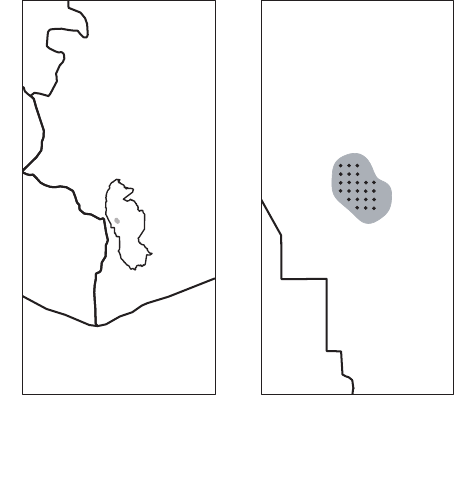
We used point transect DS methods to estimate the density of

Maxwell’s duikers within the territory of the ‘east group’ habituated

chimpanzee community in Ta

€

ı National Park, C

ote d’Ivoire

(Despr



es-Einspenner et al. 2017; Fig. 1a). Maxwell’s duikers were

sampled from 28 June through 21 September 2014 at 23 camera traps

(Bushnell Trophy Cam

; Bushnell, Overland Park, MO, USA,

Model 119576C) mounted at a height of 07–10 m and set to high

sensitivity. Cameras were deployed with a ﬁxed orientation of 0˚ at

the intersections of a grid with 1 km spacing and a random origin

superimposed over the study area (Fig. 1b). Realised sampling loca-

tions and orientations deviated from the design by as much as 30 m,

and 40°, respectively, in order to mount cameras on trees and to

ensure there was some chance of detecting animals. During installa-

tion of each camera, we measured horizontal radial distances from

the camera, and recorded videos of researchers holding distance

markers, at 1 m intervals out to 15 m, in the centre and along both

sides of the FOV. We estimated distances to ﬁlmed duikers by com-

paring their locations to those of researchers in the reference videos.

We set t = 2 s, and recorded the distance interval within which the

midpoint of each animal fell at 0, 2, 4, ..., 58 s after the minute. Lar-

ger distances were more diﬃcult to measure precisely, so we assigned

animals to 1-m intervals out to 8 m, but binned observations between

8 and 10 m, 10 and 12 m, 12 and 15 m, and beyond 15 m.

We excluded data from one camera because the FOV was lar-

gely obscured by vegetation, and another which was placed on a

slope and failed to detect any animals, but we included data from

a third camera that functioned normally but did not detect any

duikers. Maxwell’s duikers sleep or rest for most of each night and

for shorter periods during the day (Newing 1994, 2001). We

assumed they would not be available for detection overnight and

excluded the hours of darkness (19.00–6.00 h) from T

apriori.

We accounted for limited availability during the daytime three dif-

ferent ways. First we naively assumed that all duikers were active

by 6.30.00 h and remained so through 17.59.59 h, included dis-

tances observe d du ring this interval in a ‘daytime’ dataset, and

deﬁned temporal eﬀort at each locatio n (T

/t) as the number of 2-s

time steps during that time interval (20 699), multiplied by the num-

ber of sampling days. Second, we assumed that all animals were

available only during apparent times of peak activity (6.30.00–

8.59.59 h and 16.00.00–17.59.59 h) and recalculated temporal eﬀort

and censored distance observations accordingly (T

/t per

day = 8098). Third, we deﬁned T

and included observations as

8·5°W8°W 7·5°W

7°W

6·5°W6°W

4°N

5°N6°N

°N

8°N

Liberia

Cote d'Ivoire

TNP

(a)

7·35°W7·3°W7·25°W

7·2°W

5·7

5·8°

5·9°

(b)

Fig. 1. Location of the study area (grey polygon) in Ta

€

ı National Park

(TNP), C

ote d’Ivoire, 2014 (a), and (b) locations of 23 camera traps

deployed in a grid with 1 km spacing within the study area.

Distance sampling with camera traps 3

above for the daytime dataset, and included an independent esti-

mate of the proportion of time captive Maxwell’s duikers were

active during the same time interval (064; Newing 2001) in the

denominator of eqn 2. We included only data from complete days

when cameras were operating and not visited by researchers.

We ﬁt point transect models in program Distance (version 7.0;

Thomas et al. 2010), deﬁning survey eﬀort at each location as

2pt

ThecamerashadanAOVof42°, and a wider eﬀective angle of

the sensor (Trailcampro.com 2015), so we set h = 42° or 0733

radians. We considered models of the detection function with the

half-normal key function with 0, 1 or 2 Hermite polynomial

adjustment terms, the hazard rate key function with 0, 1, or 2

cosine adjustments, and the uniform key function with 1 or 2

cosine adjustments. Adjustment terms were constrained, where nec-

essary, to ensure the detection function was monotonically decreas-

ing. We selected among candidate models of the detection function

by comparing AIC values, acknowledging the potential for overﬁt-

ting because many observations were not independent. We present

measures of uncertainty derived from design-based variances (‘P2’

of Fewster et al. 2009, Web Appendix B), and from 999 bootstrap

resamples, with replacement, across camera locations.

Results

SIMULATIONS

Where we used the simple model of animal movemen t, and

where we used the complex model of animal movement and

collected data only when animals were active,

D was unbi-

ased (Table S1). Results were biased and erratic when we

recorded distances to resting animals (see Appendix S1 for

details). Design-based variances were smaller than the sam-

pling variance of

D across iterations, and associated conﬁ-

dence interval coverage was <90% (Table S1). Where we

estimated variance by bootstrapping, the coeﬃcient of vari-

ation was 0119, similar to the sampling variance of

D,and

CI coverage was 936% across 1000 iterations. Doubling

spatial sampling eﬀort improved precision, slightly more so

where we doubled the number of locations as opposed to h

(Table S1).

EXAMPLE: MAXWELL’S DUIKERS IN TA

€

INATIONAL PARK

We obtained 11 324 observations of the distance between

Maxwell’s duikers and cameras in 806 diﬀerent videos. Duik-

ers were rarely ﬁlmed during hours of darkness, and none were

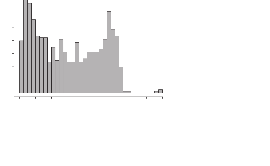
ﬁlmed between midnight and 6.00 h. The frequency of detec-

tion increased steadily after 6.00 h to a maximum between

6.30 h and 7.00 h and remained relatively high until 9.30 h,

after which it decreased slightly and remained relatively low

until16.30h,thenincreasedagainandremainedhighuntil

18.00 h, then declined gradually until 19.00 h (Fig. 2). Duikers

were always active when detected; CTs did not record any

duikers that were asleep or stationary for an entire minute. We

recorded 11 180 distances from 6:30:00 h through 17:59:59 h,

and 6274 during times of peak activity.

Exploratory analyses revealed no evidence of data collection

errors, and a paucity of observations between 1 and 2 m but

not between 2 and 3 m, so we left-truncated at 2 m. Fitted

detection functions and probability density functions were

heavy-tailed when distances >15 m were included, so we right-

truncated at 15 m. Truncating removed 8% of observations

from the daytime dataset, leaving n = 10 284, and 65% of

observations from the peak activity dataset, leaving n = 5865.

Mean encounter rates (mean numbers of duikers observed per

2-s time interval) across all points were 327 9 10

4

during the

daytime and 476 9 10

4

during times of peak activity.

Encounter rates were highly variable among locations but did

not exhibit an obvious spatial pattern across the study area,

and there was no evidence of spatial autocorrelation

(Moran’s I P = 047; Fig. 3).

When we ﬁt the hazard rate model with two adjustment

terms to the daytime dataset, the detection function was not

monotonically decreasing, so this model was not considered

for estimation. All models were ﬁtted successfully to the peak

activity dataset. The hazard rate model with no adjustments

minimised AIC and was used to estimate density in both cases.

Probability density functions of observed distances and rela-

tionships between detection probability and distance were sim-

ilar (Fig. 4). Detection probability was ~10within5mand

0·02 0·04 0·06 0·08 0·10 0·12

6:00 8:00 10:00 12:00 14:00 16:00 18:00 20:00 22:00 24:00

Time

Denstiy of video start times

Fig. 2. Histogram of start times of videos of

Maxwell’s duikers in Ta

€

ı National Park, C

ote

d’Ivoire, 2014.

4 E. J. Howe et al.

005 at 15 m; eﬀective detection radii were 91and94mfrom

the daytime and peak activity datasets, respectively.

We expected to underestimate density where we assumed

duikers were active all da y;

D was 37% higher when we

included only data from times of peak activity (Table 1).

Including an independe nt estimate of the proportion of time

active during the daytime as a parameter in the model ﬁt to the

daytime dataset yielded a still higher estimate (‘Active daytime’

in Table 1). Measures of uncertainty in the proportion of time

active were not available (Newing 2001) so did not contribute

to the variance of

D. Bootstrap variances were larger than

design-based analytic variances (Table 1). The vast majority

(998%) of the design-based variance of

D was attributable to

the variation in encounter rate between locations, and only

02% to detection probability.

Discussion

Simulations demonstrated the potential for the method to yield

unbiased density estimates, but also that animals’ activity pat-

terns must be accounted for. Where simulated animals rested

for half of each day and we set T

equal to the survey duration,

the most common scenario was that animals did not rest in

frontofCTsandnegativebiasin

D was proportional to the

time spent resting. When we recorded distance at each snap-

shot moment while animals rested in front of CTs, the encoun-

ter rate and therefore

D washigheronaverage,buttheshape

of the detection function was strongly aﬀected, leading to erra-

tic estimates and cases where models could not be ﬁtted to the

data. In practice, it is unlikely that we would detect animals

while they sleep or rest because movement will be insuﬃcient

to trigger the sensor. Therefore, estimates of the proportion of

time animals are active within the vertical range of CTs will be

required to avoid negatively biased

D. Ideally, this proportion

would be estimated from data collected concurrently with the

distance data to ensure it is representative. Fortunately, the

temporal distribution of camera trap detections is informative

Fig. 3. Variation in encounter rates of Maxwell’s duikers among 21

camera trap locations in Ta

€

ı National Park, C

ote d’Ivoire, 2014 (range

000–145 9 10

3

). The areas of the grey circles are proportional to the

encounter rates.

0 5 10 15

0·00 0·05 0·10 0·15

Daytime

Probability density

0 5 10 15

0·00 0·05 0·10 0·15

Peak activity

0 5 10 15

0·0

0·40·8

1·2

Detection probability

Distance

0 5 10 15

0·00·40·81·2

Distance

Fig. 4. Probability density functions of

observed distances (top) and detection proba-

bility as a function of distance (bottom) from

hazard-rate point transect models ﬁt to data

from Maxwell’s duikers in Ta

€

ı National Park,

2014 collected during the daytime (left) and

during times of peak activity (right).

Distance sampling with camera traps 5

regarding animal activity patterns (Lynam et al. 2013; Cruz

et al. 2014; Rowcliﬀe et al. 2014). If it is reasonable to assume

that the entire population is available for detection for any part

of each day, additional data would not be required to estimate

D accurately, because we could either (i) analyse only the data

collected at that time, censoring eﬀort and distance data from

other times, or (ii) estimate the overall proportion of time

active directly from the CT data (e.g. Rowcliﬀe et al. 2014).

Newing’s (1994) data from Ta

€

ı indicated that there was no time

at which all wild duikers could be assumed to be active. If this

was true during our survey, we may have underestimated den-

sity where we did not correct for limited availability within the

time included in T

, because even at times of peak activity some

animals may have been resting and unavailable for detection.

Activity data from wild duikers were presented only as ﬁgures

and could not be converted into estimates of the overall pro-

portion of time active (Newing 1994). We therefore relied on

the assumption that activity data from captive duikers (New-

ing 1994, 2001) were representative of activity patterns during

our survey. If this assumption held, then the density estimate

calculated using their estimate of the proportion of time active

during the day should not be biased as a result of limited avail-

ability. We suggest that the need to account for availability

should not pose a serious obstacle to reliable estimation of the

density of many species, but for others, notably ectotherms,

and semi-arboreal and fossorial species, it will require careful

consideration, and possibly additional data. We further sug-

gest that combining Rowcliﬀe et al.’s (2014) or similar meth-

ods for estimating the proportion of time active from detection

times at CTs with the point transect method described here

could yield accurate density estimates for many species from

CT data alone.

Avoidance of, or attraction to, CTs would bias encounter

rates and therefore density estimates. Some species exhibit

complex responses to CTs or are particularly wary of humans



equin et al. 2003). If behavioural responses are expected or

apparent in images of detected animals, CTs could be deployed

prior to the start of the actual survey to allow animals to

become accustomed to them and for signs of human presence

to dissipate. Similarly, eﬀort and distance data from times

when animals may have been displaced from the trap sites by

humans visiting them to download data, replace batteries, etc.,

should be censored.

The probability of detection at PIR CTs is lower at greater

angles from the centre of the FOV, due to a combination of the

trigger speed, the eﬀective horizontal angle of the sensor rela-

tive to the AOV of the camera (which varies among CT mod-

els) and possibly reduced sensitivity of the sensor at the

periphery of its horizontal range (Rowcliﬀe et al. 2011; Rovero

et al. 2013; Rovero & Zimmermann 2016). This introduces

heterogeneity in the detection function. Fortunately, provided

that detection is certain at the zero distance, the pooling robust-

ness property ensures that estimation is unbiased in the pres-

ence of heterogeneity in detectability among individuals

(Buckland et al. 2004),andthisalsoappliestoheterogeneity

caused by diﬀerences in angle at diﬀerent snapshot moments.

However, if detection probability at high h is much lower than

in the centre, ﬁtted models of the detection function might

show a rapid drop in detection probability near the point,

whereas detection functions with a gradual decrease near the

point are preferred for stable density estimation (Buckland

et al. 2001). The expected distribution of angles within a sector

within which the sensor is fully eﬀective is uniform. We recom-

mend that researchers measure angles as well as distances to

detected animals (e.g. Caravaggi et al. 2016), and test for

departures from the uniformity assumption at increasing

angles as part of their exploratory analysis. If departures are

apparent, the data could be truncated to exclude observations

beyond an angle within which the distribution is approximately

uniform, in which case h should be set to two times the trunca-

tion angle rather than the AOV of the camera in the deﬁnition

of eﬀort. An alternative approach that would allow us to retain

all of the data would be to develop a two dimensional detection

function where detection probability depends on both radial

distance and angle from centre, using methods similar to those

developed by Marques et al. (2010). We expect heterogeneity

withangletobemoreseverewithCTmodelswithnarrowhori-

zontal ranges of the sensor relative to the AOV of the camera,

or slow trigger speeds, and where faster-moving animals are

sampled. CTs with fast trigger speeds, short recovery times,

and curved array Fresnel lenses (which provide a wide eﬀective

angle of detection such that the camera begins recording

images as or even before the animal enters the FOV; Rovero &

Zimmermann 2016) could reduce or eliminate diﬀerences in

detection probability at diﬀerent angles in future studies.

The encounter rate variance accounted for the vast majority

of the design-based variance in duiker density, and variances

around

D were larger than for simulated data despite similar

sample sizes. Real populations exhibit clumped or patchy dis-

tributions and non-random movement, leading to variable

encounter rates among sampling locations and hence greater

uncertainty in

D (Buckland et al. 2001; Fewster et al. 2009);

the small area sampled at each location exacerbates this prob-

lem. Increasing the area sampled will therefore enhance preci-

sion, more so than would increasing temporal eﬀort at a point.

Theory predicts that increasing the number of points will yield

the largest improvements to precision (Buckland 1984; Fewster

et al. 2009). That the improvement in precision in simulations

was only slightly greater where we doubled the number of sam-

pling locations than where we doubled h is not representative

Table 1. Densities of Maxwell’s duikers in Ta

€

ı National Park, 2014,

estimated using diﬀerent methods to account for limited availability for

detection

Design-based Bootstrap

Availability

D CV 95% CI CV 95% CI

Daytime 106027 61– 183040 50– 218

Peak activity 14 5030 78– 269036 61– 269

Active daytime 165027 95– 286040 77– 341

Bootstrap conﬁdence intervals were calculated using the percentile

method.

6 E. J. Howe et al.

of real studies because the expected spatial distribution of ani-

mal locations was uniform, and movement was random. Coef-

ﬁcients of variation around

D for duikers were >35% despite

large samples of distance observations, so we recommend that

future studies employ more points to improve precision.

The average density of Maxwell’s duikers throughout Ta

€

National Park was recently estimated as 16perkm

from line

transect DS surveys (N’Goran 2006). However, line transect

sampling by human observers is believed to severely underesti-

mate densities of forest-dwelling animals in general, and forest

antelopes in particular, due to eﬀects of evasive movement and

behaviour in response to observers on both the encounter rate

and the distribution of observed distances (Koster & Hart 1988;

Jathanna, Karanth & Johnsingh 2003; Rovero & Marshall

2004, 2009; N’Goran 2006; Marshall, Lovett & White 2008;

Marini et al. 2009). For this reason, line transect surveys of sign

are frequently performed, and sign densities converted to ani-

mal densities. This approach is expected to yield biased esti-

mates in the absence of local and concurrent estimates of sign

production and decay rates, which are time-consuming to esti-

mate (Plumptre 2000; Kuehl et al. 2007; Todd et al. 2008).

Dung surveys may further require genetic analysis to identify

the species (Bowkett et al. 2009). Distance sampling with CTs

apparently avoided the underestimation characteristic of line

transect surveys of live animals, in less time than would be

required to obtain reliable estimates from sign surveys.

The recent proliferation of CT studies is providing new

information about wildlife in diverse habitats (Burton et al.

2015; Rovero & Zimmermann 2016). Where estimating the

density of a rare but individually identiﬁable species is the pri-

mary research objective, it may be preferable to deploy CTs

non-randomly in order to obtain suﬃcient detections of indi-

viduals to estimate density by SECR (Wearn et al. 2013;

Cusack et al. 2015b; Despr



es-Einspenner et al. 2017). How-

ever, multiple research objectives can be addressed, and useful

data for multiple species obtained, if CTs are deployed

according to a randomised design (MacKenzie & Royle 2005;

Wearn et al. 2013; Burton et al. 2015; D



enes, Silveira & Beis-

singer 2015). The size of unmarked populations can then be

estimated from CT data, using Poisson and negative binomial

GLMs or hierarchical N-mixture models (D



enes, Silveira &

Beissinger 2015), but population density is of greater interest

because it is more biologically relevant and comparable across

studies. Densities of unmarked animal populations can only

be estimated from CT data using SECR models for unmarked

populations, the REM, or DS methods; the latter two require

randomised designs (Buckland et al. 2001; Rowcliﬀe et al.

2008). SECR methods for unmarked populations require

intensive designs, and even then estimates will often be too

imprecise to be useful unless a subset of the population can be

reliably identiﬁed (Chandler & Royle 2013; Saout et al. 2014).

The REM requires an estimate of the average speed of animal

movement, assumes that detection is certain within an estim-

able area in front of the camera, and makes use of only one

observation from each detected animal (Rowcliﬀe et al.

2008). Our point transect approach requires an estimate of

the proportion of time animals are available for detection,

assumes that detection is certain only at zero distance, and

multiple observations from each detected animal inform

detection probability estimates. We expect the extension of

point transect DS methods to provide an eﬀective and eﬃ-

cient tool for estimating animal density and to enhance the

information derived from CT surveys.

Authors’ contributions

E.J.H. contributed to the development of the point transect model for camera

traps, performed the analyses, and wrote the manuscript. S.T.B. conceived and

formulated the original version of the point transect model for camera traps, and

contributed to the manuscript text. M.-L.D.-E. helped to design and conducted

the ﬁeld study, estimated distances to Maxwell’s duikers from video footage,

wrote portions of the methods section, and contributed to the manuscript text.

H.S.K. designed the ﬁeld study and contributed to the manuscript text.

Acknowledgements

We thank the Robert Bosch Foundation, the Max Planck Society and the Univer-

sity of St Andrews for funding, the Minist



ere de l’Enseignement Sup



erieur et de la

Recherche Scientiﬁque and the Minist



ere de l’Environnement et des Eaux et For-

ets in C

ote d’Ivoire for permission to conduct ﬁeld research in Ta

€

ı National Park,

and Dr. Roman Wittig for permitting data collection in the area of the Ta

€

Chimpanzee Project.

Data accessibility

The data ﬁles from which densities of Maxwell’s duikers were estimated using

Distance software, and data describing start times of videos of Maxwell’s duikers,

have been archived at the Dryad data repository (https://doi.org/10.5061/dryad.

b4c70) (Howe et al. 2017).

References

Balestrieri, A., Ruiz-Gonz



alez, A., Vergara, M., Capelli, E., Tirozzi, P., Alﬁno,

S., Minuti, G., Prigioni, C. & Saino, N. (2016) Pine marten density in lowland

riparian woods: a test of the random encounter model based on genetic data.

Mammalian Biology-Zeitschrift f

€

ur S

€

augetierkunde, 81,439–446.

Bowkett, A.E., Plowman, A.B., Stevens, J.R., Davenport, T.R. & van Vuu-

ren, B.J. (2009) Genetic testing of dung identiﬁcation for antelope sur-

veys in the Udzungwa Mountains, Tanzania. Conservation Genetics, 10,

251–255.

Buckland, S.T. (1984) Monte Carlo conﬁdence intervals. Biometrics, 1, 811–817.

Buckland, S.T., Anderson, D.R., Burnham, K.P., Laake, J.L., Borchers, D.L. &

Thomas, L. (2001) Introduction to Distance Sampling: Estimating Abundance

of Biological Populations. Oxford University Press, Oxford, UK.

Buckland, S.T., Anderson, D.R., Burnham, K.P., Laake, J.L., Borchers, D.L. &

Thomas, L. (2004) Advanced Distance Sampling: Estimating Abundance of

Biological Populations. Oxford University Press, Oxford, UK.

Buckland, S.T., Rexstad, E.A., Marques, T.A. & Oedekoven, C.S. (2015) Dis-

tance Sampling: Methods and Applications. Springer, Heidelberg, Germany.

Burton,A.C.,Neilson,E.,Moreira,D.,Ladle, A., Steenweg, R., Fisher, J.T.,

Bayne, E. & Boutin, S. (2015) REVIEW: wildlife camera trapping: a review

and recommendations for linking surveys to ecological processes. Journal of

Applied Ecology, 52,675–685.

Caravaggi, A., Zaccaroni, M., Riga, F., Schai-Braun, S.C., Dick, J.T., Mont-

gomery, W.I. & Reid, N. (2016) An invasive-native mammalian species

replacement process captured by camera trap survey random encounter mod-

els. Remote Sensing in Ecology and Conservation, 2,45–58.

Chandler, R.B. & Royle, J.A. (2013) Spatially explicit models for inference about

density in unmarked or partially marked populations. The Annals of Applies

Statistics, 7, 936–954.

Cruz, P., Paviolo, A., B



o, R.F., Thompson, J.J. & Di Bitetti, M.S. (2014) Daily

activity patterns and habitat use of the lowland tapir (Tapirus terrestris)inthe

Atlantic Forest. Mammalian Biology-Zeitschrift f

€

ur S

€

augetierkunde, 79,376–

383.

Cusack, J.J., Dickman, A.J., Rowcliﬀe, J.M., Carbone, C., Macdonald, D.W. &

Coulson, T. (2015b) Random versus game trail-based camera trap placement

Distance sampling with camera traps 7

strategy for monitoring terrestrialmammalcommunities.PLoS ONE, 10,

e0126373.

Cusack, J.J., Swanson, A., Coulson, T., Packer, C., Carbone, C., Dickman, A.J.,

Kosmala, M., Lintott, C. & Rowcliﬀe, J.M. (2015a) Applying a random

encounter model to estimate lion density from camera traps in Serengeti

National Park, Tanzania. The Journal of Wildlife Management, 79, 1014–1021 .



enes, F.V., Silveira, L.F. & Beissinger, S.R. (2015) Estimating abundance of

unmarked animal populations: accounting for imperfect detection and other

sources of zero inﬂation. Methods in Ecology and Evolution, 6, 543–556.

Despr



es-Einspenner, M.-L., Howe, E.J., Drapeau, P. & K

€

uhl, H.S. (2017) An

empirical evaluation of camera trapping and capture-recapture methods for

estimating chimpanzee density. American Journal of Primatology, https://doi.

org/10.1002/ajp.2264 7

Eﬀord, M.G., Borchers, D.L. & Byrom, A.E. (2009) Density estimation by spa-

tially explicit capture – recapture: likelihood-based methods. Modelling Demo-

graphic Processes in Marked Populations (eds D.L. Thompson, E.G. Cooch &

M.J. Conroy), pp. 255–269. Springer, New York, NY, USA.

Fewster, R.M., Buckland, S.T., Burnham, K.P., Borchers, D.L., Jupp, P.E.,

Laake, J.L. & Thomas, L. (2009) Estimating the encounter rate variance in dis-

tance sampling. Biometrics, 65, 225–236.

Howe, E.J., Buckland, S.T., Despr



es-Einspenner, M.-L. & K

€

uhl, H.S. (2017)

Data from: Distance sampling with camera traps. Dryad Digital Repository,

https://doi.org/10.5061/dryad.b4c70

Jathanna, D., Karanth, K.U. & Johnsingh, A.J.T. (2003) Estimation of large her-

bivore densities in the tropical forests of southern India using distance sam-

pling. Journal of Zoology, 261, 285–290.

Koster, S.H. & Hart, J.A. (1988) Methods of estimating ungulate populations in

tropical forests. African Journal of Ecology, 26, 117–126.

Kuehl, H.S., Todd, A., Boesch, C. & Walsh, P.D. (2007) Manipulating decay time

for eﬃcient large-mammal density estimation: gorillas and dung height. Eco-

logical Applications, 17, 2403–2 414.

Laake, J.L., Collier, B.A., Morrison, M.L. & Wilkins, R.N. (2011) Point-based

mark-recapture distance sampling. Journal of Agricultural, Biological, and

Environmental Statistics, 16, 389–

408.

Lynam, A.J., Jenks, K.E., Tantipisanuh, N. et al. (2013) Terrestrial activity pat-

ternsofwild cats from camera-trapping.Raﬄes Bulletin of Zoology, 61,407–415.

MacKenzie, D.I. & Royle, J.A. (2005) Designing occupancy studies: general

advice and allocating survey eﬀort. Journal of Applied Ecology, 42, 1105–1114.

Marini, F., Franzetti, B., Calabrese, A., Cappellini, S. & Focardi, S. (2009)

Response to human presence during nocturnal line transect surveys in fallow

deer (Dama dama) and wild boar (Sus scrofa). European Journal of Wildlife

Research, 55, 107–115.

Marques, T.A., Buckland, S.T., Borchers, D.L., Tosh, D. & McDonald, R.A.

(2010) Point transectsamplingalong linear features. Biometrics,66, 1247–1255.

Marques, T.A., Thomas, L., Fancy, S.G. & Buckland, S.T. (2007) Improving esti-

mates of bird density using multiple-covariate distance sampling. The Auk,

124, 1229–1243.

Marshall, A.R., Lovett, J.C. & White, P.C.L. (2008) Selection of line-transect

methods for estimating the density of group-living animals: lessons from the

primates. American Journal of Primatology, 70,452–462.

Miller, D.L. 2015. Distance: distance sampling detection function and abundance

estimation. R package version 0.9.4. http://CRAN.R-project.org/package=

Distance (accessed 9 November 2016).

Newing, H.S. 1994. Behavioural ecology of duikers (Cephalophus spp.) in forest

and secondary growth, Ta

€

ı, C

ote d’Ivoire. PhD thesis, University of Stirling,

Stirling, Scotland.

Newing, H.S. (2001) Bushmeat hunting and management: implications of duiker

ecology and interspeciﬁc competition. Biodiversity and Conservation, 10,

99–118.

N’Goran, P.K. 2006 Quelques r



esultats de la premi



ere phase du biomonitoring

au Parc National de Ta

€

ı(ao

ut 2005 – mars 2006). Ministere de l’Environ-

nement et des Eaux et Forets, Ministere de l’Enseignement Superieur et de la

Recherce Scientiﬁque, Abidjan, C

ote d’Ivoire.

Plumptre, A.J. (2000) Monitoring mammal populations with line transect tech-

niques in African forests. Journal of Applied Ecology, 37, 356

–368.

Rovero, F. & Marshall, A.R. (2004) Estimating the abundance of forest antelopes

by line transect techniques: a case from the Udzungwa Mountains of Tanza-

nia. Tropical Zoology, 17,267–277.

Rovero, F. & Marshall, A.R. (2009) Camera trapping photographic rate as an

index of density in forest ungulates. Journal of Applied Ecology, 46,1011–1017.

Rovero, F. & Zimmermann, F. (2016) Camera Trapping for Wildlife Research.

Pelagic Publishing, Exeter, UK.

Rovero, F., Zimmermann, F., Berzi, D. & Meek, P. (2013) ‘Which camera trap

type and how many do I need?’ A review of camera features and study designs

for a range of wildlife research applications. Hystrix, the Italian Journal of

Mammalogy, 24, 148–156.

Rowcliﬀe, M.J., Carbone, C., Jansen, P.A., Kays, R. & Kranstauber, B. (2011)

Quantifying the sensitivity of camera traps: an adapted distance sampling

approach. Methods in Ecology and Evolution, 2,464–476.

Rowcliﬀe, J.M., Field, J., Turvey, S.T. & Carbone, C. (2008) Estimating animal

density using camera traps without the need for individual recognition. Journal

of Applied Ecology, 45, 1228–123 6.

Rowcliﬀe, J.M., Jansen, P.A., Kays, R., Kranstauber, B. & Carbone, C. (2016)

Wildlife speed cameras: measuring animal travel speed and day range using

camera traps. Remote Sensing in Ecology and Conservation, 2,84–94.

Rowcliﬀe, M.J., Kays, R., Kranstauber, B., Carbone, C. & Jansen, P.A. (2014)

Quantifying levels of animal activity using camera trap data. Methods in Ecol-

ogy and Evolution, 5, 1170–1179.

Saout, S.L., Chollet, S., Chamaill



e-Jammes, S. et al. (2014) Understanding the

paradox of deer persisting at high abundance in heavily browsed habitats.

Wildlife Biology, 20, 122–135.



equin, E.S., Jaeger, M.M., Brussard, P.F. & Barrett, R.H. (2003) Wariness of

coyotes to camera traps relative to social status and territory boundaries.

Canadian Journal of Zoology, 81,2015–2025.

Sollmann, R., Mohamed, A. & Kelly, M.J. (2013a) Camera trapping for the study

and conservation of tropical carnivores. The Raﬄes Bulletin of Zoology, 28,

21–42.

Sollmann, R., Mohamed, A., Samejima, H. & Wilting, A. (2013b) Risky business

or simple solution – relative abundance indices from camera trapping. Biologi-

cal Conservation, 159, 405–412.

Thomas, L., Buckland, S.T., Rexstad, E.A., Laake, J.L., Strindberg, S., Hedley,

S.L., Bishop, J.R.B., Marques, T.A. & Burnham, K.P. (2010) Distance soft-

ware: design and analysis of distance sampling surveys for estimating popula-

tion size. Journal of Applied Ecology, 47,5–14.

Todd, A.F., Kuehl, H.S., Cipolletta, C. & Walsh, P.D. (2008) Using dung to esti-

mate gorilla density: modeling dung production rate. International Journal of

Primatology, 29, 549–563.

Trailcampro.com (2015) Available at: http://www.trailcampro.com/ (accessed 5

August 2015).

Wearn, O.R., Rowcliﬀe, J.M., Carbone, C., Bernard, H. & Ewers, R.M. (2013)

Assessing the status of wild felids in a highly-disturbed commercial forest

reserve in Borneo and the implications for camera trap survey design. PLoS

ONE, 8, e77598.

Zero, V.H., Sundaresan, S.R., O’Brien, T.G. & Kinnaird, M.F. (2013) Monitor-

ing an Endangered savannah ungulate, Grevy’s zebra Equus grevyi:choosinga

method for estimating population densities. Oryx, 47, 410–419.

Received 13 January 2017; accepted 15 March 2017

Handling Editor: Jason Matthiopoulos

Supporting Information

Details of electronic Supporting Information are provided below.

Appendix S1. MEE-17-01-032-S1 describes simulation methods and

results in detail.

8 E. J. Howe et al.