
Barclays PLC
Corporate Transition
Risk Forecast Model
2021

Contents
Inside this book
Introduction
01
1 Input Data
02
2 Assessment
05
3 Financial and Credit Risk Outputs
16
4 Known Enhancements
22

Scenario analysis plays an important role in
assessing the future implications of potential
climate change pathways on Barclays’, and is a
key part of the organization’s approach to
climate risk management.
If the transition to a low-carbon economy
happens too slowly, climate change could have
devastating eects on our planet. If the
transition is disorderly, there could be very real
social and economic costs for families and
businesses around the world – from
unemployment and nancial hardship, to
insucient food and fuel to meet their daily
needs. We must weigh and balance those risks in
order to maximise our contribution to
addressing the climate challenge.
Against this backdrop is an evolving regulatory
landscape, with many regulators increasing
theiroversight and expectations of climate risk
management in recent years. In 2019, Barclays’
principal regulator, the PRA, published a
Supervisory Statement outlining requirements
for a strategic approach to the management
ofthe nancial risks posed by climate change.
These were enhanced in July 2020, setting a
deadline for implementation of end2021.
Central Banks and regulators are also
increasingly engaging in supervisory stress
teststo understand the climate vulnerabilities
ofparticipants, including the Bank of France/
French Prudential Supervision and Resolution
Authority, the Netherlands Bank (DNB), the
Bankof England and the Prudential Regulation
Authority, and the European Central Bank.
Climate change is a global and pervasive risk
andopportunity to companies and there will
inevitably be winners and losers across all
sectors. Assessing this impact requires new
approaches and tools, which consider both
climate, macro-economic and sector and
company specic factors. Barclays started
assessing those impacts in 2018, initially
qualitatively and has since aimed to create
quantitative methodologies for several of its
keyportfolios. These new approaches and
toolsfocus on company level analysis,
whichdiers from more traditional stress
testingexercises, conducted at portfolio or
sector level, as a counterparty unit of analysis
better captures the novel risk driver’s climate
change presents. To support this, Barclays
developed a methodology to assess the impacts
of future climate transition scenarios on
corporate companies from economic sectors
that Barclays considers to besubject to elevated
climate risk (as dened in our TCFD report). This
methodology produces revised future nancial
metrics impacted by such scenarios, which can
in turn be used in credit risk assessments.
This methodology is rst generation and is
focused on capturing the directionality and
magnitude of climate change impacts to
companies, rather than achieving a high degree
of accuracy. Over time it is expected that this
approach will evolve and be rened as data
availability improves and methodological
techniques are rened. This whitepaper is
shared in this spirit, to add to the growing body
of literature on how to assess the risks arising
from climate change, to invite feedback and to
support other actors in developing their
approaches to this eld.
The key design principles of the methodology
are outlined below, across the input data
required, the assessment performed and
theresulting nancial and credit impacts.
Greater detail is included in subsequent
sectionsoutlining how each of these steps
isoperated and integrated into the overall
methodological approach.
Introduction
1. Input Data 3. Financial and Credit Risk Impact2. Assessment
Financial Impact
■
Forecast future revenue, gross prots,
earnings and net debt
Credit Scorecard
■
Assess 3 factors:
– Size
– Protability
– Leverage
Downstream models
■
Climate adjusted future credit rating
Adaptation
■
Actions to mitigate climate risks
■
Impacts to revenues and emissions
■
CapEx from shift in low/high
carbonactivities
Carbon Costs
■
Carbon tax from GHG emissions
■
% carbon costs passed to
nextconsumer
Gross Prot
■
Changing prices for fossil fuels
■
Changing demand for goods and
services on revenue and costs
Scenario Variables
■
Commodity demand and prices
■
Low/high carbon product demand
■
Carbon prices
Company Data
■
Revenue, costs and earnings
■
Net debt
■
GHG emissions
Internal Credit Metrics
■
Credit ratings (Default Grade)
■
Exposure at default
■
Loss given default
Barclays PLC
home.barclays/annualreport 01
Barclays PLC Corporate Transition Risk Forecast Model 2021

1.1 Scenarios
The purpose of the methodology is to calculate
future company level nancial and credit metrics,
impacted by the climate specic transition
scenario being assessed. To that end, it is
capable of consuming a wide range of scenarios
depending on the objective of the assessment.
It has in particular been designed to utilise
scenarios developed by the Bank of England in
the context of its 2021 Climate Biennial
Exploratory Scenario (CBES) and by the Network
for Greening the Financial System (NGFS),
including Orderly and Disorderly transitions.
Whilst the methodology is capable of running
various transition scenarios, in order to support
the assessment granularity, the scenarios being
used should include a wide variety of demand
and price curves for commodities and products
and services. This includes for example, power
capacity, fossil fuels, transport capacities and
products such as cement and steel. Throughout
this report, NGFS scenarios are used to
demonstrate examples of the methodology,
specically the Orderly Net Zero 2050 scenario,
which informed the Bank of England’s Early
Action scenario. It is worth noting that Barclays
expanded certain scenario variables that were
not published.
1.2 Company Data
To perform granular assessments of the
impacts of future climate scenarios on
corporate companies, the methodology requires
detailed information on the company, including
i)nancial metrics, ii) emissions data and iii)
internal credit metrics. It is important that
relevant information about the company is
isolated as of today, to subsequently apply
theimpact of future climate scenario variables.
Obtaining data is challenging, across a number
of dierent dimensions including data sourcing,
granularity, and format. As a result, estimation
techniques and proxies are often required in
order to perform the assessment. The increase
in companies disclosing climate risk information
in TCFD reports has driven a signicant increase
in the number of data points available to perform
the assessment, in turn lowering the reliance
onestimations. This should increase the validity
of the assessments performed.
1.2.1 Company Financial Data
For nancial data, the corporate population is
segmented into dierent sectors according to
the principal business activity they perform.
Company’s activities are further attributed to
key sector specic technologies, according to
the revenues they generate from these
products/services. These technologies have
been chosen as they are deemed to be the most
important business segments impacted from a
climate change perspective. It is noted that
some companies operate across a multitude of
activities, and in the future the methodology
aims to make these technologies sector
agnostic so that revenues can be attributed to
any technology irrespective of the sector in
which the company operates. However, these
instances are small in number and in many cases
additional operations for companies within a
sector, not captured within the chosen
technologies, will face minimal impacts from
climate change. In such cases, increasing the
number of the possible technologies per sector
does not add additional analytical value. The
methodology currently treats these Revenues
as “Other” and holds these constant over the
scenario forecast.
This segmentation and attribution generates a
detailed picture of the companies’ starting
business model that can be used to forecast the
impact of scenario variables. The below table
demonstrates sectors and technologies
considered:
Technology
Type 1 Type 2 Type 3 Type 4 Type 5
Agriculture Crop Production Animal Production Trading
Automotive
Manufacturing
Internal Combustion
Engine
Hybrid Electric Vehicle
Aviation Air Travel
Cement Cement
Chemicals PetroChem Non-PetroChem
Coal Mining and
CoalTerminals
Coal Mining Other Mining
Mining Coal Mining Transition Metal
Mining
Other Mining
Oil & Gas Oil (Margin based) Gas (Margin Based) Oil (Production
based)
Gas (Production
Based)
Renewables
Power Utilities Coal Power Gas Power and
Distribution
Nuclear Power Renewable Power Electricity
Transmission and
Distribution
Road Haulage Road Haulage Logistics
Shipping Shipping Logistics
Steel Steel
1 Input Data
Barclays PLC
home.barclays/annualreport02
Barclays PLC Corporate Transition Risk Forecast Model 2021

As an example, for a company operating in the
Automotive Manufacturing sector, current
nancial performance is segmented into
revenues generated through the sale of internal
combustion engine (ICE), hybrid and electric
vehicles (EV). This enables a better
understanding of the company’s current
exposure to products and services that will
beimpacted by the transition to a low carbon
economy, in this case the increase in sales of
EVs versus the decline in the sale of ICE vehicles.
Those operating in this sector will be subject to
these demand shifts, which will in turn have a
knock on impact on revenues, whereby those
able to produce greater volume of EVs will be
better able to benet from the transition and
outperform peer competitors. Likewise, in the
Mining sector, companies with signicant coal
activity are likely to face more challenging
business environments than those with less, and
vice versa for companies with greater transition
metal activities.
The choice to focus on revenue generation as
the underlying performance metric represents a
key design choice, where revenue is used as a
substitute to modelling underlying production.
This is recognition of the cross-sector
application of this approach, and the lack of
readily available data on company’s performance
in terms of production, meaning that revenue
generation provides a consistent and reliable
metric on which to forecast future nancial
performance across sectors. The implication
within this is that margins associated with
production are both the same across
technologies within a sector and remain
constant over time, which given the long term
nature of these scenarios and dierentiation of
technologies within sectors, is in reality likely to
be variable. However, the ability to model such
changing margins is currently beyond the scope
of this methodology.
A number of data sources are used to
breakdown revenues by technology type. Such
data can be challenging to obtain, and certain
sectors are less prone to disclose revenue split
across these technologies. A waterfall
hierarchical approach is used to capture actual
revenue share data, or estimations with the
proportion of total revenue across technologies,
where this is not available.
Is company revenue share data available? S&P CAPIQ
Yes
No
Is company production data available? Asset Resolution
Yes
No
Do company disclosures include revenue
or production share data?
Company Disclosures
Yes
No
Sector Average
Barclays PLC
home.barclays/annualreport 03
Barclays PLC Corporate Transition Risk Forecast Model 2021
1.2.2 Company emissions data
The greenhouse gas emissions of corporate
companies, both current and future, also
represents a key metric when assessing the
future nancial impact of the transition to a low
carbon economy. As governments around the
world seek to reduce GHG emissions through
greater regulation, the resultant policy decisions
are likely to generate winners and losers
depending on how signicantly companies can
reduce their emissions footprint.
Data availability for company emissions is
continuously improving, as more companies
begin to disclose this information as well as
greater numbers of external third party providers
providing estimation methodologies. This
methodology combines both company level
disclosures where available and sector-level
estimate where not. These estimation
approaches are in line with the methodologies
taken by many leading third party vendor
approaches. It sums both the scope 1 and 2
emissions of companies, but does not capture
the direct impact of scope 3 emissions, as these
are assumed to be indirectly factored into the
demand shocks inherent in the scenario (see
section 2.1 for more detail).
Company disclosure data on emissions is used
as the primary source, noting that it is most likely
to represent the in-scope GHG emissions the
company would face under carbon pricing
regimes. Where this is not available, a two-step
estimation based on nancial intensity is used:
■
Calculate sectoral level nancial intensity
metrics, using revenues per tonne of carbon
dioxide equivalent emissions for companies
within those sectors.
■
For companies with missing emissions data,
multiply revenues by the nancial intensity
metric to obtain estimation of the company’s
emissions.
The above approach represents a simplifying
method for obtaining emissions estimates,
given that with nancial emissions intensities
within a sector may well deviate on a company by
company basis, as GHG emissions are driven by
alarge number of factors. One of its key benets
is that it can be implemented consistently
across a wide range of sectors, company sizes
and organisational types.
1.3 Internal Credit Metrics
The use of internal credit metrics such as
Default Grade (DG), Loss Given Default (LGD)
and Exposure at Default (EAD) is not required to
calculate nancial impacts to companies,
however this information is used when
translating future nancial impacts to credit
impacts. These data inputs are obtained from
existing internal credit systems. Barclays DG is
the internal credit metric used as part of
company credit assessment and provides an
integer representation of the probability of
default of a company from DG1 (least risky) to
DG22 (default). Further information on the
assessment of credit risk impact can be found in
section 3.2, and on Barclays DG scoring from
Barclays Pillar 3 report.
1 Input Data continued
Barclays PLC
home.barclays/annualreport04
Barclays PLC Corporate Transition Risk Forecast Model 2021

2 Assessment
2.1 Gross Prot Calculation
The methodology treats future scenario
impacts on nancial performance as a sensitivity
to a starting jump o point. In essence, the
calculation takes the attributed revenues to
each technology, and then calculates future
revenue by using the appropriate scenario
variable curve. For a hypothetical Mining
company, Coal Mining, Transition Metals Mining
and Other Mining are the technologies and the
demand curve for each of these products can
be applied to their starting revenues to indicate
future revenues. In some sectors, this general
approach has been further enhanced to include
sector specic assumptions and dynamics. This
currently covers Oil & Gas, Power Utilities and
Automotive sectors given their central role in the
transition to a low carbon economy. Further
sectors would likely benet from an enhanced
approach as well, and the intention is that the
methodology will evolve over time to include
these.
2.1.1 General Approach
The approach projects income statement and balance sheet line items by establishing a link between
the jump-o nancial statements and scenario variables.
For total revenue projections, the equation is given below.
TotalRevenue
t
=∑
s
s
[Δ
s,t
× Π
s,t
] × AllocatedRevenue
s,t
(1)
Where delta represents the demand scenario
variable and pi represents the price scenario
variable for technology s (values are rebased as a
ratio of the latest jump-o level).
AllocatedRevenue represents the jump-o
revenue in the forecast (the latest actuals
values), multiplied by the share of revenues a
company expects to generate from a given
technology as a fraction of its total revenues.
Implicit in this calculation is the assumption that,
absent of any companies within a sector
changing their business model, market share
would remain constant for all market participants
and that any increasing demand for goods and
services is met by rms. This is a simplication,
and incorporation of assumptions on the
interplay between market incumbents and new
entrants is currently being considered as an
additional module.
Cost of sales is modeled in a similar approach,
with the notable dierence that the market price
of each technology is not considered as a factor
for cost of sales. In other words, if the price of oil
falls in the market, then a given oil producer will
not incur decreasing cost of sales from its oil
production based on the lower market price.
Again, this is a simplication as it eectively
assumes that the cost per unit of production
remains static.
CostOfSales
t
=∑
s
s
[θ
s,t
× Δ
s,t
] × CostOfSales
t=0
(2)CostOfSales
t
=∑
s
s
[θ
s,t
× Δ
s,t
] × CostOfSales
t=0
(2)
Note that the formula for cost of sales is similar to that of (1), with the notable exception that pi does
not factor into the formula.
The net dierence between total revenues and cost of sales is dened as gross prots.
GrossProt
t
= TotalRevenue
t
− CostOfSales
t
(3)
This includes variable costs directly incurred
during the production of goods and services.
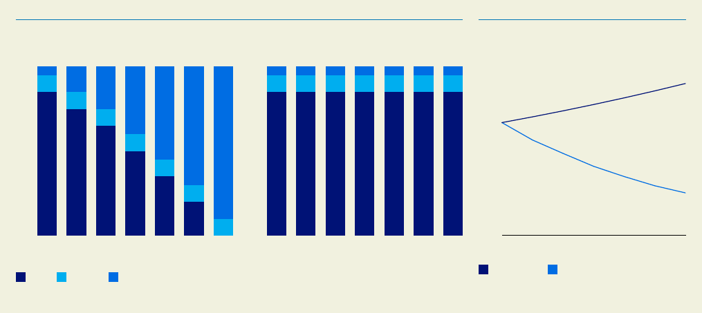
The below graph demonstrates a hypothetical
example for a Mining company, where the
dierence between two peer companies is only
the starting business operations split across
three technologies; Coal Mining, Transition
Metals Mining and Other Mining. Given the
dierence in the future demand for these
products, the fortunes of these two companies
will diverge over time should neither take steps
to evolve their business model.
Barclays PLC
home.barclays/annualreport 05
Barclays PLC Corporate Transition Risk Forecast Model 2021

In the below example, Company A generates
40% of its revenues from coal with only 20%
from transition metals, whereas Company B is
better positioned with half of its business
revenue generated from transition metals and
only 10% from coal. In both cases the remaining
percentage of revenue is from "Other Mining"
products, the demand for which is held at over
the scenario. As a result, Company B is well
placed to take advantage of the transition and
inturn grow its revenues substantially.
2 Assessment continued
Mining Commodity Demand
%
Company Revenues
£mn
2020 2025 2035 2045 20502030 2040
800
600
400
200
0
Thermal Coal Other Mining Transition Metals
2020 2025 2030 2035 2040 2045 2050 2020 2025 2030 2035
Company A Company B
2040 2045 2050
50,000
40,000
30,000
20,000
10,000
0
Thermal Coal Transition MetalsOther Mining
2.1.2 Oil & Gas Approach
Within this sector, revenue generation is split at a
more granular level, to reect two dierent
revenue types. The rst is where the Oil & Gas
products that drive the revenue have initially
been purchased by the company from a third
party. These products may then be sold on
immediately, for example in the case of Trading,
or where the company transforms the product in
some way before onward sale, for example in the
case of Rening. In this instance, it is assumed
that price dynamics in the scenario are less
material, as broadly prices going up/down will
aect both revenues and costs, and therefore
cancel one another out with respect to overall
nancial performance (eg. prot/earnings). In
contrast, revenue generation driven by raw Oil &
Gas products that have been developed by the
company themselves, for example Upstream
production, will be more sensitive to price
dynamics as falls/rises in price will impact
revenues more signicantly than costs.
For Oil & Gas (Margin Based) revenue, the
formula given in (1) is simplied as follows:
:
CostOfSales
t
=∑
s
s
[θ
s,t
× Δ
s,t
] × CostOfSales
t=0
(2)TotalRevenue
t
=∑
s
s
[Δ
s,t
] × AllocatedRevenue
s,t
(4)
For Costs, given the large reduction in oil & gas
consumption in transition scenarios, it is
reasonable to expect that companies would
seek to manage down their cost base and their
unit cost, for example by reducing production
from their most expensive elds rst. To reect
this, the methodology applies a scalar to reduce
cost of sales, with γ in the formula below
representing the cost eciency measures.
Theextent to which a company can reduce
these costs is calibrated based on the size of the
company as a proxy for the extent to which cost
eciencies can be made i.e. the larger the
company, the greater the cost eciency
improvements possible. For Oil & Gas Upstream
sector, the cost of sales formula given in (2) is
extended to the below.
CostOfSalesUpstream
t
= UpstrCostOfSales
t
× (1–1
t,scen
× y)
(5)
Barclays PLC
home.barclays/annualreport06
Barclays PLC Corporate Transition Risk Forecast Model 2021

2.1.3 Power Utility Approach
Power Utilities is an important sector for the transition, both because of the projected electrication
of the economy (leading to more electricity being consumed) and of the need to decarbonise the
electricity grids by switching technology types.
For Power Utilities, total revenues are projected by linking jump-o total revenues to the growth in
total electricity capacity. This contrasts to the general methodology where each technology is driven
by its own demand driver.
TotalRevenue
t
= Φ
ElectricityDemand,t
× TotalRevenue
t=0
(6)
Φ
ElectricityDemand,t
= ElectricityDemand
t
(7)
ElectricityDemand
t=2020
The break-out between polluting sources of
power and renewable sources of power is
dependent on the credibility of the company’s
adaptation plan (see section 2.3 for how
adaptation plans are assessed). For companies
with credible adaptation plans, total revenue
break-out will be based on the technology splits
given in the company’s adaptation plan, and
scaled by the growth in total electricity demand.
For companies with adaptation plans that are
not considered credible, the generation capacity
of polluting technologies will be held constant at
today’s level, and any increases in total electricity
capacity is assumed to be met via new
renewable capacity.
While under the methodology, the production
technology does not impact revenue,
companies that can adapt benet from lower
carbon taxes (see section 2.2 for details on
carbon taxes). Companies with credit adaptation
plans are able to replace fossil fuel power
generation with renewables, as well as add new
renewable power sources, whereas companies
with non-credible plans can only add new
renewable power. For the former, the
replacement of fossil fuel sources lowers
emissions and resulting carbon taxes. However,
for companies with non-credible plans, the
constant fossil fuel generation will lead to
constant carbon emissions and higher taxes.
Finally, it is assumed that revenue generation is
not directly linked to generation type as
electricity prices are materially agnostic to
generation fuel.
Cost of sales is linked to the percentage change
in total revenues (i.e. the percentage change in
total electricity demand), which implicitly
assumes that unit cost remains constant.
2.1.4 Automotive Approach
For the Automotive sector, total revenue is
based on the mix of technology across EVs,
hybrid and ICE vehicles. The revenue forecast
depends on whether the company has a credible
or non-credible adaptation plan.
For companies with non-credible adaptation
plans, revenues from ICE and hybrid vehicles are
forecasted by linking jump-o revenues to the
reducing demand in ICE vehicles and EV
revenues are linked to the growth in total car
demand. Their overall market share hence
reduces over time.
Φ
AutoDemand,t
=
AutoDemand
t
(8)
AutoDemand
t=0
For companies with credible adaptation plans,
the revenue split by technology is driven by the
adaptation plan, and is scaled by the growth in
total auto demand. Credible adaptation plans are
seen as enabling existing manufacturers to
remain in line with the market demand for
vehicles, whereas those unable to adapt will nd
their sales shrinking.
Cost of sales for all companies is linked to the
change in overall auto demand times the
jump-o cost of sales amount, which implies a
constant unit cost.
Barclays PLC
home.barclays/annualreport 07
Barclays PLC Corporate Transition Risk Forecast Model 2021

2.2 Carbon Costs
A carbon price is the nancial cost associated
with a unit of GHG emissions and can be
implemented in a number of ways, including
carbon taxes, cap-and-trade schemes and
wider regulation on carbon intensive activities.
There is no currently agreed global standard on
how carbon pricing should work, however a
number of governments and regulatory
authorities have introduced such schemes,
suchas the EU Emissions Trading Scheme,
South Africa’s Carbon Tax and China’s Emissions
Trading Scheme. In addition, carbon price
regimes can either target the source or use of
GHG emissions by taxing fossil fuels based on
carbon content when the fuel is burned, or
through cap-and-trade schemes, which permit
a certain level of emissions across a country
orregion, and use permits to ensure this level
isachieved.
For simplicity, the methodology assumes that
carbon price – which is typically provided in
climate scenarios - takes the form of a carbon
tax payable by the company. It applies a nancial
amount to each tonne of carbon dioxide
equivalent emissions, across a company’s Scope
1 (emissions associated with the burning of
fossil fuels under their own operations) and
Scope 2 emissions (those emissions associated
with the provision of electricity and heat to their
operations). This represents a key design choice;
for the purposes of forecasting the impact of
carbon pricing, it is assumed that carbon price
regimes will avoid the potential double counting
of including Scope 3 emissions, and therefore
the approach does not include Scope 3 to
improve the accuracy of the resulting nancial
impacts to a company. There are additional
potential issues here, such as Scope 2 emissions
reducing indirectly as power grids decarbonize,
however such dynamics are not currently
considered.
The approach also considers how these
emissions will change over the scenario horizon.
In the case where companies credibly commit to
reduce emissions, the tax will be reduced
accordingly. In addition, in the normal course of
business, emissions will change as operational
activity changes, even where no credible eort is
made to reduce emissions. For example, an Oil &
Gas Upstream company facing declining
production as demand falls, will logically also see
emissions fall. For a Power company, emissions
are a function of the company’s reliance on
power generation from fossil fuel sources to
continue to provide electricity to meet demand.
Therefore, emissions will reduce if the company
can replace fossil fuel based power sources with
renewables, whilst remain at if fossil fuel
sources remain in place.
Carbon taxes may either aect the company’s
protability or may be passed on to the
company’s customers in the form of higher
prices for the goods they sell. The ability of a
company to pass these additional costs through
to its consumers will depend on factors such as
the price elasticity of demand for the products,
or the markets in which sectors operate.
The methodology uses dierentiated pass-
through rates for each industry, which has been
determined based on a simple approach aiming
to capture the perceived dynamics of the sector.
Research done by Cambridge Energy Policy
Research Group has been used to support the
calibration of the extent of this pass through
within industrial sectors, and then been
extended out to all sectors in scope, using the
formula below. These cost pass through rates
are applied on a sector level.
p = (1 – s%) N
(9)
N + 1 + h
Where:
■
N: Number of rms
■
s: Scope of carbon cost-pass through -
degree of unregulated rms dominate the
market. Unregulated rms refer to those that
are not subject to carbon tax due to the
jurisdiction they operate in.
■
h: Production constraint vs demand elasticity.
Calibrations have been made to this formula to
reect inherent data limitations as well as the
theoretical nature of this formula compared to
the practical application within this
methodology. For example, arriving at a
consistent denition of demand elasticity and
marginal cost, on a sector level, for the
production constraint factor was too dicult as
dierent researchers show dierent demand
elasticities for dierent time scales and
geographic locations. Given the data issues
above the below modications have been made:
1. A range of 0 – 100 has been applied to h and
N. This is to:
a. Provide a simpler expert judgement
based approach to determine the value
ofh and N, indicating the extent of
production constraint and the level of
competition.
b. Remove extreme values from the input
variables which could lead to large
variants in cost pass through rates (more
extreme values close to 100% and 0%).
2. Assumed s to be 0 under the assumption
there is a global regulation of carbon tax,
hence there is no ‘carbon leakage’ across
jurisdictions. This means the market is fully
regulated, corresponding to a value of 0.
Given the long term nature of climate
scenarios this is a simplifying assumption to
reect the challenges in calibrating this
component with so many unknowns across
the policy sphere.
2 Assessment continued
Barclays PLC
home.barclays/annualreport08
Barclays PLC Corporate Transition Risk Forecast Model 2021

Using this approach and the associated modications, the following pass through rates have
beenestablished:
Sector/Sub-Sector Cost pass through rate to nearest 5%
Oil & Gas 100%-50%*
Power Utilities 75%-25%**
Chemicals 75%
Aviation 75%
Mining 70%
Cement 65%
Steel 55%
Agriculture 50%
Shipping 50%
Road Haulage 50%
Automotive 30%
Coal mining and terminals 40%
*set according to value chain segment
**set according to Regulated status of entity
The below example demonstrates the nancial performance (earnings) of the Chemicals sector, under
alternative cost pass through percentage assumptions whilst holding all other variables constant:
Carbon Price
£/tCO
2
e
Chemical Sector Earnings
£mn
2020 2025 2035 2045
2050
630
2030 2040
700
600
500
400
300
200
100
0
2020 2025 2035 2045 20502030 2040
2,500
2,000
1,500
1,000
500
0
Earnings 0% Earnings 75% Earnings 100%
Barclays PLC
home.barclays/annualreport 09
Barclays PLC Corporate Transition Risk Forecast Model 2021

The below formula is used to estimate carbon taxes for a given company.
CarbonTax
t
= Emissions
t=0
× CarbonPrice
t
×
(10)
Revenue
t
× (1 − Passthru) × (1 − Abate
t
)
In the above equation, future carbon taxes are
forecasted by multiplying the jump-o CO2
emissions for a given company, by the price of
carbon (i.e. the carbon tax per tCO2e) times the
company’s forecasted revenues ratio (rebased
to t=0), times the cost pass through ratio and
emissions abatement ratio. In this formula, the
relative impact that carbon taxes will have on
a given company will be determined primarily by
the company’s carbon intensity, as that is
assumed to be held constant in the forecast. A
company with low intensity will have a relatively
lower impact from carbon taxes than a company
with higher intensity.
2 Assessment continued
2.3 Company Adaptation
The long term time horizon involved in modelling
future climate change risks on corporate
companies means that it is important to
consider the actions and commitments
companies will take in reaction to the risks
arising from a transition to a low carbon
economy. Consideration of the adaptation
actions is inherently challenging, as making
adjustment to company’s business model at
agranular level far into the future is fraught
withdiculties.
The assessment of company adaptation
considers commitments across two separate
dimensions:
1. How will a companies Adaptation Plan
change their business operations mix in the
future? In such cases, companies will shift
their revenue generation from one
technology to another.
2. How will a companies Adaptation Plan cause
their GHG emissions to reduce i.e. those
deemed in scope of carbon price regimes?
This will reduce the overall level of carbon
price costs the company will face.
This approach reects the complex nature of
adaptation plans. In some cases, companies
may commit to reduce their emissions and not
change their business operations mix. For
example, a cement producer may continue
producing cement but make the process more
ecient, thereby reducing emissions but
continuing with their current business model. In
contrast, an Automotive Manufacturer may
choose to produce more EVs and fewer ICE
vehicles, but their actual manufacturing
processes are made no more ecient and
emissions remain unchanged. Finally, there are
examples where changes to one are directly
related to the other. A Power Utilities company
moving towards renewable power generation like
solar and wind and away from fossil fuels such as
coal and gas, will both change its business
operations mix, and as a result also reduce
emissions. Within this assessment, one
assumption is that companies do not make any
further commitments from those made to date,
despite the signicant changes occurring in the
economy. In practice, companies would have the
ability to amend their business plans.
Over the last few years, an increasing number of
companies have made future commitments in
line with the above two categories, including
short to medium term targets and longer term
more ambitious goals. With such a large number
of commitments and goals, across diering time
horizons, the credibility of commitments and the
ability of a company to meet them must be
assessed. The methodology takes a
conservative approach with this assessment,
and sets a high bar for company plans to be
considered credible. These assessments are
made separately across both categories of
adaptation; business operations and emissions
reductions. For example, a company’s ability to
reduce its operational emissions may be higher
than to shift business operations, or vice versa.
This credibility assessment involves reviewing
and assessing company commitments including
supporting evidence, documentation and
evaluating the company’s current position within
the sector and past track record in this space.
Barclays recent involvement in the Bank of
England’s Climate Biennial Exploratory Scenario
has shaped the consideration of credibility of
commitments, and the below assessment has
been developed in line with this exercise’s
objectives and aims. Credibility considerations
are distilled down to four pillars:
Pillar 1 The company must have stated a commitment to change their business strategy, or reduce their emissions.
Pillar 2 The technology needed to achieve the change in business strategy or reduction in emissions must already exist in the
form and at the scale needed to achieve the commitment. In addition, the company must already be using this
technology internally.
Pillar 3 For any given commitment, the company must have in place interim targets towards meeting the overall
commitment. These interim targets should be appropriate in terms of scale and speed i.e. they should not assume
that rapid steps towards meeting the commitment occur near the end of the time horizon.
Pillar 4 The company must already be meeting or exceeding progress towards interim targets and its overall commitment.
Historical evidence must be available to show this progress.
Barclays PLC
home.barclays/annualreport10
Barclays PLC Corporate Transition Risk Forecast Model 2021
If, and only if, a company meets the above four
criteria, is the commitment deemed credible. In
some cases, these questions can be addressed
objectively; where a company has a 2050 net
zero emissions target, and has 2030 and 2040
supporting targets separately assessed and
deemed credible, it is logical to assume that they
have appropriate interim targets in place (Pillar
3). However, if their 2040 target itself is not
deemed credible, then it is not an appropriate
interim target, and thus 2050 is not credible
either. Equally, where a company has provided
historic data on emission reductions between
2015 and 2020 (eg. a 10% drop over 5years), it is
logical to assume that a 20% targetfrom 2020
to 2030 is on track given thatextending their
current progress would achieve this.
To support the assessment of company
commitments and credibility, a number of
dierent data gathering techniques are utilized,
to both capture the target and the supporting
information behind it. This aims to overcome a
number of data challenges associated with this
assessment:
■
Commitments are not stated in quantitative
terms, and therefore requires interpretation
as to what the most likely numeric impact
those commitments have on nancial
metrics.
■
Commitments are stated quantitatively, but
not in terms that align to the methodology
and/or categorization of business operations
(technologies) at a sectoral level.
■
Commitments do not exactly align to the
assessment time periods or horizons,
meaning its impacts must be interpolated to
those time periods relevant to the
methodology.
■
Commitments have a corporate scope that
is dierent from the entity Barclays lends to,
meaning those commitments made across
parts of the company’s operations must be
extrapolated to the relevant entity being
assessed.
Data is captured both quantitatively from
company commitments (in the case of numeric
emission reductions) and by subjective and
qualitative review of the company’s disclosures,
particularly where commitments focus on
shifting business models. For example, where an
Automotive Manufacturer credibility commits to
achieve 50% of new car production in EVs by
2040, the assessment of their business model
for 2040 would be based on this commitment.
The below example demonstrates the impact
ofadaptation in this sector, where the transition
to EVs increases the demand for these types
ofcars, whilst ICE demand falls away. Hybrid
demand initially increases before falling.
Whilstoverall car demand stays relatively
at,because Company A is able to adapt, it
eectively protects its revenues and market
share by adjusting in line with the demand for
EVs, whilstCompany B is unable to adapt and
experiences falling market share with a
signicant decline in revenues.
Auto OEM – Fleet Mix
%
Auto OEM – Revenue
£mn
2020 2025 2030 2035 2040 2045 2050 2020 2025 2030 2035
Company A Company B
2040 2045
2050
100
80
60
40
20
0
ICE EVHybrid
2020 2025 2035 2045
2050
2030 2040
30,000
25,000
20,000
15,000
10,000
5,000
0
Company A Company B
Where companies transition their operations or
implement eciency measures, the additional
capital expenditures (CapEx) required to achieve
these changes are calculated as ‘Proactive
CapEx’. This captures company actions over and
above those taken in the normal course of doing
business to actively transition and mitigate
climate risks. These costs are calculated
separately for the two components of
adaptation; companies that transition into new
technologies (business operations change), and
those that decarbonise their existing operations
(emissions reductions).
Barclays PLC
home.barclays/annualreport 11
Barclays PLC Corporate Transition Risk Forecast Model 2021

2.3.1 Business Operations CapEx
There are three sectors of focus for calculating
the shift of business operations to low carbon
products and services; Oil and Gas, Power
Utilities and Automotive. For the rst two, it
centers around costing the investment cost
required to move into Renewable Power, whilst
for the latter it is to ramp up production of EVs
given their increase in the sales eet mix.
For Renewable Power, the calculation considers
the current level of company investment in
renewable power, and then scales this up. This
scaling up is both a function of the level of
increase implied in the company’s commitments
as well as the increase implied by the projected
electricity capacity for renewable power. As
these increase, the supporting investment
amount required will increase proportionally.
For EVs, the marginal cost of increasing the
percentage of EVs in the sales eet mix by 1%
has been calculated by reviewing a sample of
major Automotive Manufacturers transition
plans. The resulting average marginal cost for
the sector is then applied consistently to all
companies. Whilst the application of an average
may result in a cost being applied which diers to
company commitments, given the long term
nature of these commitments (10+ years) there
is a strong likelihood that the amounts
committed by companies today will dier from
the resulting spend in reality. Creating a sector
wide metric by utilizing the estimations of many
Automotive Manufacturers should generate a
representative cost across the whole sector,
increasing both consistency of modelling and
validity over time.
2.3.2 Emissions Reductions CapEx
A simple approach is used to consistently assess
the investment costs associated with
implementing GHG emissions eciencies. It
estimates the costs according to the size of the
company based on its current emissions and
CapEx intensity. Calibration of these costs was
done by analyzing a wider set sectors than those
considered as elevated risk, to ensure that the
calculated costs were representative for
elevated sectors when considering the total
costs to economies to decarbonize.
1. Sectors were categorised High, Medium and
Low according to carbon intensity as well as
for CapEx intensity of a typical rm, indicated
by the proportion of CapEx to sales at a
sector level. Sectors are assigned to one of
four Bands, with Band 1 being those sectors
where investment costs to reduce emissions
would be highest to Band 4 where they would
be lowest.
2. Sample analysis of individual sectors was
performed to understand the sector level
investment costs required to achieve a
certain level of emissions reductions at a
point in time in the future. This analysis
provided the marginal cost of reducing that
sectors emissions by 1%. These marginal
costs were then calculated as a proportion of
sector level revenue, to produce a relative
metric for the marginal cost of reducing
emissions scaled for size.
3. This cost was then reviewed in line with other
sample sectors to establish, for each Band,
an average proportional marginal cost of
emissions reduction. This cost, depending
on the Band, could then be applied to
credible company commitments, by using
company revenues, sector banding and
thebanding percentage.
Details of the band calibration matrix, the
sectors per band, as well as the costs per band,
are shown below:
CapEx Intensity/
Carbon Intensity
Low Medium High
Low Band 4 Band 4 Band 3
Medium Band 3 Band 3 Band 2
High Band 2 Band 1 Band 1
2 Assessment continued
Barclays PLC
home.barclays/annualreport12
Barclays PLC Corporate Transition Risk Forecast Model 2021

Sector Band
Proportional
Marginal Cost
Agriculture Band 1 0.33%
Aviation Band 1 0.33%
Cement Band 1 0.33%
Chemicals Band 1 0.33%
Coal Mining and Coal Terminals Band 1 0.33%
Mining Band 1 0.33%
Oil & Gas Band 1 0.33%
Power Utilities Band 1 0.33%
Shipping Band 1 0.33%
Steel Band 1 0.33%
Automotive Band 2 0.10%
Road Haulage Band 2 0.10%
Telecom Utilities Band 2 0.10%
Water Utilities Band 2 0.10%
Food, Bev & Tobacco Band 3 0.01%
Homebuilding and Property Development Band 3 0.01%
Manufacturing Band 3 0.01%
Pharmaceuticals Band 3 0.01%
Real Estate Band 3 0.01%
Retailers Band 3 0.01%
Banks and Finance Companies Band 4 0%
Business and Consumer Services Band 4 0%
Education, Health Care, and Not-for-Prots Band 4 0%
Equipment and Transportation Rentals Band 4 0%
Media, Broadcasting & Gaming Band 4 0%
1 EBA Climate Stress Test 2020
2 Stern Business School 2020
2.3.3 Reactive CapEx
Investment costs in the form of CapEx will also
change over the scenario horizon even where
companies do not adapt (i.e. ‘Reactive CapEx’).
There is signicant complexity in modelling
CapEx from existing operations over a long term
time horizon and therefore it requires a
simplifying approach. ‘Reactive CapEx’ is
calculated as a change in investment as
revenues shift from falls or rises in market
demand for goods and services. Where demand
falls, it is assumed that the company will
recognise that the market is declining and
reduce investment expenditure, thus reducing
CapEx. Where demand rises, CapEx would rise
to support increases in production to meet this
market demand.
When modelling investment costs, and the
impact of whether a company adapts or not, a
similar approach is taken to modelling revenues
and costs, whereby the methodology includes a
general approach for most sectors and a sector
specic approach for key sectors.
Barclays PLC
home.barclays/annualreport 13
Barclays PLC Corporate Transition Risk Forecast Model 2021

2 Assessment continued
2.3.4 General Approach
CapEx is broken down into three sources. First, CapEx from technologies that are deemed to
increase in demand as a low-carbon transition occurs ('Low Carbon'). The second source is CapEx
from technologies that will decrease in demand as a low carbon-transition occurs ('High Carbon').
Lastly, emissions CapEx measures the CapEx of any company plans to reduce their level of
emissions. CapEx is linked to the future growth in demand for low and high carbon technologies.
Low Carbon CapEx
t
= Low Carbon CapEx
t=0
× Revenue
Low Carbon,t
(11)
Revenue
Low Carbon,t=0
High Carbon CapEx
t
= High Carbon CapEx
t=0
× Δ
High Carbon,t
(12)
Emissions CapEx is assessed based on a company’s projected revenues, the average unit cost of
abatement (estimated at sector level) and the projected abatement:
EmissionsCapEx
t
= Revenue
t
× Band
sector
× (Abate
t
– Abate
t–1
) × 10
(13)
Total CapEx is the summation of the above three individual sources of CapEx. There is an assumption
that part of CapEx will be nanced partly by debt issuances and partly by equity issuances:
CostOfSales
t
=∑
s
s
[θ
s,t
× Δ
s,t
] × CostOfSales
t=0
(2)CumulCapExChanges
t
=∑
T
t=1
(TotalCapEx
t
− TotalCapEx
t–1
)
(14)
NetDebt
t
= max (NetDebt
t=0,
0) + CumulCapExChanges
t
× CapExMultiplier
s
(15)
The cumulative sum of CapEx Changes is multiplied by the CapEx Multiplier, which represents the
portion of CapEx that is funded by net debt, and added to the starting net debt gure. Net debt is
oored at zero, to disallow any negative net debt gures for conservatism.
2.3.5 Oil & Gas Approach
For the Upstream sector, CapEx is reduced by a scalar as shown below.
CapExUpstream
t
= CapEx
t
× (1-1
scen
× 0.5)
(16)
The adjustment considers that in scenarios where the market is known to be structurally declining,
companies will no longer pursue new investment opportunities to replenish reserves. As such, those
CapEx costs associated with new developments, in this case simplistically calculated as half of total
CapEx, will be reduced as the company focuses on maintenance costs in a run-down scenario.
2.3.6 Power Utility Approach
For companies with non-credible plans, CapEx is given below.
High Carbon CapEx
t
= High Carbon CapEx
t=0
(17)
Low Carbon CapEx
t
= Low Carbon CapEx
t=0
× Revenue
Low Carbon,t
(18)
Revenue
Low Carbon,t=0
Barclays PLC
home.barclays/annualreport14
Barclays PLC Corporate Transition Risk Forecast Model 2021

CapEx here is held at for fossil fuel technologies (i.e. high carbon technologies), in line with the
approach for Revenue as in equation (6). For renewable technologies, CapEx is linked to the growth in
revenues in those technologies. Specically, as demand for electricity increases, Regulated Power
Utilities who enjoy a monopolistic position for the regions they serve, will be required to increase their
provision of power to meet increasing demand. This will require additional sources of generation and
additional CapEx to develop these new assets.
For companies with credible adaptation plans, CapEx is given below.
High Carbon CapEx
t
= High Carbon CapEx
t=0
×
Revenue
coal+gas,t
(19)
Revenue
coal+gas,t=0
Low Carbon CapEx
t
= Low Carbon CapEx
t=0
× Revenue
renewable,t
(20)
Revenue
renewable,t=0
OtherCapEx
t
= Other CapEx
t=0
× Revenue
nuclear+non-relevant,t
(21)
Revenue
nuclear+non-relevant,t=0
As can be seen in (19), (20) and (21) above, CapEx for each technology is driven by the corresponding
revenue growth in that technology.
2.3.7 Automotive Approach
For companies without adaptation plans, CapEx is forecasted to grow in line with respective
revenues. For companies with adaptation plans, CapEx is split by Proactive CapEx (including the
marginal cost of increasing the percentage of EVs in the sales eet mix by 1%, shown in the following
equation as ρ) and Reactive CapEx (growth in market auto demand). The equations are given below.
Proactive Capex
Low Carbon,t
= Low Carbon CapEx
t=0
×
BusSplit
Low Carbon,t=0
+CapEx
t=0
× ρ × ΔBusSplit
(22)
Proactive Capex
High Carbon,t
= High Carbon Capex
t=0
× Revenue
High Carbon,t
(23)
Revenue
High Carbon,t=0
Total Reactive Capex
t
= Total Proactive Capex
t
× (Φ
AutoDemand,t
− 1)
(24)
Total CapEx is then computed as the sum of Total Reactive and Total Proactive CapEx.
Barclays PLC
home.barclays/annualreport 15
Barclays PLC Corporate Transition Risk Forecast Model 2021

3 Financial and Credit Risk Outputs
3.1 Financial Impact
These building blocks are assessed in
combination to forecast the future nancial
performance of a company. To illustrate this, a
range of pairwise example companies within the
Oil & Gas sector are presented below, where the
outcomes of the modelling vary on the relative
calibration of key design choices outlined in
section 2. All examples assume a transition
occurs imminently and in an orderly fashion, and
show indexed earnings (EBITDA) to demonstrate
relative impacts.
Example 1: Oil company vs Gas company
In this example, Company A operates predominantly in Oil with revenues dominated from
thesale of Oil based products. In contrast Company B is focused on Gas with a majority of
revenue from this commodity. In this example, the scenario causes a divergence immediately
as Oil prices are forecast to recover post COVID, leading to higher revenues for Oil sales. In
addition the scenario forecasts that Gas as a commodity declines in demand more rapidly
than Oil, leading to earnings declining more swiftly for Company B. However, in both cases, the
structural decline in demand for fossil fuels leads to negative earnings for both companies in
the long run.
250%
200%
150%
100%
50%
0%
-50%
-100%
-150%
2020 2030 2040 2045 20502025 2035
Company A Company B
Scenario Variables: Orderly NCFS Scenario
The below graphs oil & gas price and demand curves in index form, alongside the carbon price
curve showing £ per tonne of CO2e
2020 2025 2035 2045 20502030 2040
140%
120%
100%
80%
60%
40%
20%
0%
Oil Price Oil Demand
Gas Price Gas Demand
2020 2025 2035 2045
2050
2030 2040
700
600
500
400
300
200
100
0
DATA TO BE SUPPLIED
Barclays PLC
home.barclays/annualreport16
Barclays PLC Corporate Transition Risk Forecast Model 2021

Example 2: Company moves to renewables vs Company does not adapt
In this example, Company A makes the strategic decision to shift away from fossil fuels and
towards renewable power as its main source of revenue generation. In contrast Company B
does not make this transition and focuses instead on competing in the fossil fuel space. At the
start of the scenario the impact of this is minimal as Company A has not yet transitioned a
large portion of its business operation towards renewables, nor has the demand for renewable
power increased substantially. However from 2030 onwards, a clear divergence occurs where
Company A is able to drive new revenue generation from renewables and increase earnings,
whereas Company B suers from declining demand and resulting falling earnings.
250%
200%
150%
100%
50%
0%
-50%
-100%
-150%
2020 2030 2040 2045 20502025 2035
Company A Company B
Example 3: Company pursues emissions abatement vs Company does not act
In this example, Company A pursues initiatives to reduce it’s GHG emissions, through new
technology and eciency measures, leading to net-zero scope 1 and 2 emissions by 2050. In
contrast, Company B does not invest in these measures and their emissions remain high
throughout the scenario. Despite these changes in emissions proles, the resulting impact on
company performance is muted, as structurally declining fossil fuel demand has an
overwhelmingly negative impact on the companies earnings, In addition, this graph of
earnings does not indicate the additional investment costs faced by Company A to achieve
these reductions, which may lead to greater debt and leverage.
2020 2030 2040 2045 20502025 2035
250%
200%
150%
100%
50%
0%
-50%
-100%
-150%
Company A Company B
Barclays PLC
home.barclays/annualreport 17
Barclays PLC Corporate Transition Risk Forecast Model 2021

Example 5: Company with high starting prot margins vs Company with low starting prot margin
In this example, Company A has a higher starting prot margin for a given level of revenue vs
Company B. This implies that Company A has a lower level of costs for its operations than
company B. This leads to Company A being able to generate positive earnings longer into the
scenario than Company B given it’s stronger starting nancial position that can better
withstand the introduction of carbon taxes and declining demand for fossil fuels. Whilst both
companies end up with negative earnings by the end of the scenario, the atter curve
ofCompany A implies lower volatility in its earnings and thus lower level of risk throughout
thescenario.
2020 2030 2040 2045 20502025 2035
250%
200%
150%
100%
50%
0%
-50%
-100%
-150%
Company A Company B
3 Financial and Credit Risk Outputs continued
Example 4: Company passes through carbon taxes vs Company unable to pass through
In this example, Company A is able to pass through to the end consumer the majority of the
additional costs associated with carbon taxation. In contrast Company B is unable to pass
these costs through. The driver of these dierences is varied, but could include for example
the geographic jurisdiction in which the company operates, as well as the companies starting
cost eciency eg. a lower cost per barrel versus peers. In addition, the relative carbon
emissions intensity of the companies operations may lead to dierence in their capacity to
pass through costs. Companies with lower carbon intensities will face lower relative carbon
taxes, and thus be better able to pass through a higher proportion of their carbon taxes
compared to their current sales.
2020 2030 2040 2045 20502025 2035
250%
200%
150%
100%
50%
0%
-50%
-100%
-150%
Company A Company B
Barclays PLC
home.barclays/annualreport18
Barclays PLC Corporate Transition Risk Forecast Model 2021

3.2 Credit Assessment and Scorecards
The nal assessment step involves translating
nancial impacts from future climate scenarios
into credit metrics that can be used to assess
the company’s future credit quality. As with
calculating nancial impacts, the long term time
horizon creates signicant challenges in
calibrating a credit metric. These challenges
include existing credit models using a large
number of variables to calculate credit output,
but where the ability to make these variables at
future time points is currently not feasible. In
addition, these models include factors which
arenot necessarily impacted by climate change,
and thus the understanding of climate change
risks on credit standing may be hidden by less
relevant factors.
As a result, a scorecard has been developed to
assess the impact of the climate adjusted
nancials on credit rating. This allows us to
better understand the impacts from climate
change, without incorporating additional
dynamics from complex and probabilistic
modelling that pose challenges when evaluating
how climate risks drive credit impacts.
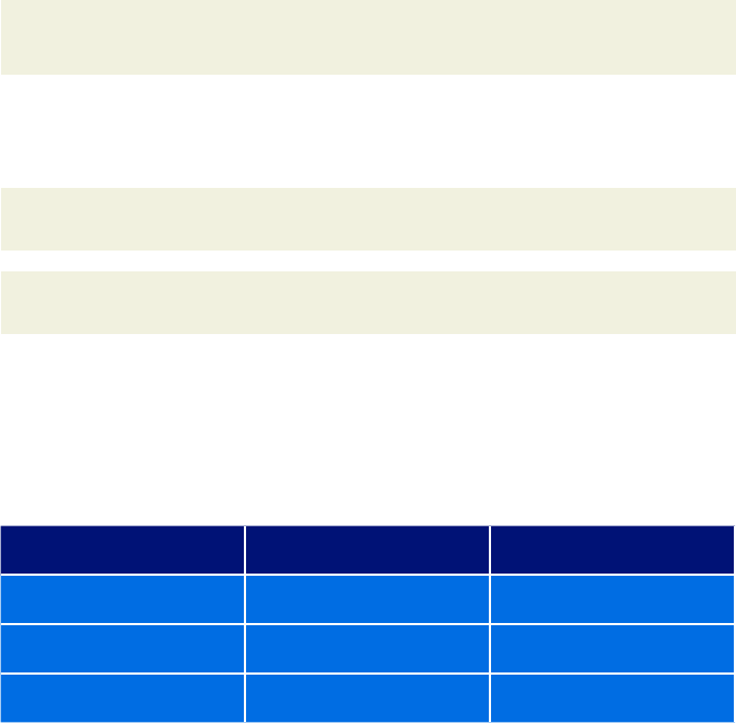
The approach includes three key rating factors
and metrics:
Factor Metric Rationale
Scale Revenue Scale allows for analysis of company’s ability to withstand negative impacts arising from
climate change, as a result of greater nancial resources. Their greater size is often correlated
with increased diversication, both geographically and sectorally, which provides a bulwark
against negative climate risk impacts.
Protability Revenue/Gross
Prot
Companies with greater protability are better positioned to absorb the increased costs that
climate change risks can cause; those companies with low protability may nd the impact of
climate change can push them into a negative nancial position very quickly. In addition, in
analysing intra-sector, companies with greater protability in competitive industries will
likely outcompete others, allowing for analysis of winners and losers from climate change.
Leverage EBITDA/Net Debt Leverage allows for an analysis of the company’s ongoing viability as it relates to:
1 The ability of the company to support its existing long term debt, as climate change risks
impact nancial performance
2 The ability of the company to fund increased investments to transition to a low-carbon
economy
These factors are readily available outputs from
the nancial impact assessment. Additional
non-quantitative factors, such as the company’s
business model and nancial policies were
considered, however it was deemed that such
considerations would be captured when the
outputs of the assessment are reviewed by
subject matter experts, and where these factors
would materially change the outcome, they
would be incorporated at that stage.
The mapping of nancial metrics to credit
ratings for each factor is calibrated based upon
the observable population as of today, including
existing company’s nancial ratios and the
associated company credit rating. This allows for
a scale to be established, for each factor within
each sector, which in turn provides the
foundation for future assessments as
company’s nancial metrics change.
These rating factors are then weighted to
produce a nal credit output, and the weighting
assigned to each is sector dependent. This
reects the fact that certain sectors exhibit
greater reliance on one factor or another when
determining credit rating. The calibration of
these weights has considered both current
importance of the factor in a sector credit
assessment, but also likely future assessments
of credit. This reects the fact that for many
sectors, carbon price costs are not a material
consideration at this time, and so factors such
as Scale (total revenues) may currently play an
outsized role in determining credit strength.
However, in the future it is likely that companies
less exposed to carbon pricing, through lower
emissions, will be better positioned, and
therefore erode the outsized inuence of the
Scale factor. An example of this would be in the
Power Utilities sector,
where currently the scale of a company is one
ofthe most material factors. However, under
scenarios which include signicant carbon taxes,
such scale, if accompanied by associated large
emissions, may work in the opposite direction
and cause rating deterioration as carbon costs
increase. Whilst such changing dynamics may be
challenging to forecast, it is important that
assessments are made sensitive to how credit
rating methodologies may evolve as climate
risks materialize.
Barclays PLC
home.barclays/annualreport 19
Barclays PLC Corporate Transition Risk Forecast Model 2021
The calculation of credit rating, using Barclays DG scale, is as below, where α is the weight on each
factor, for a given sector.
Modeled_DG_t = DG_(levg,t) × α_levg + DG_(prot,t) × α_prot
+ DG_(scale,t) × α_scale ΔModeledDG_t
(24)
This is calculated for all periods in the forecast, as well as the jump-o point. The model then
calculates the delta from the prior period in the modeled DG score, applies the delta to the actual
jump-o DG score from Barclays existing credit systems.
ΔModeledDG_t = ModeledDG_t − ModeledDG_(t−1)
(25)
DG
t
= DG
t-1
+ ΔModeledDG
t
(26)
The approach taken here is in line with the
methodologies aim to capture directionality and
magnitude of impact over a long term time
horizon rather than a very specic degree of
accuracy. There are limitations to such an
approach, including that the DG produced by the
model methodology may dier to the actual DG
on a spot basis, driven principally as outlined
above by the variety of factors the scorecard
does not account for currently.
The below example shows the ratings progression for Company A and B in Example 2 in section 3.1.
For the Oil & Gas sector, the weightings for the scorecard components are as follows:
Factor Metric Weight
Scale Revenue 36%
Protability Revenue/Gross Prot 18%
Leverage EBITDA/Net Debt 46%
3 Financial and Credit Risk Outputs continued
Barclays PLC
home.barclays/annualreport20
Barclays PLC Corporate Transition Risk Forecast Model 2021

Example 2 continued: Company A
In this example, Company A makes the strategic decision to shift away from fossil fuels and towards renewable power as its main source of revenue
generation. The initial increase in Oil Prices at the start of the scenario leads to improved nancial metrics and an improvement in credit grading. As
the scenario progresses and the company transitions to renewables, these new streams of revenue replace fossil fuels bases revenues driving
improvements in the Scale metric. The Leverage metric deteriorates in the middle of the scenario as the rm enacts its transition plans, causing
increased capital expenditure and resulting increase in net debt.
Protability Scale (£mn)
40%
30%
20%
10%
0%
2020 2030 2040 2045 20502025 2035
50,000
40,000
30,000
20,000
10,000
0
2020 2030 2040 2045 20502025 2035
Leverage DG
2.00
1.50
1.00
0.50
0.00
2020 2030 2040 2045 20502025 2035
22
20
18
16
14
12
10
8
6
4
2
0
2020 2030 2040 2045 20502025 2035
Example 2 continued: Company B
In this example, Company B does not transition into renewable power generation, and focuses instead on competing in the fossil fuel space. Whilst
the initial increase in Oil Prices causes improvements in the nancial metrics, resulting in an improved credit rating, the rapid increase in carbon
prices and the falling demand for fossil fuels causes signicant declines in the Scale and Protability metric, whilst Leverage increases before
turning negative as earnings fall below zero. These factors drive a declining credit rating, leading to the company defaulting in 2040.
Protability Scale (£mn)
40%
30%
20%
10%
0%
2020 2030 2040 2045 20502025 2035
25,000
20,000
15,000
10,000
5,000
0
2020 2030 2040 2045 20502025 2035
Leverage DG
6.00
3.00
0.00
-3.00
-6.00
-9.00
2020 2030 2040 2045 20502025 2035
22
20
18
16
14
12
10
8
6
4
2
0
2020 2030 2040 2045 20502025 2035
Barclays PLC
home.barclays/annualreport 21
Barclays PLC Corporate Transition Risk Forecast Model 2021
4 Known Enhancements
The approach is intentionally simplistic,
recognizing that modelling the nancial
performance of companies over a long term
time horizon is inherently fraught with issues and
methodological challenges. Focus has been on
achieving directionality and magnitude of impact
rather than accuracy. To that end, a number of
assumptions are designed to identify potential
winners and losers, rather than the specic
credit rating of a company. There are however a
number of areas of known enhancements to
consider in the future to improve the
performance of the methodology and better
identify and quantify risks.
4.1 Data
The most signicant limitations with the
methodology stem from the lack of consistently
available input data. This is an issue spanning
multiple data types and sources, but is most
acute in terms of nancial data and emissions.
4.1.1 Financial Data
The methodology follows a consistent approach
across a wide breadth of sectors and large depth
of the company types within those, and
therefore it seeks to use consistent data types
and formats, which may not be available for all
companies. For example, within Oil and Gas, cost
of sales data is a less relevant metric for certain
value chain participants (eg. Upstream) and
therefore it is challenging to obtain a meaningful
metric or estimation to integrate into the
methodology. Alternatively, in the case of
smaller private companies, the suite of nancial
metrics produced may not include those
required to perform modelling.
Attributing revenues to specic technology
types presents issues given that this data is
rarely disclosed in the format required. Various
estimation techniques are utilized to derive this
information however there are limitations to
these approaches. For example, in the Power
Utilities sector, the type of generation fuel (eg.
coal vs renewables) is not directly linked to the
generation of revenues, and therefore it is less
clear the direct impact a reduction in demand of
one technology type will have to revenue.
Finally, given the methodology uses jump-o
values to forecast future impacts from climate
scenarios, it is change to: sensitive to the
magnitude of these starting values, that are
unrepresentative of the long run nancial
performance of the company eg. the impact of
COVID-19. When considering a long term time
horizon, a representative starting position for
the company is required from which the impacts
of climate change can be isolated. Using running
averages as a starting point may enhance the
representativeness of the jump-o, to ensuring
it is a fair reection of the company prior to
climate scenarios being applied.
4.1.2 Emissions Data
In order to calculate the impact of carbon prices
to companies, accurate GHG emissions data is
required. Carbon taxes represent one of the
most material drivers of transition risk and
therefore accuracy of emissions is important.
Certain sectors however, and in many cases
smaller companies, are less prone to disclose
their emissions data. In such instances, the
methodology estimates emissions using sector
level nancial intensities. This approach may lead
to discrepancies between emissions utilized by
the methodology and those emitted in reality,
leading to punitive or favorable carbon taxes and
nancial impacts that may be less accurate.
4.2 Modelling Production Vs Revenue
The segmentation and attribution of company
revenues to technologies, and the subsequent
modelling of those revenues over time
depending on changes in relevant scenario
variables, can cause modelling issues. In
particular, there are challenges when considering
the interaction between changing market
dynamics through scenario variables and
company specic actions through adaptation
plans. Calculations of future nancial
performance where the number of assessment
dimensions increase (i.e. starting nancial
performance, scenario variables and company
business operations) becomes challenging as
there are feedback loops and interactions
between them that are not easily isolated.
Future enhancements may consider moving the
modelling approach to focus on production
metrics rather than revenue generation, to
assess revenues sequentially rather than as a
sensitivity. Further work is required to
understand the conceptual requirements for
such an approach, as well as the availability of
data that would support this form of modelling.
4.3 Incorporating Dierent Margins
The approach currently considers prot margins
to be static. Costs are modeled as changing in
line with revenues, which in turn causes margins
to stay the same. The one exception to this is for
Oil & Gas companies where the approach allows
an improvement in margins once the transition
begins, reecting past experience where such
companies implement cost savings to improve
margins in adverse economic climates. In the
future, dynamic margins may be considered and
at a lower level of granularity i.e. sector,
sub-sector or company specic.
Barclays PLC
home.barclays/annualreport22
Barclays PLC Corporate Transition Risk Forecast Model 2021
4.4 Adaptation Sensitivity
Over a long term time horizon, the actions taken
by a company can materially impact the
outcome of the assessment. The adaptation
assessment only considers current plans and
treats them as either credible or not credible
using the credibility criteria outlined. This binary
decision however ignores that in many cases,
companies will endeavor to meet their
commitments, and even in instances where they
do not achieve the desired goal, they will have
made positive steps to either reduce emissions
or transition to low carbon products or services.
These improvements would not currently be
factored into the methodology and may cause
more severe impact assessments than would
likely occur. Possible enhancements to this
include consideration of adaptation on a sliding
scale, where plans may be considered fully
credible and factored in, plans may be
considered not credible (in cases where there
are aspirational statements only and no
supportive evidence) or partially credible, where
the plan is discounted in some manner to
consider that part of the plan is achieved but not
the full commitment. Further enhancements for
consideration include how to factor in that
companies may change business plans over
time further than current commitments as
economies transition and risks and
opportunities from climate change materialize.
4.5 Credit Output
The conversion from nancial impact to credit
impact utilises a simplistic scorecard across
three factors. This is representative of the
inherent challenge of calculating credit impacts
over such a long term time horizon. The current
factors are quantitative in nature, using nancial
metrics which are produced from the
methodology. Additional qualitative factors may
be considered in a review process after the run,
but are not currently factored into the scorecard
calculation and such factors can be signicant in
a number of sectors. One example would be the
level of Regulatory support and cost recovery
ability for Regulated Power Utilities. In addition,
the contribution of factors to the overall credit
score are weighted at a sector level using SME
judgment. These weights are subjective and
may not be appropriately calibrated to represent
the sectors key credit considerations. Finally,
thecredit rating outputs may be reviewed to
consider simplifying the range of outcomes,
away from specic credit ratings and to credit
rating buckets i.e. Investment Grade vs
Non-Investment Grade. Non-Investment
Gradeand sub-categories of these.
4.6 Geographical Granularity of Data
The methodology currently uses scenario
variables and their impact to companies at a
global level and does not dierentiate between
country level dynamics i.e. demand for certain
goods and services may dier from one country
to the next. This is also true of carbon price
where a global carbon price is assumed rather
than one set at a country or regional level. The
necessary company level data required to apply
geographical granularity to the assessment is
currently too onerous and in many cases not
available to support modelling.
4.7 Demand Sensitivity
Changes in scenario demand for products and
services is currently treated as uniform across all
companies with operations in that technology.
For example, a 20% fall in demand for cement
would impact revenues for all cement
companies to the same magnitude. However, a
fall in demand for products and services is likely
to impact dierent companies to dierent
extents, with some more sensitive to a fall whilst
others will remain insulated. This may be a
function of the operational eciency of a
company, slight dierentiation in product
oering or geographical considerations,
amongst others. Enhancements may consider
how to incorporate this sensitivity to demand
into the model, and to this end initial
assessments have been undertaken for
companies in the Oil & Gas sector, where certain
factors of a company (eg. size) be considered as
an indicator of how scenario demand would
translate to company demand.
4.8 Stranded Assets
The methodology currently focuses on changes
in revenues and costs i.e. income statement
metrics, rather than on balance sheet items
such as assets. Changes in the demand for fossil
fuels, and the reduction under transition risk
scenarios, may cause the value of company
assets to change and in some cases fall eg.
stranded oil reserves for oil & gas clients. These
changes in assets may in turn cause companies
to suer nancial deterioration which would
drive higher credit risk, which the approach does
not currently factor in.
Barclays PLC
home.barclays/annualreport 23
Barclays PLC Corporate Transition Risk Forecast Model 2021

Registered oce: 1 Churchill Place, London E14 5HP
© Barclays PLC 2022
Registered in England. Registered No: 48839
