

Lesson: May 4, 2020
Objective/Learning Target:
Students will learn how to format cells to help personalize
their files

Introduction
After you've added a lot of content to a spreadsheet, it can sometimes be difficult to view and read all
of your information easily. Formatting allows you to customize the look and feel of your spreadsheet,
making it easier to view and understand.
In this lesson, you'll learn how to modify the size, style, and color of text in your cells. You will also
learn how to set text alignment and add borders and background colors to your cells.

Formatting Cells
Every cell in a new spreadsheet uses the same default formatting. As you begin to build a
spreadsheet, you can customize the formatting to make your information easier to view and
understand. In our example, we will be using a spreadsheet to plan and organize a garden plot.

Change the Font Size
Excel
The AutoFit feature will allow you to set a column's width to fit its
content automatically.
1. Select the cell(s) you want to modify.
2. On the Home tab, click the drop-down arrow next to the
Font Size command, then select the desired font size. In
our example, we will choose 24 to make the text larger.
3. The text will change to the selected font size.
Google Sheets
Modifying the font size can help call attention to important cells and
make them easier to read. In our example, we will be increasing the
size of our header cells to help distinguish them from the rest of the
spreadsheet.
1. Select the cell or cells you want to modify.
2. Locate and select the Font Size button in the toolbar, then
choose the desired font size from the drop-down menu. In our
example, we will choose 14 to make the text larger.
3. The text will change to the new font size.

Excel
By default, the font of each new workbook is set to Calibri.
However, Excel provides many other fonts you can use to
customize your cell text. In the example below, we'll format our
title cell to help distinguish it from the rest of the worksheet.
1. Select the cell(s) you want to modify.
2. On the Home tab, click the drop-down arrow next to the
Font command, then select the desired font. In our
example, we'll choose Century Gothic.
3. The text will change to the selected font.
Sheets
1. Select the cell or cells you want to modify.
2. Locate and select Format in the toolbar menu.
3. Hover the mouse over Font, then select a new font
from the drop-down menu. In our example, we'll select
Georgia.
4. The text will change to the new font.
Change the Font

Excel
1. Select the cell(s) you want to modify.
2. On the Home tab, click the drop-down arrow next to the
Font Color command, then select the desired font color.
In our example, we'll choose Green.
3. The text will change to the selected font color.
Sheets
1. Select the cell or cells you
want to modify.
2. Locate and select the Text
color button in the toolbar.
3. A drop-down menu of
different text colors will
appear.
4. Select the color you want to
use. In our example, we'll
select red
5. The text will change to the new color.
Change the Text Color

Cell Borders and Fill Colors
Cell borders and fill colors allow you to create clear and defined boundaries for different sections of
your worksheet. Below, we'll add cell borders and fill color to our header cells to help distinguish them
from the rest of the worksheet.

Add A Fill Color
Excel
1. Select the cell(s) you want to modify.
2. On the Home tab, click the
drop-down arrow next to the Fill
Color command, then select the fill
color you want to use. In our
example, we'll choose a dark gray.
3. The selected fill color will appear in the selected cells.
We've also changed the font color to white to make it
more readable with this dark fill color.
Sheets
1. Select the cell or cells you want
to modify.
2. Locate and select the Fill color
button from the toolbar.
3. Select a color from the
drop-down menu. In our
example, we'll choose blue.
4. The new fill color will
appear

Add a Border
Excel
1. Select the cell(s) you want to
modify.
2. On the Home tab, click the
drop-down arrow next to the
Borders command, then select
the border style you want to use.
In our example, we'll choose to
display All Borders.
3. The selected border style will
appear.
Sheets
1. Select the cell or cells you want to modify.
2. Select the Borders button and choose the desired border
option from the drop-down menu. In our example, we'll
choose to display all cell borders
3. The new cell borders will appear.

Text Alignment
By default, any text entered into your worksheet will be aligned to the bottom-left of a cell, while any numbers will be aligned to the
bottom-right. Changing the alignment of your cell content allows you to choose how the content is displayed in any cell, which can make
your cell content easier to read.

Change Horizontal Text Alignment
Excel
1. Select the cell(s) you want to
modify.
2. Select one of the three
horizontal alignment
commands on the Home tab. In
our example, we'll choose
Center Align.
3. The text will realign.
Sheets
1. Select the text you want to
modify.
2. Click the Horizontal align
button in the toolbar, then
select the desired alignment
from the drop-down menu.
3. The text will realign.
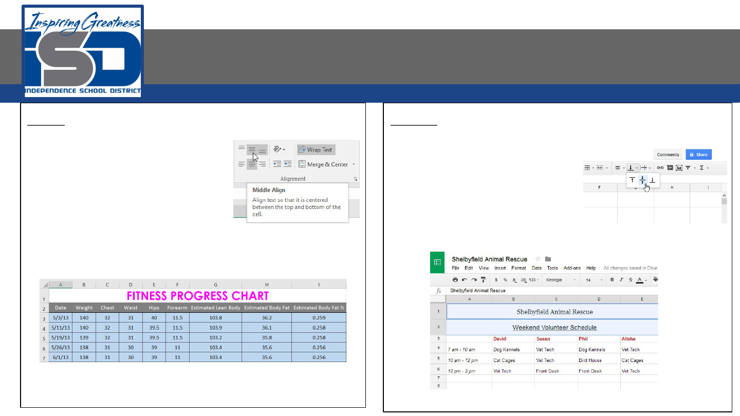
Change the Vertical Alignment
Excel
1. Select the cell(s) you want to
modify.
2. Select one of the three vertical
alignment commands on the
Home tab. In our example,
we'll choose Middle Align.
3. The text will realign.
Sheets
1. Select the text you want to modify.
2. Click the Vertical align button in
the toolbar, then choose the
desired alignment from the
drop-down menu.
3. The text will realign.

Challenge
Excel
1. Open Excel 2016.
2. Type Challenge in cell A1
3. Merge and Center Cells A1:A6
4. Select cells A1:E6. Change the horizontal alignment to
center and the vertical alignment to middle.
5. Select cell A1. Bold the text and add an outside border.
6. Select the merged cell in row 1 and change the font to
something other than Arial.
7. With the cell still selected, change the font size to 18 pt and
bold the text.
8. For the same cell, change the fill color to purple and the
font color to white.
Sheets
1. Open Google Sheets and create a new blank spreadsheet.
2. Type Challenge in cell A1
3. Merge and Center Cells A1:A6
4. Select cells A1:E6. Change the horizontal alignment to
center and the vertical alignment to middle.
5. Select cell A1. Bold the text and add an outside border.
6. Select the merged cell in row 1 and change the font to
something other than Arial.
7. With the cell still selected, change the font size to 18 pt and
bold the text.
8. For the same cell, change the fill color to purple and the
font color to white.

