NBER WORKING PAPER SERIES
WHAT DOES MONETARY POLICY DO TO LONG-TERM INTEREST RATES
AT THE ZERO LOWER BOUND?
Jonathan H. Wright
Working Paper 17154
http://www.nber.org/papers/w17154
NATIONAL BUREAU OF ECONOMIC RESEARCH
1050 Massachusetts Avenue
Cambridge, MA 02138
June 2011
I am grateful to Tobias Adrian, Joseph Gagnon, Refet Gürkaynak and Eric Swanson for helpful discussions.
All errors are my sole responsibility. The views expressed herein are those of the author and do not
necessarily reflect the views of the National Bureau of Economic Research.
NBER working papers are circulated for discussion and comment purposes. They have not been peer-
reviewed or been subject to the review by the NBER Board of Directors that accompanies official
NBER publications.
© 2011 by Jonathan H. Wright. All rights reserved. Short sections of text, not to exceed two paragraphs,
may be quoted without explicit permission provided that full credit, including © notice, is given to
the source.

What does Monetary Policy do to Long-Term Interest Rates at the Zero Lower Bound?
Jonathan H. Wright
NBER Working Paper No. 17154
June 2011
JEL No. C22,E43,E58
ABSTRACT
The federal funds rate has been stuck at the zero bound for over two years and the Fed has turned to
unconventional monetary policies, such as large scale asset purchases to provide stimulus to the economy.
This paper uses a structural VAR with daily data to identify the effects of monetary policy shocks
on various longer-term interest rates during this period. The VAR is identified using the assumption
that monetary policy shocks are heteroskedastic: monetary policy shocks have especially high variance
on days of FOMC meetings and certain speeches, while there is nothing unusual about these days from
the perspective of any other shocks to the economy. A complementary high-frequency event-study
approach is also used. I find that stimulative monetary policy shocks lower Treasury and corporate
bond yields, but the effects die off fairly fast, with an estimated half-life of about two months.
Jonathan H. Wright
Department of Economics
Johns Hopkins University
3400 N. Charles Street
Baltimore, MD 21218
and NBER
1 Introduction
During the recent financial crisis, the Feder al Reserve sharply lowered the targ et for
the federal funds rate. In D ecember 2008, the federal fund s rate was set to the zero
lo wer bound (mo re precisely in a target range from zero to 25 basis poin ts), and
has remained there since then. With monetary policy stuc k at the zero bound, the
Federal Open Market C o m m ittee (FOMC) began using other, less conven tiona l, w ays
to further stim ulate aggregate demand. This included statements signaling that the
funds rate would be k ept at the zero bound for a long time, programs geared to wards
supporting certain critical credit markets that were frozen, suc h as the Commer cial
Paper Funding Facility and the Term Asset-Back ed Securities Loan Facility. And it
included p roviding add itional stimulus to the economy by large-scale asset purchases
(LSAPs) of Treasury securities and other high-grade bonds, a policy that is commonly
referred to as quantitative easing. A k ey motivation for these purchases w as to try
to lo wer the in terest rates being paid by households and businesses, so as to support
consumption and in v estment spending. The rationale put forth b y Federal Reserve
officials mainly relies on a preferred habitat paradigm , as envisio ned by Modigliani
and Sutc h (1966, 1967) and more recently by Vayanos and Vila (2009) in which
markets are segmen ted, in vestors demand bonds of a specific type, and the interest
rate is determined by the supply and demand of bonds of that particular t ype (Kohn
(2009)). The LSAP s could also w o rk in other ways, such as by affecting agen ts’
expectations of the future course of monetary policy.
More than two years after the o vernight rate hit the zero bound, there is a rapidly-
growing literature on assessing the effects of the unconv entional monetary policies
that ha ve been used o ver this period. Important contributions include Doh (2010),
D’Amico and King (2010), Gagnon et al. (2010), Hamilton and Wu (2010), Neely
1
(2010), H ancock and P assm ore (2011) and Krishnamurth y and Vissing-Jorgenson
(2011). Also, Swanson (2011) reexamined Operation Twist from the 1960s using an
event-stud y perspectiv e, and compared it to the unco nventional mo netary policies
presently being emplo yed b y the Federal Reserve.
Measuring the effects of monetary policy shoc ks in this environment ho wev er poses
special challenges. In normal times, the federal funds rate measu res the stance of
monetary policy. But things are m urkier at the zero bound. There isn’t as clean a
single measure of the o verall stance of unconventional monetary policy. And while one
could proxy the stance of monetary policy by the size of the Fed’s balance sheet, with
forward-looking fina ncial markets, one w o uld expect a policy of asset purchases to
impact asset prices not at the time that the purchases are actually made, but rather
at the time that in vestors learn that they will take place. LSAPs are anno unced ah ead
of tim e, in th e statemen ts that follow FOM C meetings. These statements are in turn
anticipated to some exten t b y in vestors, whose expectations ha ve been guided by
speec hes and other comments b y FO M C members. Furthermore, whereas the federal
funds futures market giv es a fairly clear measure of investors’ real-time expectations
for c h ang es in the target federal funds rate, there is no such measure of expectations
ofthesizeofLSAPs.
In this paper, I propose measuring the effects of moneta ry policy shock s during
this period of uncon ven tion al m o netary policy using a stru ctu ral vector autoregression
(VAR ) in financial variables at the daily frequency, employing the methodology of
Rigobon (2003) and Rigobon and Sack (2003, 2004, 2005). The idea is to iden tify
days on which the variance of mo neta ry policy shoc ks was especially h igh, during the
period when the federal funds rate was stuck at the zero bound and unconv entional
approac hes monetary policy were being deployed. These are da ys of FOMC meetings
and da ys with other announcements that apparen tly altered inv estors’ views about the
2
lik ely extent of mon etary policy actions. Com paring the variance-covariance matrix
of VAR inno vations on these and other days enables iden tification of the effects of
these monetary policy shocks. In principle, this goes back to the idea of measuring
mon etary policy shock s in a VAR of Sims (1980), Bernanke (1986) and Christiano,
Eichenbaum and Evans (1996), but it does so without t ying monetary policy decisions
to the level of the target federal funds rates. But unlike the earlier VAR literature,
identification does not depend on the standard short-run zero restrictions. Instead,
this is an identification strategy using heterosk ed asticity in daily-frequency data.
It should be emphasized that this approach addresses a somewha t different ques-
tion from the analysis of the effects of LSAPs by Gagnon et al. (2010), Krishn amurthy
and Vissing-Jorgenson (2011) and other authors. My approach here identifies policy
shocks from the total effect of FOMC -related news on a set of asset prices during
this period of unconventional monetary policy. FOMC statements could impact asset
prices via LSAPs–LSAPs are surely the dominant tool of monetary policy when the
economy is stuc k at the zero bound. But FO M C statemen ts could also work in other
w ays, such as by signaling that the federal funds rate will be kept lo w (ov er and above
the signa ling effect of LSAPs), or even by c hanging agents’ beliefs about the under-
lying state of the economy (if they think that the Fed has some private information ).
The proposed methodology measures the total effects of FOMC new s and cannot dis-
en tan gle the effects of these different chan nels. Of course, the separate iden tification
of the effects of different F O MC statements is an important question. Noneth eless,
the structural VAR approach considered here brings some importan t advan tages. It
circumvents the difficulties in measuring market expectations for Fed statements–it
isn’t necessary to specify what the mar kets learned from Fed statements, it is only
necessary to specify the times at which a significant news came out, a much easier
task. It allows for the possibilit y that other shock s occurred on the same days as
3
the monetary policy shocks. And it pro vides an estimate of the persistence of the
mon etary policy shocks, which the standard event-stud y methodology cannot do.
Over the period since Nov ember 2008, I estimate that monetar y policy shocks
ha v e a significant effect on ten-year yields and long-maturity corporate bond yields
that wear off o ver the next few months. The effect on tw o-year Treasu ry yields is ve ry
small. The initial effect on corporate bond yields is a bit more than half as large as
the effect on ten-year Treasury yields. This finding is importan t as it sho w s that the
news about purchases of Treasury securities had effects that w er e not limited to the
Treasury yield curve. That is, the monetary policy shocks not only impacted Treasury
rates, but were also transmitted to private yields which have a more direct bearing
on economic activity. There is slight evidence of a rotation in break even rates from
Treasury Inflation Protected Securities (TIPS), with short-term break evens rising and
long-term forward breakev ens falling.
The plan for the remainder of this paper is as follows. Section 2 discusses the
meth odology and the identifying assumptions. Section 3 describes the data and re-
ports the results of the empirical w ork. Section 4 discusses a closely-related “event-
study” approac h that relates the VAR errors to monetary policy surprises measured
using high-frequency intradaily data in small windo ws that brac ket the announce-
ment times. This alternative methodology ends up giving consistent results, but with
estimates that are somew ha t more precise. Section 5 concludes.
2TheMethod
I assume that a x1 v e ctor of yields,
, has the reduced form VAR representation
()
= +
(1)
4
where
denote the reduced form forecast errors. I further assume that these reduced
form errors can be related to a set of underlying structural shocks
= Σ
=1
(2)
where
is the th structural shock,
is a x1 v ector, and the structural shoc ks
are independent of eac h other and o ver time. The parameters (), and {
}
=1
are all assumed to be constan t.
The monetary policy shock is ordered first but this is for notational convenience
only. The ordering of variables is irrelevant as a Choleski decomposition will not be
used for identification. The monetary policy shock has mean zero and variance
2
1
on announ cem ent da y s, and variance
2
0
on all other days, while all other structural
shocks are identically distributed with mean zero and variance 1 on all dates. The
identifying assumpt ion is that
2
0
6=
2
1
. Put another w ay, the identifying assumption
is that news about monetary policy comes out in a lump y manner, and the days on
which it comes out are determined b y acciden t of the calendar; and so the volatility
of other structural shocks should be identical on these and other days. This strategy
of iden tification through heteroskedasticit y was first proposed b y Rigobon (2003) and
applied to asset price data b y Rigobon and Sack (2003, 2004, 2005), becoming quite
popular in the iden tification of structural VARs since then.
Let Σ
0
and Σ
1
denote the variance-covariance matrices of reduced form errors on
non-announcement and announcement days, respectiv ely. Clearly,
Σ
1
− Σ
0
=
1
0
1
2
1
−
1
0
1
2
0
=
1
0
1
(
2
1
−
2
0
) (3)
Th is allows
1
to be identified. Without loss of generalit y, I adopt the normalization
5
that
2
1
−
2
0
=1,as
1
0
1
and (
2
1
−
2
0
) are not separately identified. I am seeking only
to identify the effects of monetary policy shocks, not the other structural shocks in
the VAR (
2
), therefore imposing further structure on the system is not needed.
The econ om etric stra tegy is to estimate the VAR and construct the sample variance-
co variance matrices of residuals on non-annou ncem ent and announcem ent da y s, re-
spectiv e ly,
ˆ
Σ
0
and
ˆ
Σ
1
. Then the parameters in the vector
1
can be estimated b y
solving the minimum distance problem
ˆ
1
=argmin
1
[(
ˆ
Σ
1
−
ˆ
Σ
0
) − (
1
0
1
)]
0
[
ˆ
0
+
ˆ
1
]
−1
[(
ˆ
Σ
1
−
ˆ
Σ
0
) − (
1
0
1
)]
(4)
where
ˆ
0
and
ˆ
1
are estimates of the variance-covariance matrices of (
ˆ
Σ
0
) and
(
ˆ
Σ
1
), respectively. Estim a tes of the impulse responses can then be traced out.
This leaves the question of statistical inference. Use of the bootstrap may help
to mitigate concerns about statistical inference in a small sample size. I do bootstrap
inference in three parts. First, I want to test the hypothesis that announcemen t
and non-announcement days are no different: that Σ
0
= Σ
1
. I do this using the test
statistic
[(
ˆ
Σ
1
−
ˆ
Σ
0
)]
0
[
ˆ
0
+
ˆ
1
]
−1
[(
ˆ
Σ
1
−
ˆ
Σ
0
)] (5)
and comparing it to a distribution in which announcement and non-announcement
days are randomly scrambled, so that the two variance-covariance matrices are equal
b y construction under the null in the bootstrap samples. Rejection of this null hy-
pothesis mean s that the identifica tio n condition is satisfied.
Second, I w an t to conduct inference on the structural impulse responses, given that
they are iden tified. As the data are persistent, I use the bias-adjusted bootstrap of
Kilian (1998), except that instead of resampling from individual v ectors of residuals,
6

I use the stationary bootstrap (Politis and Romano (1994)) to resample blocks of
residuals of expected length of 10 days. This means that the bootstrap should preserve
some of the volatility clustering that is evident in the original data.
1
This allows
confidence intervals for the impulse responses to be constructed. This bias adjustment
is also applied to the poin t estimates.
Finally, this same bootstrap can be used to test the hypothesis that Σ
1
− Σ
0
=
1
0
1
, in other words that there is a single monetar y policy shoc k. This is done b y
comp aring the test statistic
[(
ˆ
Σ
1
−
ˆ
Σ
0
) − (
ˆ
1
ˆ
0
1
)]
0
[
ˆ
0
+
ˆ
1
]
−1
[(
ˆ
Σ
1
−
ˆ
Σ
0
) − (
ˆ
1
ˆ
0
1
)] (6)
to the distribution from the bias-adjusted bootstrap.
2
3DataandResults
In the baseline imp lem e ntation of this method, I use daily data on six different interest
rates from the period No vem ber 3 2008 to December 28 2010. These are the two- and
ten-year nominal Treasury zero-coupon yields from the data set of Gürka ynak, Sack
and Wrigh t (2007), the five-yea r TIPS breakev en
3
and the five-to-ten-y ear forw ard
TIPS break even, from the data set of Gürkaynak, Sac k and Wright (2010) and the
Moody’s indices of BAA and AAA corporate bond yields (not spreads). A VAR (1)
was fitted to these data.
Table 1 shows the list of 21 monetary policy announcement da ys. The criterion
1
Simply resampling from the residuals in the usual way would ho wever give very similar results.
2
More precisely, if
ˆ
Σ
∗
0
,
ˆ
Σ
∗
1
,
ˆ
∗
1
,
ˆ
∗
0
and
ˆ
∗
1
denote the bootstrap analogs of
ˆ
Σ
0
,
ˆ
Σ
1
,
ˆ
1
,
ˆ
0
and
ˆ
1
, respectively, then the bootstrap simulates the distributions of
0
[
ˆ
∗
0
+
ˆ
∗
1
]
−1
where =
(
ˆ
Σ
∗
1
−
ˆ
Σ
∗
0
) − (
ˆ
∗
1
ˆ
∗0
1
) − ((
ˆ
Σ
1
−
ˆ
Σ
0
) − (
ˆ
1
ˆ
0
1
)).
3
This is the spread between a nominal and TIPS bond, also known as inflation compensation. It
is influenced by expected inflation, the inflation risk premium, and the TIPS liquidity premium.
7

for inclusion in this list is that it be either the day of any F O M C meeting during the
period in whic h monetary policy was stuck at the zero bound,
4
or the day of another
announcem ent or speec h by Chairman Bernank e that was seen as especially germane
to the prospects for LSAPs. One might of course include days of other speec hes or
releases of FO MC minutes. I did not do so, because it is importan t that the esti-
mation of the variance-covariance matrix on announcem ent da y s is not con ta m inated
with da ys on which there is only trivial or indirect news about unconv entional mon e-
tary policy; that will only blunt the distinction between the two variance -covariance
matrice s that is crucial to iden tification.
ThedayslistedinTable1spanboththefirst period of quantitative easing (QE 1),
during whic h time the Fed bought a range of assets including a large volume of
mortg age backed securities and the second period of quantitativ e easing (QE2), wh ich
in volved Treasury purc h ases alone. Within the 21 da ys listed in Table 1, 10 of them
are day s that seem especially important–they are da y s around the start of the first
and second phases of quantitativ e easing. These especially important annou nc em e nt
days are mark ed in bold.
The variance-covariance matrix of reduced form errors was then estimated over
the 21 announcem e nt days, and o ver non-announ cem ent da ys. The m ethod described
in the previous section w as then used to estimate
1
, the contemporaneous effects of
a monetary policy shock on yields.
The resulting impulse responses function estimates and 90 percent bootstrap confi-
dence inte rvals in this baseline VAR are reported in Figure 1. The identified monetary
policy shoc k is normalized to lower ten-year yields by 25 basis points instan taneously.
4
December 16, 2008 was included. This was the day of the FOMC meeting at which the funds
rate was set at zero, but the statement also included discussion of LSAPs. The unscheduled FOMC
meeting of May 9, 2010 (after which a statement related to foreign exchange swaps was released) is
not included because it has no direct bearing on domestic monetary policy.
8

The shock lowers AAA and BAA rates, by a bit more than half as muc h as the drop
in ten-ye ar Treasury yields. These effects tend to wear off over time fairly fast–the
impu lse responses on ten-y ear Treasur ies are statistically significant, but only for a
short time. The effect on corporate yields is statistically signific ant in this VAR, but
only for a very short time. Two-year yields fall, but the effect is modest.
5
The half-life
of the estimated impulse responses for Treasury and corporate yields is one or two
months. Short-term break even rates rise sligh tly, while longer-term forward breakev en
rates fall, but these effects are not statistically significan t. The estimates of the ini-
tial effects are mostly consisten t with the evidence from ev ent studies. For example,
Krishnamurthy and Vissing-Jorgenson (2011) found that quantitative easing policies
lo wer long-term Treasuries and the highest rated corporate bonds, and report some
evidence that break even rates rise. They ho wever found that quan titative easing has
neglig ib le effects on BAA rates.
The top panel of Table 2 reports the results of comparing the test statistics in
equations (5) and (6) with their bootstrap p-values in this baseline VAR. The null
h y pothesis that the reduced form variance-co variance matrix is the same on announce-
men t and non-announcement da ys is rejected. The null h ypothesis that the difference
bet ween the two variance-covariance matrices can be factored in the form
1
0
1
is not
rejected. That indicates that the data can be w ell characterized by a single monetary
policy shock.
The structural VAR approac h measures the monetary policy shock directly from
its effects on interest rates. As noted in the introduction, this has a n umber of advan-
tages: expectations do not ha ve to be measured, and dynamic effects can be traced
5
Ob viously over this period, monetary policy shock s could have no effect on the federal funds
rate or other very short-term interest rates by construction. But the two-year yield was not at the
zero bound (it averaged 81 basis points over the sample), and so monetary policy surprises could
conceivably have had some effectonthis. However,itturnsoutthattheeffect is small.
9
out. Ho wever, it also has a n u mber of limitations. In particular , it is silent on the
relativ e contribution of different aspects of uncon ven tional monetary policy (forward
looking guidance about the federal funds rate, LSAPs etc.). Nev erth eless, looking at
the evidence here in conjunction with other studies that have considered the effects of
asset purchases more directly, and also noting that the main effect of monetary policy
shocks during the crisis is on long-term interest rates, while short-term interest rates
are little changed, it seems reasonable to surmise that LSAPs represent an important
component of these iden tified policy shocks.
3.1 Robustness c hec ks and extensions
This subsection reports the results of three t y pes of extensions and robustness checks.
First,theanalysisisredoneusingthemorestringentdefinition of the announcement
dates (only the announcemen t days marked in bold in Table 1). This should make the
difference between policy and non-policy dates starker, potentially helping identifica-
tion. Impulse response estimates are show n in Figure 2. The results are quite similar
to those in Figure 1, except that the impu lse responses are a little more precisely
estimated in this case, and the decline in longer-term corporate yields is statistically
significant for a month or so.
The second robustness chec k is for the sample period ch osen to estimate the VAR.
The baseline VAR is estimated over a short sample period. A natural alternative is
to consider estimating the reduced form parameters in () over the period since
Jan u ar y 1999 (when the TIPS yields are first available), while continu in g to estimate
Σ
0
and Σ
1
on non-announcem ent and announcem ent da ys starting in No vem ber 2008.
This gives the poten t ial benefitofgreaterefficiency, although at the potential cost of
ha ving to impose the same coefficients of the VAR in the crisis and pre-crisis periods.
10

The results of this exercise are sho w n in Figure 3. They are aga in qualitativ ely similar
to those show n in Figure 1. However, the effects on ten-y ea r Treasury yields remain
significant for about three months, and the effects on long-term corporate yields are
also significant for a while.
I also consider an alternativ e specification for the set of variables included in the
VAR, replacing the corporate bond yields withtheyieldoncurrent-couponthirty-
y e ar Fannie Mae mortgage backed securities.
6
The results of this exercise are show n
in Figure 4. The monetary policy shock that lowers ten-y ear Treasury yields b y 25
basis points is estimated to lo wer MBS rates b y about 15 basis poin ts. The effect is
statistically significant for a month or so, but the effect again wea rs off fairly quickly.
This paper does not differentiate between the first and second phases of quan titative
easing (QE1 and QE2, respectiv ely). However, QE1 in volv e d heav y purc h ases of
MB S, whereas QE 2 en tailed purchases of Treasuries only. It seems reasonable to
surmise that if one were able separately to iden tify monetar y policy shocks in these
t wo subperiods, then the sensitivity of MBS rates w ou ld be bigger in QE1 than in
QE2.
7
Finally, I also consider an alternative specification for the set of variables included
in the VA R, replacing the corporate bond yields with the sum of the Markit five-year
investment grade corporate CDS index and the five-y ea r swap rate. Under CDS -bond
arbitrage, this should theoretically be close to a fiv e-year in vestment grade corporate
bond yield. The monetary policy shock significantly lowers this syn thetic CDS -based
6
Current coupon securities are benchmark mortgage backed securities (MBS). Naturally one
would be most interested in actual mortgage rates, rather than the yields on MBS, from the perspec-
tive of assessing the ability of monetary policy to support the housing market. However, mortgage
rates are not available at the daily frequency, and so MBS rates are the best available substitute for
use in this paper.
7
In other (not reported) robustness checks, I considered trivariate VARs with two- and ten-year
nominal Treasury yields plus one other int erest rate (a breakeven rate, a corporate bond yield, or the
MBS yield). These VARs again gave similar results, though in some cases the confidence intervals
were a bit tighter.
11
corporate bond yield, but the effect wears off in the subsequent months.
Table 2 includes the specification tests of the h ypotheses that Σ
0
= Σ
1
and that
Σ
1
− Σ
0
canbefactoredintotheform
1
0
1
for the alternative definition of announce-
ment dates, the alternative sample period for estimating (), and the alternativ e
c ho ices of variables in the VAR. In all these cases, the hypothesis that announcem ent
and non-announcem ent da ys are equivalen t is rejected, while the h ypothesis of a single
mon etar y policy shock is accepted.
3.2 Avoiding estim atin g the VAR
An alternative approach is to a void estimating a VAR altogether, and instead simply
assume that the expectation of eac h int erest rate on day is well approxima ted
by it’s value on day − 1. This means that the one-step-ahead forecast errors,
,
cansimplybeapproximatedby∆
.Thedifferen ce between the variance-co variance
matrix of ∆
on announcement and non-announcemen t days can again be factored
as in equation (3), giving estima tes of the instantaneous impulse responses of the
mon etar y policy shock. Ho wever, in avoiding estimating a VAR, this approach giv es up
on trying to estimate the impulse responses at longer horizons. Indeed this approach
of treating the daily first differences as appro xim ate reduced form errors was employed
b y Rigobon and Sack (2005).
The results are show n in Table 3. The size of the monetary policy shoc k is normal-
ized to be one that lowers ten-yea r Treasury yields b y 25 basis poin ts. It generates
causes a small and not quite statistically significan t drop in two-y ear yields, and
significantly lowers corporate bond yields. The instantaneous impulse responses are
qualitatively similar to those from estimating the VAR, although the poin t estimate
of the impact on corporate yields is a bit larger.
12

4 Even t-study methodology and intradaily data
Iden tification through heteroskedasticity collapses to the ev ent-study methodology in
the limiting case that the announcem ent windows contain only the shoc ks that we
wish to identify—that is, when the variances of all other shoc ks are negligible. That’s a
stronger assumption, and is surely not reasonable using daily data, especially over this
turbulen t period, but it migh t be an adequate appro ximation when high-frequen cy
in tra da ily data are used. To consider an event-study methodology, I took quotes on
the front contracts on two-, five-, ten- and thirt y-year bond futures trading on the
Chicago Mercantile Exchange (CME) from Tickdata. Table 1 shows the times of each
of the announcemen ts. The monetary policy shoc k is computed as the first principal
component of yield chan ges
8
from 15 min utes before each of these announcements
to 1 hour and 45 minutes afterwards, re-scaled to have a standard deviation of one,
and signed so that a positive surprise represen ts falling yields.
9
No macroeconomic
news announcem ents occurred in any of these windo w s and so it seems reasonab le to
assume that the monetary policy shoc k w as the overwhelm ing driver of asset prices
in these time periods. Unlike in the event studies of Gagnon et al. (2010) and
Krishn amurthy and Vissing-Jorgenson (2011), the moneta ry policy surprises are being
measur ed directly from intraday cha ng es in asset prices.
The approach here is similar in spirit to that of Gürkaynak, Sack and Sw anson
(2005). These authors recogn ized that FOMC statements con tained both news about
the current setting of the federal funds rate and about its lik ely future trajectory.
8
Yield changes were constructed as returns on the futures con tract divided by the duration of
the cheapest-to-deliver security in the deliverable basket.
9
This is a fairly wide window, but results are similar using a tighter window from 15 minutes before
the announcement to 15 min utes afterwards. However, the announcements considered represent the
in terpretation of statements and speeches, as opposed to giving information about the numerical
value of the target funds rate. Consequently, it seems natural to allow a relatively wide window for
themarkettodigestthenews.
13

Following many other papers (going bac k to Kuttner (2001)), they proposed using
current and next-month federal funds futures quotes to measure the surprise compo-
nent of the setting of the target federal funds rate– th eir key innovation w as that they
proposed using the orthogonal change in four-quarter-ahead eurodollar futures rates
as an asset-price-based quantification of the separate information in the statement
about the outlook for monetary policy going forw ard. They called these the target
and path surprises. Ho wever, since December 2008, there ha ve been no surprises in the
target federal funds rate, and F O M C statements have done little to monetary policy
expectations o ver the next few quarters. Under these circumstances, it seems perhaps
more appropriate to use c han ges in longer-term in terest rates as an asset-price-based
quan tification of monetary policy surprises during this period of unconventional pol-
icy.
10
This directly resolv es the problem faced b y event studies suc h as Gagno n et
al. (2010) and Krishnamurth y and Vissing-Jorgenson (2011) that they did not ha ve
data on market expectations concerning the size of LSAPs.
Table 4 reports the slope coefficien ts from regressions of variou s yield c ha nges
and asset price returns on to the mon etary policy surprises, measured as described
in the previous par agrap h , over the 21 da y s listed in Table 1. The left-hand-side
variables are not limited to the variables considered in the VAR. Note that in these
regressions, whereas the righ t-ha nd -side variable is constructed using high-frequency
in tradaily data; the left-hand side variables are daily chan ges, except for stock index
futures, which are available in tra da ily.
11
A one standard deviation moneta ry policy surprise is estimated to lower ten-y ear
Treasury yields by 14 basis points. For comparison, Gürkaynak, Sack and Sw an son
10
Another option would be to use intradaily changes in longer-term eurodollar futures quotes, but
these are quite illiquid at maturities beyond a year or two, and so the use of Treasury futures is
preferable.
11
These are returns on the S&P futures contract trading on the CME from Tickdata, from 15
min u tes before each announcement to 1 hour and 45 minutes afterwards.
14

(2005) estimated that o ver a period before monetary policy hit the zero bound, it
would tak e a 100 basis poin t surpr ise cut in the target funds rate to lo wer ten-yea r
Treasury yields by about this much. In Table 4, corporate bond yields are estimated
to fall by about 9 basis points (a bit more than half as muc h as the decline in ten-
y e ar Treasury yields), while t wo-year Treasury yields again fall only a little. There is
a rotation of TIPS breakevens, with fiv e-year breakevens rising and fiv e-to-ten-year
forward break evens falling. A possible in ter pretation is that the stronger outlook
for demand boosts the short-to-medium -run inflation outlook, but the fact that the
LSA Ps are overw helm in gly concen trated in nominal (rather than TIPS) securities has
an offsetting effect, pushing longer-term break evens lower. A one standard deviation
mon etary policy surprise is estimated to lower Cana dian, UK and Germa n ten-yea r
go vernment bond yields
12
b y one-third to one-half as much as the decline in ten-year
US Treasury yields—this indicates that the mon etary policy actions have impacted
global expectations for short-term interest rates and/or global risk premia. Rates
on curren t coupon thirty-year Fannie Mae mortg age backed securities fall about 9
basis poin ts. Corporate spreads constructed as the sum of five-year swap rates and
investm e nt grade CDS drop about 15 basis points. Stock prices rise; a monetar y
policy surprise that lowers ten-ye ar yields by 14 basis poin ts is estimated to boost
stoc k returns b y a bit o ver half a percen tage point
13
. All of these effects are highly
statistically significant, even though the left-hand-side variable is measured at the
daily frequency in most cases, and even thoug h the samp le size is just 21 observations.
The SMB factor of Fama and French (returns on small stocks less returns on big
stoc ks) is not significantly affected, consisten t with the finding b y some researchers
12
These are zero-coupon yields obtained at the daily frequency from the websites of the Bank of
Canada, Bank of England and Bundesbank, respectively.
13
For comparison, Bernanke and Kuttner (2005) estimated that, before the zero bound was
reached, an unanticipated 25 basis point surprise reduction of the federal funds rate raised stock
prices by about 1 percent.
15

that in recent decades size does not seem to be a priced risk factor in equity mark e ts
any more
14
. But the monetary policy shock does significantly increase the HM L factor
(returns on value stocks less returns on growth stoc ks). P er haps firm s with high
ratios of book value to mark et value are most sensitive to the credit c hannel of the
transm ission mec h an ism of mon etary policy.
I also regressed the estimated reduced form errors from the daily VAR (equation
(1)) onto these monetary policy shocks. The coefficients are interpreted as estimates of
1
in equation (2), and in conjunction with the estimates of the VAR slope coefficien ts
in (), this allows the effects of the monetary policy shock on the variables in the
VAR to be traced out.
15
The resulting impulse responses are show n in Figure 6,
alongwith90percentconfidence intervals, using the bootstrap procedure defined
in section 2.
16
Figure 7 reports the results from the same exercise, but with the
more stringen t definition of announcement da ys (as in Figure 2). Figure 8 uses the
same even t-study approach, but with () estimated over the period since 1999 (as
in Figure 3). Finally, Figures 9 and 10 uses this event-stud y approach, but with the
alternative set of variab les in the VAR. The results in Figures 6-10 are quite similar to
thosefromFigure1-5,buttheconfidence in t ervals are generally a bit tighter.
17
The
monetary policy shock is estimated to lo wer long-term Treasury and corporate bond
yields, with the effect w earing off over time but remaining statistically significant for
14
See, for example, Amihud (2002).
15
The idea of identifying a VAR using an auxiliary dataset at higher frequency than the VAR
observations was proposed in other contexts by Faust, Swanson and Wright (2004) and Bernanke
and Kuttner (2005).
16
The bootstrap also resamples the intradaily monetary policy surprises–for each bootstrap resid-
ual corresponding to an announcement day, I take the intradaily monetary policy surprise for that
da y. The set of bootstrap residuals are regressed on the set of bootstrap monetary policy surprises
to obtain the bootstrap estimate of
1
.
17
Note that the impulse responses at horizon 0 in Figures 6-10 give the estimates of
1
These
are not quite the same as the estimates reported in Table 4. The parameters in
1
are estimated
b y regressing the reduced form errors in the VAR on the monetary policy shocks; Table 4 instead
regresses daily (or in tradaily) returns or yield changes on those monetary policy shocks. However,
the estimates of
1
and the estimates reported in Table 4 are fairly close.
16

a few mon ths. The half-life of the estimated impulse responses is about two months.
The effect on t wo-year Treasury yields is again small. Short-term breakevens rise,
and long-term forw a rd breakevens fall, perhaps for the reasons discussed abo ve, with
these effec ts being on the borderline of statistically significance.
Table 5 sho ws the monetary policy surprises for each announcement da y, esti-
mated using high-frequen cy intra daily data, as proposed in this section. The state-
ment accompa nying the Marc h 2009 F OMC meeting (indicating hea v y asset pur-
c ha ses) corresponds to more than a 3 standard deviation moneta ry policy surprise.
The estimat es in Figures 6-10 would suggest that this lowered ten-year Treasury yields
b y roughly 50 basis poin ts on impact. Krishnam urth y and Vissing-Jorgenson (2011)
consider that the statements accompanying the August, September and Nov ember
2010 FOMC meetings collectiv ely revealed the essence of the information about QE2.
Mu ch information about QE2 came out at times other than these FOMC meetin gs
18
and so I would be sk eptical of simply adding up the responses to these particular three
events to attempt to measure the total effect of this particular monetary program .
If one does so an ywa y, the three FOMC annoucements sum up to a 1.1 standard
deviation surprise. The estimates in Figures 6-10 indicate that a 1.1 standard devia-
tion monetary policy surprise should lo wer ten-year Treasury yields by about 15 basis
points on impac t.
Of course, judging by the impulse responses in this paper, all these effects wo re
off o ver the subsequent months.
18
For example, the Fed was reported to have sent a survey to primary dealers asking them to
estimate the size of QE2 in late October 2010. The survey form supplied three options: $250 billion,
$500 billion and $1 trillion. The very fact of setting up the survey question in this way was a signal
that dealers surely did not miss.
17
5Conclusions
In response to the financial crisis and the ensuing deep recession, the Federal Reserv e
pushed the federal funds rate to the zero lower bound and began engaging in unortho-
dox monetar y policies, notably large-scale asset purchases. This paper has proposed
using the tools of identification through heteroksedasticit y and high-frequency ev ent-
study analysis to measure the effects of monetary policy shock s on the configuration
of inter est rates when the conventional tool of moneta ry policy is stuck at the zero
bound. Mon etary policy shoc ks are estimated to ha ve effects on both long-term Trea-
sury and corporate bond yields that are generally statistically significant, with the
effects fading fairly fast over the subsequen t months.
The VAR does not measure effects of shock s on low -freq uen cy macr oeconomic ag-
gregates. But having estimates of the effects of moneta ry policy shocks on asset prices
may be helpful for exercises calibrating the impact of these shoc ks within macroceo-
nom ic models. For example, Chung et al. (2011) sim ulated the effect of QE 2 in the
Federal Reserve’s FRB /US model. Their simulation assumed that QE2 low er ed Trea-
sury term premia by 25 basis points, but had no direct effect on spreads of corporate
and mortgage rates over their Treasury coun terpar ts. Meanwhile, in FR B/ US , the
stronger economic outlook induced by lo wer term premia endogenously causes corpo-
rate and mortgage rates to fall by more than the drop in Treasury yields. The evidence
in the presen t paper wo uld suggest that Chung et al. overstates the support to ag-
gregate demand because I find that monetary policy surprises had smaller effects on
private sector rates than on Treasury yields. Also, I find that the effects of the policy
shocks wear off faster than Chung et al. assumed. To the extent that longer term
in terest rates are important for aggregate demand, uncon ventional monetary policy
at the zero bound has had a stimu lative effect on the economy, but it may have been
quite modest.
18

Table 1: Dates of Monetary P olicy Announcemen ts at the Zero Bound
Date Even t Time
11/25/2008 Fed Announces Purchases of MB S and Agency Bonds 08:15
12/1/2008 Bernanke states Treasuries may be purc hased 13:45
12/16/2008 F O M C Meeting 14:15
1/28/2009 F O M C Meeting 14:15
3/18/2009 F O M C Meeting 14:15
4/29/2009 F O M C Meeting 14:15
6/24/2009 F O M C Meeting 14:15
8/12/2009 F O M C Meeting 14:15
9/23/2009 F O M C Meeting 14:15
11/4/2009 F O M C Meeting 14:15
12/16/2009 F O M C Meeting 14:15
1/27/2010 F O M C Meeting 14:15
3/16/2010 F O M C Meeting 14:15
4/28/2010 F O M C Meeting 14:15
6/23/2010 F O M C Meeting 14:15
8/10/2010 F O M C Meeting 14:15
8/27/2010 Bernanke Speec h at Jac kson Hole 10:00
9/21/2010 F O M C Meeting 14:15
10/15/2010 Bernank e Speec h at Boston Fed 08:15
11/3/2010 F O M C Meeting 14:15
12/14/2010 F O M C Meeting 14:15
Notes: This Table lists the day s that are treated as “announcem ent days” for the
identification strategy considered in this paper
. It consists of all FOMC meetings
during the period when the federal funds rate is stuck at the zero bound, and the
da ys of certain importan t speeches and announcemen ts concerning large-scale asset
purc hases
. Ann oun cem ent da ys that are treated as especially important are marked
in bold
. Times are in all cases Eastern time.
19

Table 2: Specification tests
Hypothesis Wald Statistic Bootstrap p-value
Baselin e VAR : All Anno un cement Da y s
Σ
0
= Σ
1
47.6 0.034
Σ
1
− Σ
0
=
1
0
1
32.3 0.816
Baseline VAR: Ten Most Important Announcement Days
Σ
0
= Σ
1
97.1 0.003
Σ
1
− Σ
0
=
1
0
1
112.4 0.980
Baseline VAR: Longer Estimation Period
Σ
0
= Σ
1
58.1 0.010
Σ
1
− Σ
0
=
1
0
1
35.9 0.780
Alterna tive VAR with MBS rates
Σ
0
= Σ
1
53.8 0.011
Σ
1
− Σ
0
=
1
0
1
23.2 0.575
Alternative VAR with CDS-b ased corporate yield
Σ
0
= Σ
1
72.3 0.001
Σ
1
− Σ
0
=
1
0
1
30.3 0.572
Notes: This table reports the results of specification tests of the hypotheses that
the variance-co variance matrix of reduced form errors is the same on announcemen t
and non-announcem ent days, and that there is a one-dimensional structural shock
that characterizes the difference between these two sets of da ys
. Bootstrap p-values,
constructed as described in the text, are included in both cases
. Results are show n
both for the cases where all da ys listed in Table 1 are treated as announcem ent da y s,
and for cases where only the ten most important day s, listed in bold in Table 1, are
treated as announcemen t da ys.
20

Table 3: Estimates of the instan taneous effects of monetary policy surprises from
one-day changes in interest rates
Estim ate C o nfidence Interval
Ten-year Treasuries -0.25 -0.25 -0.25
Two-y ear Treasuries -0.04 -0.16 0.01
Five-yea r Break evens -0.01 -0.10 0.13
Five-to-ten y ear forw ard breake vens -0.15 -0.20 0.14
AA A Yields -0.27 -0.36 -0.07
BAA Yields -0.27 -0.38 -0.07
Notes: This table reports the instantaneous effects of monetary policy surprises tak-
ing one da y cha nges in in terest rates as the reduced form forecast errors in the sys-
tem consisting of two- and ten-yea r Treasury yields, five and fiv e-to-ten -year forward
break evens and AAA and BAA yields. The variance-co variance matrices of these one-
da y changes are computed on announcement and non-announcement days, and are
then used to infer the instanantaneous impulse responses.
21

Table 4: Coefficients in regressions of yield cha nges and returns on in trad aily
monetary policy surprises
Slope Coefficient Standard Error R-squared
AAA Yields -0.087
∗∗∗
0.013 50.7
BA A Yields -0 .087
∗∗∗
0.011 59.0
Two-year Treasuries -0.070
∗∗∗
0.007 81.8
Ten-year Treasuries -0.142
∗∗∗
0.018 77.7
Five-y ear Breakevens 0.016
∗∗
0.007 12.4
Fiv e -to-ten y ear forward breakevens -0.033
∗∗∗
0.012 29.6
Ten-y ear Canadian Yields -0.066
∗∗∗
0.007 66.8
Ten-Year UK Yields -0.048
∗∗∗
0.016 43.2
Ten-Year German Yields -0.045
∗∗∗
0.009 43.1
Fannie Mae MBS Yield -0.087
∗∗∗
0.028 39.9
SMB returns -0.063 0.139 1.3
HML returns 0.467
∗∗
0.237 14.5
S&P returns 0.577
∗∗∗
0.220 30.9
Five-year sw ap rates+CD S spread -0.149
∗∗∗
0.031 61.2
Notes: Th is table reports the reports the results of daily yield c h an ges or returns
(intradaily for the case of the S&P futures returns) on to the monetary policy surprise,
measur ed from high-frequency ch anges in Treasury futures, as described in the text
.
The regression is run over the 21 announ cem ent days listed in Table 1. The standard
errors are heterosk edasticit y-robu st
. One, two and three asterisks denote significance
at the 10, 5 and 1 percent levels, respectively.
22

Table 5: Monetary Policy Surprises at the Zero Bound
Date Policy Surprise
11/25/2008 0.75
12/1/2008 0.84
12/16/2008 2.22
1/28/2009 -0.23
3/18/2009 3.41
4/29/2009 -0.53
6/24/2009 -0.94
8/12/2009 0.15
9/23/2009 0.85
11/4/2009 0.12
12/16/2009 -0.24
1/27/2010 -0.52
3/16/2010 0.37
4/28/2010 0.05
6/23/2010 0.21
8/10/2010 0.57
8/27/2010 -0.83
9/21/2010 0.61
10/15/2010 -0.21
11/3/2010 -0.05
12/14/2010 -0.34
Notes: This table shows the monetary policy surprises, estimated as the first prin-
cipal componen t of intr adaily cha nges in yields on Treasury futures con tra cts on all
announcemen t da ys, as described in section 4. The surprises are normalized to ha ve a
unit standard deviation and signed so that a positive nu mber represen ts falling yields.
23
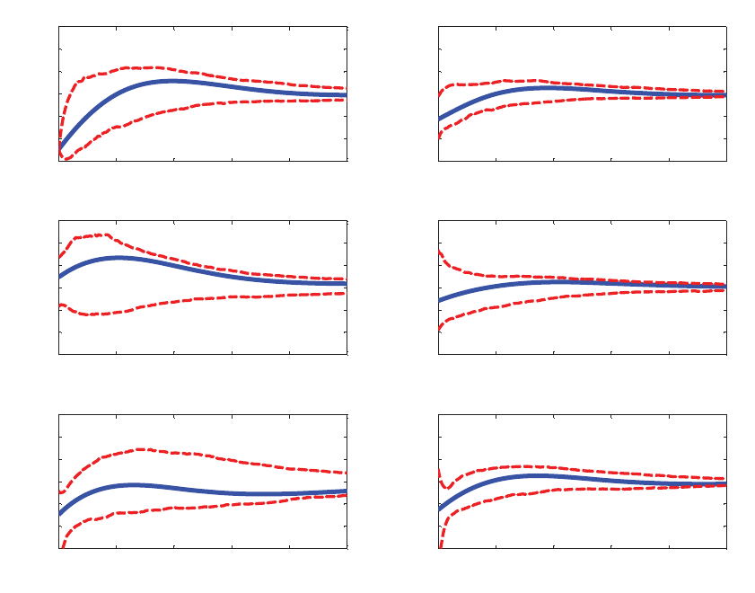
Figure 1: Estimated Impulse Responses in Baseline VAR
0 50 100 150 200 250
-0.2
-0.1
0
0.1
0.2
10 Year Treasury
0 50 100 150 200 250
-0.2
-0.1
0
0.1
0.2
2 Year Treasury
0 50 100 150 200 250
-0.2
-0.1
0
0.1
0.2
5 Year Breakeven
0 50 100 150 200 250
-0.2
-0.1
0
0.1
0.2
5-10 Year Breakeven
0 50 100 150 200 250
-0.2
-0.1
0
0.1
0.2
BAA Yields
0 50 100 150 200 250
-0.2
-0.1
0
0.1
0.2
AAA Yields
Note: Estimates of the impulse responses from monetary policy shocks onto the 6
variables in the system, from 0 to 250 days. 90 percent bootstrap confidence intervals
are also reported, constructed as described in the text. The monetary policy shock is
normalized to lower ten-year yields by 25 basis points.
24

Figure 2: Estimated Impulse Responses Using only 10 Announcement Days
0 50 100 150 200 250
-0.2
-0.1
0
0.1
0.2
10 Year Treasury
0 50 100 150 200 250
-0.2
-0.1
0
0.1
0.2
2 Year Treasury
0 50 100 150 200 250
-0.2
-0.1
0
0.1
0.2
5 Year Breakeven
0 50 100 150 200 250
-0.2
-0.1
0
0.1
0.2
5-10 Year Breakeven
0 50 100 150 200 250
-0.2
-0.1
0
0.1
0.2
BAA Yields
0 50 100 150 200 250
-0.2
-0.1
0
0.1
0.2
AAA Yields
Note: As for Figure 1, except that only the ten days highlighted in bold in Table 1 are
treated as announcement days.
25

Figure 3: Estimated Impulse Responses Using Longer Sample to Estimate VAR
0 50 100 150 200 250
-0.2
-0.1
0
0.1
0.2
10 Year Treasury
0 50 100 150 200 250
-0.2
-0.1
0
0.1
0.2
2 Year Treasury
0 50 100 150 200 250
-0.2
-0.1
0
0.1
0.2
5 Year Breakeven
0 50 100 150 200 250
-0.2
-0.1
0
0.1
0.2
5-10 Year Breakeven
0 50 100 150 200 250
-0.2
-0.1
0
0.1
0.2
BAA Yields
0 50 100 150 200 250
-0.2
-0.1
0
0.1
0.2
AAA Yields
Note: As for Figure 1, except that the reduced form VAR was estimated over the period
since Janaury 1999, as described in the text.
26

Figure 4: Estimated Impulse Responses Using Alternative VAR with MBS Rates
0 50 100 150 200 250
-0.2
-0.1
0
0.1
0.2
10 Year Treasury
0 50 100 150 200 250
-0.2
-0.1
0
0.1
0.2
2 Year Treasury
0 50 100 150 200 250
-0.2
-0.1
0
0.1
0.2
5 Year Breakeven
0 50 100 150 200 250
-0.2
-0.1
0
0.1
0.2
5-10 Year Breakeven
0 50 100 150 200 250
-0.2
-0.1
0
0.1
0.2
MBS
Note: As for Figure 1, except that the reduced form VAR included Fannie Mae current
coupon MBS yields instead of corporate bond rates.
27

Figure 5: Estimated Impulse Responses Using Alternative VAR with CDS-based corporate
yield
0 50 100 150 200 250
-0.2
-0.1
0
0.1
0.2
10 Year Treasury
0 50 100 150 200 250
-0.2
-0.1
0
0.1
0.2
2 Year Treasury
0 50 100 150 200 250
-0.5
0
0.5
5 Year Breakeven
0 50 100 150 200 250
-0.2
-0.1
0
0.1
0.2
5-10 Year Breakeven
0 50 100 150 200 250
-0.5
0
0.5
5 Year Invest. Grade CDS+Swap
Note: As for Figure 1, except that the reduced form VAR included the sum of the
Markit five-year investment grade corporate CDS index and the five-year swap rate.
Under CDS-bond arbitrage, this should theoretically be close to a corporate bond yield.
28

Figure 6: Estimated Impulse Responses in Baseline VAR using Event-Study Identification
0 50 100 150 200 250
-0.2
-0.1
0
0.1
0.2
10 Year Treasury
0 50 100 150 200 250
-0.2
-0.1
0
0.1
0.2
2 Year Treasury
0 50 100 150 200 250
-0.2
-0.1
0
0.1
0.2
5 Year Breakeven
0 50 100 150 200 250
-0.2
-0.1
0
0.1
0.2
5-10 Year Breakeven
0 50 100 150 200 250
-0.2
-0.1
0
0.1
0.2
BAA Yields
0 50 100 150 200 250
-0.2
-0.1
0
0.1
0.2
AAA Yields
Note: Estimates of the impulse responses from monetary policy shocks onto the 6 vari-
ables in the system, from 0 to 250 days. The monetary policy shocks were identified
as the first principal component of changes in bond futures quotes in intraday windows
around the events listed in Table 1. The reduced form VAR errors were then regressed
onto these monetary policy shocks and the impulse responses were computed as de-
scribed in the text. 90 percent bootstrap confidence intervals are also reported.
29

Figure 7: Estimated Impulse Responses Using only 10 Announcement Days and Event-Study
Identification
0 50 100 150 200 250
-0.2
-0.1
0
0.1
0.2
10 Year Treasury
0 50 100 150 200 250
-0.2
-0.1
0
0.1
0.2
2 Year Treasury
0 50 100 150 200 250
-0.2
-0.1
0
0.1
0.2
5 Year Breakeven
0 50 100 150 200 250
-0.2
-0.1
0
0.1
0.2
5-10 Year Breakeven
0 50 100 150 200 250
-0.2
-0.1
0
0.1
0.2
BAA Yields
0 50 100 150 200 250
-0.2
-0.1
0
0.1
0.2
AAA Yields
Note: As for Figure 5, except that only the ten days highlighted in bold in Table 1 are
treated as announcement days.
30

Figure 8: Estimated Impulse Responses Using Longer Sample to Estimate VAR and Event-
Study Identification
0 50 100 150 200 250
-0.2
-0.1
0
0.1
0.2
10 Year Treasury
0 50 100 150 200 250
-0.2
-0.1
0
0.1
0.2
2 Year Treasury
0 50 100 150 200 250
-0.2
-0.1
0
0.1
0.2
5 Year Breakeven
0 50 100 150 200 250
-0.2
-0.1
0
0.1
0.2
5-10 Year Breakeven
0 50 100 150 200 250
-0.2
-0.1
0
0.1
0.2
BAA Yields
0 50 100 150 200 250
-0.2
-0.1
0
0.1
0.2
AAA Yields
Note: As for Figure 5, except that the reduced form VAR was estimated over the period
since Janaury 1999, as described in the text.
31

Figure 9: Estimated Impulse Responses Using Event-Study Identification in Alternative VAR
with MBS Rates
0 50 100 150 200 250
-0.2
-0.1
0
0.1
0.2
10 Year Treasury
0 50 100 150 200 250
-0.2
-0.1
0
0.1
0.2
2 Year Treasury
0 50 100 150 200 250
-0.2
-0.1
0
0.1
0.2
5 Year Breakeven
0 50 100 150 200 250
-0.2
-0.1
0
0.1
0.2
5-10 Year Breakeven
0 50 100 150 200 250
-0.2
-0.1
0
0.1
0.2
MBS
Note: As for Figure 5, except that the reduced form VAR included Fannie Mae current
coupon MBS yields instead of corporate bond rates.
32

Figure 10: Estimated Impulse Responses Using Event-Study Identification in Alternative
VAR with CDS-based corporate yield
0 50 100 150 200 250
-0.2
-0.1
0
0.1
0.2
10 Year Treasury
0 50 100 150 200 250
-0.2
-0.1
0
0.1
0.2
2 Year Treasury
0 50 100 150 200 250
-0.2
-0.1
0
0.1
0.2
5 Year Breakeven
0 50 100 150 200 250
-0.2
-0.1
0
0.1
0.2
5-10 Year Breakeven
0 50 100 150 200 250
-0.2
-0.1
0
0.1
0.2
5 Year Invest. Grade CDS+Swap
Note: As for Figure 5, except that the reduced form VAR included the sum of the
Markit five-year investment grade corporate CDS index and the five-year swap rate.
Under CDS-bond arbitrage, this should theoretically be close to a corporate bond yield.
33
References
[1] Am ihud, Yak ov (2002): Illiquidit y and Stoc k Returns: Cross-Section and Time-
Series Effects, Journal of Financial Markets,5,pp.31-56.
[2] Bernan ke, Ben S. (1986): Alternative explanations of the money-incom e corre-
lation, Carnegie-Rochester Conferen ce Series on Public Policy, 25, pp.49-99.
[3] Bernan ke Ben S. and Kenneth N. Kuttner (2005): W h at Exp lains the Stock
Market’s Reaction to Federal Reserve P olicy? , Journal of Financ e, 60, pp.1221-
1257.
[4] Christian o, La w r ence J., Martin Eichenbaum and Charles L. Evans (1996): The
Effects of Mon etar y Policy Shoc ks: Evidence from the Flo w of Funds, Review of
Eco n o mics and Statistic s, 78, pp.16-34.
[5] D’A m ico , Stefan ia and Thomas B. King (2010): Flo w and Stock Effects of Large-
Scale Treasury Purchases, Finance and Economics Discussion Series 2010-52.
[6] Doh, Taeyoung (2010): The Efficacy of Large-Scale Asset Purchases at the Zero
Low er Bound, Federal Reserve Bank of Kansas Cit y Economic Review.
[7] Faust, Jon, Eric T. Sw a nson and Jonathan H. Wright (2011): Iden tifying VARs
Based on High Frequency Futures Data , Journal of Monetary Economics,51,
pp.1107-1131.
[8] Gagnon, Joseph , Matthew Raskin, Julie Remac he and Brian Sac k (2010): Large-
Scale Asset Purc hases by the Federal Reserv e: Did They Work?, Federal Reserv e
Bank of New York Staff Report 441.
[9] Gürkaynak, Refet S., Brian Sack and Eric T. Sw anson (2005): Do Actions Speak
Louder Than Words? The Response of Asset Prices to Monetary P olicy Actions
and Statements, International Journal of Central Banking,1,pp.55-93.
[10] Gürkay nak , Refet S., B rian Sack and Jonathan H. Wright (2007): The U.S.
Treasury Yield Curve: 1961 to the Presen t, Journal of Monetary Economics,54,
pp.2291-2304.
[11] Gü rkayna k , Refet S., Bria n Sack and Jonathan H. Wright (2010): The TIP S yield
curve and Inflation Compensation, Am eric an Economics Journal,2,pp.70-92.
[12] Hamilton, James D. and Jing Wu (2010): Th e Effectiveness of Alternative Mone-
tary Policy Tools in a Zero Lo wer Bound Environm ent, w orking paper, Un iversit y
of California, San Diego.
[13] Hancoc k, Diane and Wayn e P assm or e (2011): Did the Federal Reserve’s MBS
Purchase Program Lo wer Mortgage Rates?, Finance and Econom ics Discussion
Series, 2011-01.
34
[14] Kohn, Don (2009): Monetary Policy in the Financial Crisis, speech.
[15] Krishnam urth y, Arvind and Annette Vissing-Jorgenson (2011): The Effects of
Quantitative Easing on Long-term In terest Rates, working paper, Northw estern
Universit y.
[16] Kilian, Lutz (199 8): Small-Sa m ple Confidence In tervals for Impulse Response
Functions, Review of Ec onomics and Statistics, 80, pp.218-230.
[17] Kuttn er, Kenneth N. (2001): Monetary Policy Surprises and Interest Rates: Evi-
dence from the Fed Funds Futures Market, Journal of Monetary Economics,47,
pp.523-544.
[18] Modigliani, Franco and Richard Sutch (1966): Innovations in Interest Rate Pol-
icy, American Econom ic Review, 52, pp.178-97.
[19] Modigliani, Franco and Richard Sutch (1967): Debt Managemen t and the Term
Structure of Inter est Rates: An Empirical Analysis of Recen t Experience, Journal
of Politic al Ec onomy, 75, pp.569-89.
[20] Neely, Christo pher (2010): The Large-Scale Asset Purchases Had Large In tern a-
tional Effects, wo rking paper, Federal Reserve Bank of St. Louis.
[21] Politis, Dimitr is N. and Joseph P. Rom ano (1994): The Stationary Bootstrap,
Jou rn al of the American Statistical Association, 89, pp.1303-1313.
[22] Rigobon, Roberto (2003): Iden tification Throug h Heteroskedasticit y, Review of
Eco n o mics and Statistic s, 85, pp.777-92.
[23] Rigobon, Roberto and Brian Sack (2003): Measuring the Response of Monetary
P olicy to the Stock Mark et, Quarterly Journal of Economics, 118, pp.639-669.
[24] Rigobon, Roberto and Brian Sack (2004): The Impact of Monetary P olicy on
Asset Prices, Journal of Monetary Economics, 51, pp.1553-1575.
[25] Rigobon, Roberto and Brian Sac k (2005). The Effects of War risk on US Financial
Markets, Journal of Banking and Finance, 29, pp.1769-1789.
[26] Sims, Chr istoph er A. (1980): Macroeconomics and reality, Econom etrica,48,pp.
1—48.
[27] Sw anson, Eric T. (2011): Let’s Twist Again: A High-Frequency Ev en t-Study
Analysis of Operation Twist and Its Implications for QE2 , BrookingsPaperson
Econ omic Activity,forthcoming.
[28] Vayanos, Dimitri and Jean-Luc Vila (2009): A Preferred-Habitat Model of the
Term-Stru cture of In ter est Rates, working paper, London Sc hool of Economics.
35
