
WHITE PAPER
OFFICE OF MANAGEMENT AND BUDGET
CLIMATE RISK EXPOSURE:
AN ASSESSMENT OF THE FEDERAL GOVERNMENT’S FINANCIAL RISKS TO
CLIMATE CHANGE
April 2022

Table of Contents
Introduction ..................................................................................................................................... 1
Crop Insurance ................................................................................................................................ 9
Coastal Disasters ........................................................................................................................... 17
Federal Healthcare Spending ........................................................................................................ 26
Federal Wildland Fire Suppression Expenditures......................................................................... 35
Federal Facility Flood Risks ......................................................................................................... 43
Flood Insurance ............................................................................................................................. 50
References ..................................................................................................................................... 56
Technical appendix: Climate Risk Exposure: Coastal Disasters .................................................. 63
Technical Appendix: Climate Risk Exposure: Federal Wildfire and Suppression Expenditures.
Research and Development, USDA Forest Service
,
..................................................................... 66
CLIMATE RISK EXPOSURE: AN ASSESSMENT OF THE FEDERAL GOVERNMENT’S FINANCIAL RISKS TO CLIMATE CHANGE
1
Introduction
The climate crisis poses a serious threat to the United States economy and human welfare, with a
narrowing timeframe to invest in opportunities to avoid the most catastrophic impacts. Extreme
weather events can be exacerbated by climate change, disrupting supply chains, and flooding
made worse by sea level rise can destroy critical infrastructure. As a smaller subset of these
impacts, climate change threatens the Nation’s fiscal health. The Fourth National Climate
Assessment (NCA4) notes that:
Climate change creates new risks and exacerbates existing
vulnerabilities in communities across the United States, presenting
growing challenges to human health and safety, quality of life, and the
rate of economic growth.
The impacts of climate change on businesses and communities are broad; escalating costs, and
lost revenue as a direct or indirect result of a changing climate is significant and varied. Across
the United States, estimated damages from a subset of storms, floods, wildfires, and other
extreme climate-related weather events have already grown to about $120 billion a year over the
past five years (Smith, 2021). Some of the most severe harms from climate change will fall
disproportionally upon socially vulnerable populations, including racial and ethnic minority
communities (EPA, 2021). The Federal Government plays a critical role in helping American
families, businesses, and communities recover from the impacts of extreme weather events –
often acting as an insurer of last resort. Communities and businesses also face both immediate
hazards, along with increasing risks over time, such as sea level rise. For instance, the Federal
Government must ensure that Americans have access to housing and healthcare that is safe and
affordable as well as access to critical transportation and communication infrastructure. Climate
change increases the need for Federal support in these areas.
As broad economic damages from climate change grow, so does the impact of the climate crisis
on the Federal budget. the Federal Government’s budget is directly and substantially at risk from
expected lost revenues and increasing expenditures due to climate change damages in coming
decades, such as increasing costs from physical damages to our nation’s infrastructure and
healthcare expenditures, the instability of certain subsidized insurance programs, and
accelerating instability that threatens global security.
To help address threats that climate change poses to the economy, President Biden signed the
“Executive Order on Climate-Related Financial Risk” (“Executive Order”) on May 20th, 2021.
Section 6(b) of the Executive Order directs “[t]he Director of Office of Management and Budget
and the Chair of the Council of Economic Advisors, in consultation with the Director of the
National Economic Council, the National Climate Advisor, and the heads of other agencies as
appropriate, [to] develop and publish annually, within the President’s Budget, an assessment of
the Federal Government’s climate risk exposure.” This paper assesses several areas where the
Federal Government may experience significant climate change-associated risk and highlights
some steps the Federal Government is taking to address those risks.

CLIMATE RISK EXPOSURE: AN ASSESSMENT OF THE FEDERAL GOVERNMENT’S FINANCIAL RISKS TO CLIMATE CHANGE
2
Although the presence of risk to the U.S. economy and to the Federal budget across these and
other exposure points is clear (and supported by a large body of scientific evidence), we remain
in the early stages of quantifying the total potential risk for American taxpayers and Federal
programs. In several critical areas, quantitative projections of specific climate impacts are not yet
available. Additionally, where climate impact measures do exist, estimating the impact on the
Federal budget can be challenging due to the need to tie those risks to future decisions (e.g.,
estimating the extent to which the U.S. government will provide disaster aid or take on other
liabilities). The report examines the Federal Government’s climate risk exposure through six
program-specific assessments that consider a handful of the out-year potential damages to these
programs: crop insurance, coastal disasters, Federal healthcare, Federal wildland fire
suppression, Federal facility flood risk, and flood insurance.
1
By reviewing the major impact
categories in the NCA4 and examining data limitations of future risk for Federal programs, it is
clear that significant climate risks are understood and apparent, but they are unable to be
quantified at this time. The assessments included in this paper and projected risks that are
quantified are helpful in approximating the order of magnitude of potential impacts of climate
change on the Federal budget, in these six areas, but are subject to limitations and uncertainty.
A preliminary OMB/CEA report on this topic was published in 2016, which estimated that
annual Federal expenditures could increase by $34-$112 billion per year by later century due to
the impacts of climate change, along with significant potential for economic and Federal revenue
losses (OMB, 2016). This assessment expands upon, and updates, that 2016 assessment.
Expenditure Impacts
Several limitations exist when projecting Federal expenditures. The horizon for most projections
in Federal budgeting is 10 years; that horizon reflects a balance between the importance of
considering both the current and future implications of budget decisions made today, and a
practical limit on the construction of detailed budget projections for years in the future. Many
impacts of climate change are expected to continue to worsen far beyond this 10-year horizon,
and climate assessments (including those conducted in this paper) are often based on scenarios
going to the mid- or late-century – well within the lifetimes of today’s youngest Americans.
Nonetheless, it is informative to regularly model future conditions with the best available data to
provide a relative scale of impact on future expenditures. The six individual assessments
described in this paper reflect only a small portion of potential future financial risks to the
Federal Government, but clearly illustrate that Federal financial risks will increase and create a
demand for increased Federal expenditures.
Table 1 below shows estimates of recurring, annual expenditures (as impacted by climate
change). The increased expenditures from these assessments total between an additional $25
billion to $128 billion per year by late century. These estimates represent only a narrow portion
1
The Federal Government’s exposure to climate risk is broader than the six assessments conducted for this paper.
For further discussion of additional areas of Federal financial risks due to climate change, see the FY 2023
Analytical Perspectives chapter: Federal Budget Exposure to Climate Risk.
https://www.whitehouse.gov/wp-
content/uploads/2022/04/ap_21_climate_risk_fy2023.pdf

CLIMATE RISK EXPOSURE: AN ASSESSMENT OF THE FEDERAL GOVERNMENT’S FINANCIAL RISKS TO CLIMATE CHANGE
3
of the full financial risks of climate change to the Federal Government. Several impacts are not
quantified in this report due to data limitations and other obstacles. For instance, impacts on
national security; transportation, energy, and water infrastructure; ecosystem services; and some
types of health impacts are not quantified due to the nascent nature of conducting these
assessments. However, opportunities exist to expand expenditure assessments in future years to
include additional topics and a broader set of modeling.
Table 1. Summary of Spending Increases for Quantified Climate Risk Exposure of
Assessed Programs, in billion dollars (2020$)
a
a
“Lower” estimates are largely based on assessments assuming Representative Concentration Pathway (RCP) 4.5,
which the NCA4 framed in 2018 as a "lower" scenario with less warming - generally associated with lower
population growth, more technological innovation, and lower carbon intensity. “Higher” estimates are largely based
on assessments assuming RCP8.5, which the NCA4 frames as a "higher" scenario - generally associated with higher
population growth, less technological innovation, and higher carbon intensity.
b
The crop insurance analysis was only conducted for late century.
c
The median of all wildland fire suppression simulations are used in the “Mean” column, so outliers in the “Higher”
scenario are not overemphasized in the results.
d
Several Federal financial risks are not included in this table due to the nascent ability to quantify future
expenditures in this field. Some other future expenditures, such as flood insurance are not expected to increase
because rate setting policies yield actuarially fair premiums with the ability to adjust as climate conditions change.
e
The science of estimating Representative Concentration Pathways (e.g. RCP4.5 and RCP8.5) has evolved since
NCA4 was released in 2018. RCP8.5, for instance has been viewed by some researchers as an extreme scenario.
specific climate scenarios, and time periods can vary across this paper's assessments due to differences in available
studies, datasets, and models. As a result, findings are comparable across risk assessments at an order-of-magnitude
scale.
Mean Lower Higher Mean Lower Higher
Mid Centuryᵉ
Late Century
Crop Insuranceᵇ
$1.2 $0.3 $2.1
Wildland fire Suppressionᶜ
$1.7 $0.8 $2.3 $3.7 $1.6 $9.6
Health Impacts
$1.0 $0.2 $1.8 $11.3 $0.8 $21.9
Coastal Disasters
$14.6 $4.4 $32.5 $49.6 $21.9 $94.3
Totalᵈ
$17.3 $5.4 $36.6 $65.8 $24.6 $127.9
$0.0
$1,000.0
$2,000.0
$3,000.0
$4,000.0
$5,000.0
$6,000.0
$7,000.0
$8,000.0
$9,000.0
$10,000.0
$0
$20
$40
$60
$80
$100
$120
$140
Billion dollars
(2020$)
NA
NA
CLIMATE RISK EXPOSURE: AN ASSESSMENT OF THE FEDERAL GOVERNMENT’S FINANCIAL RISKS TO CLIMATE CHANGE
4
Estimated climate-related financial costs reach into the tens of billions per year by mid-century
and grow into late-century. Climate-related costs in the assessed areas will also likely vary
significantly from year to year, for instance the case of extreme weather events is expected to
become more frequent and impactful in the years to come. This variation makes future planning
and budgeting even more challenging and can create a reliance on supplemental appropriations
outside of the annual budget process.
Revenue Impacts
Climate change is projected to reduce economic output in the United States and across the globe
(Auffhammer, 2018). Because a large proportion of Federal revenue comes from labor and
capital income taxes, and because lower output means lower aggregate labor and capital income,
reduced output in the United States means lost revenue for the Federal Government under current
tax policies. The Intergovernmental Panel on Climate Change (IPCC)’s most recent midrange
projection under their very high greenhouse gas (GHG) emissions scenario suggests that
warming of four and a half degrees Celsius over preindustrial levels could occur by 2100 if
global emissions are allowed to continue unabated. However, climate commitments, from both
governments and private industry, and technological advancements that have been implemented
worldwide indicate that warming may be limited to just over three degrees Celsius under
intermediate GHG emissions scenarios (IPCC, 2021; NGFS, 2021). One way economists have
tried to estimate the economic damages from climate change is by estimating the correlation
between macroeconomic activity and observed temperatures. Economists using this approach
estimate that economic damages from warming between two and a half and four and a half
degrees Celsius range from two to 23 percent of global gross domestic product (GDP) each year
by 2100 (Kalkuhl and Wenz, 2020; NGFS, 2021; Newell, Prest and Sexton 2021; Burke et
al. 2015). The distributions of these damage estimates are often not symmetric, with the same
studies producing upper-end extreme outcomes at the 95
th
percentile that range from 8.5 percent
to over 50 percent of global GDP. One of the economic models places the estimate of annual
damages from warming of three degrees Celsius at the 95
th
percentile at about 10 percent of U.S.
GDP by the end of the century (NGFS, 2021).
A number of factors affect the magnitude of such estimates, including the known uncertainties
not captured. For example, the estimates do not account for important long-term factors that
remain difficult to estimate using short-term variations in weather, both in terms of changes to
the environment and monetarily, such as biodiversity loss, ocean acidification, and sea level rise
(Dell, Jones, and Olken, 2014). Tipping points associated with non-linear changes in the climate
and unprecedented events, like ice sheet disintegration and thawing permafrost, are also not
captured in projections based on historical relationships between climate change and physical
outcomes (Dietz et al., 2021). In addition, there is a lot of variation across current models that
stem from uncertainty as to whether economic damages accrue to the level of GDP, the growth
rate of GDP over time, or both. A small change in the growth rate can accumulate into large
annual damages over a longer horizon, pushing the expected economic damages towards the top
of the range of estimated impacts. For example, research suggesting that economic productivity
is nonlinear relative to temperature changes—that there are significant negative temperature

CLIMATE RISK EXPOSURE: AN ASSESSMENT OF THE FEDERAL GOVERNMENT’S FINANCIAL RISKS TO CLIMATE CHANGE
5
threshold effects on productivity in affected sectors—indicates that the estimates of climate
change on economic growth rates would result in global GDP being reduced by over 20 percent
in 2100 in the high emissions RCP 8.5 scenario (Burke et al., 2015). In contrast, Newell, Prest
and Sexton (2021) assess the impact of climate change on GDP levels and show that in 2100,
using the same high emissions scenario, global GDP is reduced by only 1 to 3 percent.
The uncertainty of economic damage projections is compounded when attempting to estimate the
associated potential for lost U.S. Federal revenue. The exercise relies on difficult assumptions
about the impact of economic losses on U.S. GDP and Federal revenue’s sensitivity to U.S.
GDP. For example, as discussed above, economic losses are commonly expressed as a percent of
output and losses that occur in the form of non-market losses (e.g., premature mortality or
biodiversity loss) do not directly translate into lost GDP—or Federal revenue.
In a scenario resulting in three degrees Celsius warming, the top end of the confidence interval
(95th percentile) of GDP losses would result 7.1 percent lower Federal revenue by 2100 --
equivalent to approximately $2 trillion per year in today’s dollars.
2
These estimates are the
product of a simple extrapolation from leading economic loss projections and should be
interpreted as one point in a range of possible revenue losses, rather than precise estimates.
Overview of assessments
Climate-related financial risks can affect the U.S. economy through two channels. The first
involves physical risks, arising from damage to property, infrastructure, human health, and land.
The second, transition risk, results from changes in policy, technology, and consumer and market
preferences during the adjustment to a lower-carbon economy. Although the presence of risk to
the U.S. economy and to the Federal budget across these and other exposure points is clear, and
supported by a large body of scientific evidence, quantifying the total potential risk for American
taxpayers and Federal programs remains in its early stages. Also, quantitative projections of
specific climate impacts to related Federal program expenditures are not yet available in several
critical areas, such as Federal financial infrastructure risks, national security risks, and risks to
ecosystems. Additionally, where climate impact measures do exist, estimating the impact on the
Federal budget can be challenging due to the need to tie those risks to future decisions (e.g.,
estimating the extent the U.S. government will provide disaster aid or take on other liabilities).
The projections we do have are useful in approximating the order of magnitude of potential
impacts of climate change on the Federal Budget but are still subject to significant limitations
and uncertainty.
These assessments complement execution of the Executive Order on Tackling the Climate Crisis
at Home and Abroad, as well as supporting budget priorities related to climate adaptation and
resilience, by focusing on long-term risks to the United States’ Federal ledger. Much of the work
associated is also complemented by, and benefits from, the National Climate Assessment.
2
The 95
th
percentile estimate used here is projected by NGFS under their Current Policies scenario. The NGFS Current Policies
scenario assumes warming of over three degrees Celsius above pre-industrial averages. Economic damages for that amount of
warming are estimated using the results from Kalkuhl and Wenz (2020) and are roughly 10 percent of GDP in 2100.

CLIMATE RISK EXPOSURE: AN ASSESSMENT OF THE FEDERAL GOVERNMENT’S FINANCIAL RISKS TO CLIMATE CHANGE
6
While a robust set of scientific studies and models of the global risks and impacts of climate
change exist, our current understanding of the fiscal risks of climate change to the Federal
Government is nascent, limited in scope, and subject to significant uncertainty. For instance,
many models are based on known conditions, while the largest future climate impacts will be
from previously low probability events that are now becoming normalized. Modeling these high-
impact events can create wide ranges of potential cost impacts. However, the available evidence
thus far indicates the fiscal risks to the Federal Government could be very significant over the
course of this century without ambitious action to reduce GHGs and adapt our communities to a
changing climate.
A preliminary, related OMB/CEA report, Climate Change: The Fiscal Risks Facing the Federal
Government, was published in 2016, along with an Analytical Perspectives chapter in the FY
2017 Budget. The 2016 report concluded that annual Federal expenditures could increase by $34
to $112 billion per year by later this century due to the impacts of climate change, along with
significant potential for economic and Federal revenue losses. The assessment noted limitations
in producing these estimates and did not attempt to assess macroeconomic impacts of climate
change.
This white paper builds on the work done for the 2016 report. In this white paper, prior
assessments were either updated, expanded upon, or reworked using updated modeling
assumptions. In many subject areas, more recent relevant Federal and academic modeling or
analyses have been published, which have been utilized to advance and improve the assessments
conducted for this white paper. OMB selected six key areas to conduct individual assessments in
this white paper. These areas were chosen because each has strong links to the Federal Budget,
are clearly vulnerable to the impacts of climate change, and are topics which have scientific or
economic data available that can produce quantitative modeling of impacts. The six areas are:
crop insurance, coastal disasters, Federal healthcare spending, Federal wildland fire suppression
expenditures, Federal facility flood risks, and flood insurance. In each of these areas, OMB
worked with experts across the Federal Government to leverage the best available quantitative
modeling to estimate key potential effects of climate change and the associated financial risks to
those Federal programs.
Each risk assessment draws either on findings from the best available scientific and economic
literature or new analysis that uses existing models and datasets. The assessments generally
compare current annual spending without further climate change to projected spending based on
future scenarios utilized by the National Climate Assessment and International Panel on Climate
Change. The assessments draw upon Representative Concentration Pathways, or RCPs, which
are widely used in the climate research community to describe different climate futures and are
based on the volume of greenhouse gases emitted. RCPs form the foundation for the majority of
recent climate-related modeling efforts. The Fourth NCA largely focuses on RCP8.5 and RCP4.5
for framing purposes.
3
This paper attempts to follow the framing of the NCA by using data and
modelling references from RCP4.5 and RCP8.5 when climate projection models and data are
available. However, specific climate scenarios, and time periods can vary across this paper's
3
RCP4.5 is framed as a "lower" scenario with less warming and is generally associated with lower population growth, more
technological innovation, and lower carbon intensity. RCP8.5 is framed as a "higher" scenario and is generally associated with
higher population growth, less technological innovation, and higher carbon intensity.
CLIMATE RISK EXPOSURE: AN ASSESSMENT OF THE FEDERAL GOVERNMENT’S FINANCIAL RISKS TO CLIMATE CHANGE
7
assessments due to differences in available studies, datasets, and models. As a result, findings are
comparable across risk assessments only at the order-of-magnitude scale. Several of the
assessments compare an unmitigated climate to different potential futures.
In addition, due to limitations in available models and the uncertainty inherent in projecting
several decades into the future, the results of these assessments should be interpreted as
indicative of the order of magnitude of potential impacts of climate change on Federal spending
in the studied scenarios. Actual future impacts will vary depending on a wide range of factors
such as population and income growth, policy changes, technological development, changing
behavior—including adaptive responses—and the magnitude and pace of further climate change.
Generally, the assessments do not attempt to fully represent the potential for adaptation or policy
changes to attenuate fiscal impacts. For example, adaptation investments or assumptions are
often not modeled or forecasted.
Along those lines, the overall scope of the paper is not comprehensive. Substantial financial risks
to national security, transportation and water infrastructure, ecosystem services, and several other
climate impacts are not assessed in this paper. Also, the breadth of each individual assessment
offers a fraction of the potential quantified risks within that topic. For instance, morbidity
estimates are modeled for only a handful of the health risks caused by climate change in the
healthcare assessment. It is highly plausible that the actual climate-related financial risks to the
Federal Government are much larger than those that are presented in this paper.
Future opportunities to better understand financial risks
As academic literature on climate science and economics continue to advance, further
collaboration between OMB, CEA, and other key Federal agencies will be necessary to ensure
that the understanding of climate change risks facing the Federal Budget becomes more
comprehensive. The “Executive Order on Climate-Related Financial Risk” calls for an annual
assessment of the Federal Government’s climate risk exposure. By more regularly and
consistently incorporating climate-related financial risk planning into the budget process, the
executive branch will be better suited to assess risks.
The FY 2023 President's Budget and agencies' Congressional Justifications highlight several
budgetary requests that will help reduce the Federal Government’s long-term fiscal exposure to
climate-related financial risk. Near-term Federal investments to both mitigate greenhouse gas
emissions and adapt to future climate scenarios can help reduce the future costs identified in this
paper but will require both Congressional appropriations and Federal implementation. Several
near-term investments to reduce future climate risks are presented in the FY 2023 President’s
Budget. While investments are expected to reduce the Federal Government's exposure to future
climate-related financial risks, more work is needed to identify and quantify the impact of factors
that can mitigate or compound climate change fiscal risk. Investments in adaptation, for instance,
can significantly reduce future risk exposure. At times, higher up-front adaptation costs will save
taxpayers and the Federal Government in the long-term. On the other hand, business as usual
investments that are more prone to the risks from climate change could further exacerbate future
risks. Better understanding and attempting to quantify factors like these as they relate to Federal
CLIMATE RISK EXPOSURE: AN ASSESSMENT OF THE FEDERAL GOVERNMENT’S FINANCIAL RISKS TO CLIMATE CHANGE
8
budget formulation is important for taking steps to mitigate the broad and urgent financial crises
the Federal Government could face.

CLIMATE RISK EXPOSURE: AN ASSESSMENT OF THE FEDERAL GOVERNMENT’S FINANCIAL RISKS TO CLIMATE CHANGE
9
Crop Insurance
As mentioned in NCA4, climate change is anticipated to shift agricultural production regions
(USGCRP, 2018). Average crop yields for most major commodities are projected to decline due
to higher temperatures, as well as climate-change induced drought intensification and
increasingly frequent natural disasters such as flooding. Particularly, crops which are planted in
the spring—such as corn, soybeans, and sorghum—are more likely to experience declines in
productivity due to excessive heat and dryness during summer (Gowda et. al, 2018). Crops vary
in their ability to handle high temperatures and drought. For example, soybeans are more
sensitive to extreme heat relative to corn; therefore, soybeans are projected to experience larger
declines in crop productivity from climate change compared to corn (Crane-Droesch et al.,
2019). However, crops, such as winter wheat and barley, may experience increased yields from
higher temperatures in the spring since these crops are planted in the fall and harvested in early
summer. In the Western part of the United States, where wildfire frequency and intensity are
anticipated to increase, wine grape production may experience losses directly from fire and
$9.4B
$9.8B
$11.5B
$0
$2
$4
$6
$8
$10
$12
$14
Baseline RCP 4.5 RCP 8.5
Billion dollars (2020$)
Projected Change in Total Annual Premium Subsidies for the
Year 2080, billion dollars (2020$)
Corn Soybeans Wheat
USDA found that Federal expenditures on crop insurance premium subsidies are expected to
increase 3.5 to 22 percent due to climate change-induced crop losses by the late-century
Under RCP 4.5, the subsidies for crop insurance premiums would be about 3.5 percent
higher compared to a climate similar to that of the recent past—an increase of roughly $330
million/year in 2020 dollars by the late century. Under RCP 8.5, the projected increase in
crop insurance premium subsidies is 22 percent—an approximate increase of $2.1 billion per
year (2020$) by the late-century.

CLIMATE RISK EXPOSURE: AN ASSESSMENT OF THE FEDERAL GOVERNMENT’S FINANCIAL RISKS TO CLIMATE CHANGE
10
indirectly from smoke taint
4
(Krstic, Johnson, and Herderich, 2015). While there could be some
benefits to climate change, models overall project a negative impact on crop production.
Previous research has estimated that county-level temperature trends caused 19% of the national-
level Federal crop insurance gross indemnities from 1991 to 2017 (Diffenbaugh et al., 2021).
The Federal Crop Insurance Program (FCIP) provides subsidized insurance for losses from
unexpected decreases in crop yields or revenue caused by natural perils. The program operates
through a public-private partnership between the Federal Crop Insurance Corporation (FCIC)—
the Federal Government entity—and Approved Insurance Providers (AIPs)—the private sector
entities. The Risk Management Agency (RMA) of the U.S. Department of Agriculture (USDA)
oversees operation of the FCIP, as directed by the FCIC Board of Directors (7 U.S.C. § 1508).
The FCIP is subsidized through insurance premium subsidies and, for the private sector
implementation, subsidies for administrative and overhead expenses (7 U.S.C. § 1508(e)).
Premium subsidy is based on a percentage of the total insurance premium, such that the total
premium is the sum of the premium subsidy and the “farmer-paid” premium (Rosch, 2021).
Additionally, the program requires that producers cannot be excluded from the program on the
basis of risk, assuming the producer is using good farming practices for producing their crop. In
2021, farmers paid 37% of the total crop insurance premium, with the remaining 63% being
subsidized by the Federal Government (Risk Management Agency, 2021). Also, the FCIC
provides reinsurance— insurance for insurance providers when catastrophic events result in high
indemnities paid to insurance policyholders—to the AIPs through the Standard Reinsurance
Agreement (SRA), which provides the terms and conditions under which FCIC and the AIPs
share in premiums and losses. When the FCIC’s share of losses exceeds its share of premiums
per the terms of the SRA, there is an additional cost to the Federal Government in the form of
“underwriting losses” (Rosch, 2021).
While the Federal crop insurance program existed in pilot form from the 1930s through the
1970s, the permanent Federal crop insurance program was established by the Federal Crop
Insurance Act of 1980. The program did not gain traction until after the 1994 Crop Insurance
Reform Act (Risk Management Agency, 2013), which significantly increased premium subsidies
and introduced the catastrophic level of coverage. As premium subsidies increased, participation
expanded, and underwriting was refined, the program’s actuarial performance improved. Since
the expansion of the program, the FCIP portfolio has grown in diversity in crops and geographic
location. Over 100 agricultural commodities had crop insurance policies available and the
liability for the program totaled $136.6 billion with premium subsidies totaling $8.6 billion in
2021. (Risk Management Agency, 2021). By expanding to include a greater diversity of
locations and crops, the FCIP is able to maintain actuarial soundness, which means, on average,
that unsubsidized (total) insurance premiums will equal gross insurance indemnities
5
. In other
words, risk is accurately reflected in insurance premiums. However, maintaining actuarial
soundness does not mean that the program costs will be constant. For example, climate change
could impact the costs of the program.
4
Smoke taint causes crops to become unpalatable due to an “ash-y” flavor. The issue is particularly notable in wine grapes.
5
Gross indemnities are equal to the indemnities that farmers receive from the insurance policy in the event of a crop loss. Net
indemnities are equal to the gross indemnities minus the farmer-paid insurance premium. Note the definition of “actuarially
sound” excludes administrative costs.

CLIMATE RISK EXPOSURE: AN ASSESSMENT OF THE FEDERAL GOVERNMENT’S FINANCIAL RISKS TO CLIMATE CHANGE
11
To examine how the program cost could change over time, researchers from USDA’s Economic
Research Service (ERS) developed a series of models to project the increase in Federal
Government outlays associated with crop insurance premium subsidies towards the end of this
century (Crane-Droesch et al., 2019). While the Federal Government subsidizes premiums,
administrative costs, and underwriting losses, the majority of the outlays for FCIP are associated
with the premium subsidies. For example, for crop year 2019, 76.5% of the program costs were
from premium subsidies (Risk Management Agency, 2021).
Risk Assessment
To develop projected costs of the FCIP, there are several modeling components. The modeling
assumes that the policy variables, such as the design of the crop insurance program and the
current subsidy rates, remain constant. The potential changes in costs stem from changes in the
total premiums, which are dependent on acreage, average yields, average prices, yield risk, and
price risk. Since premium subsidies are a percentage of the total premiums, increases or
decreases in the total premiums will result in the premium subsidies increasing or decreasing as
well. Given that the majority of crop insurance liability
6
(and the most robust data) is for row
crops, the researchers focused on the three most widely grown crops in the United States: corn,
soybeans, and wheat (Crane-Droesch et al. 2019). These three crops account for 60% of total
crop insurance liability (Risk Management Agency, 2021).
The model components are as follows:
• Yields: The researchers established historical relationships between crop yield (crop
production per acre) and weather variables, such as air temperature, precipitation and
growing degree days
7
. The models, utilizing the historical data, are then used to project
yields out to the end of the century with input from five commonly-used General
Circulation Models (GCMs), which represent a wide range of outcomes. GCMs use
information relating to greenhouse gas emissions from RCPs to generate projections of
climate variables.
The researchers examined two different warming scenarios, one that is a high-emissions
“worse-case” scenario (RCP8.5) and another that projects lower warming (RCP4.5). For
the time period examined, the researchers compare the total expected insurance premiums
in 2080 under each scenario to a baseline climate (1981-2013) scenario using a forty-year
period in the GCM output (2060-2099) to capture yield risk.
• Economic: The projected average yields are then entered in ERS’s Regional
Environment and Agriculture Programming Model (REAP), which is an economic model
that simulates producers’ crop choice, planted acres, and crop prices under the various
yields produced by the different climate scenarios.
6
Liability is defined by a percentage selected by the producer (typically between 50%-85%) multiplied by the crop price,
expected yield, and acreage insured.
7
Growing degree days are an agronomic measure of how many days are suitable for plant growth based on whether the
temperature exceeds a certain base threshold.

CLIMATE RISK EXPOSURE: AN ASSESSMENT OF THE FEDERAL GOVERNMENT’S FINANCIAL RISKS TO CLIMATE CHANGE
12
• Policy: From the crop price and yield distributions that are outputted from REAP, the
researchers project the crop insurance premiums and subsidies. The FCIP has multiple
types of crop insurance, most of which either insures the producer for a certain level of
yield per acre or crop revenue per acre. The researchers’ calculations assume the most
popular form of crop insurance for corn, soybeans, and wheat, called Revenue Protection
(RP), for all insured acreage in the projections. RP provides farmers with a guaranteed
percent of their anticipated revenue (Risk Management Agency, n.d.). The anticipated
revenue is based on historical yields of the producer and the greater of the projected price
at the beginning of planting season or the price during harvest time (Crane-Droesch et al.
2019). In 2020, 90.5% of FCIP liability for corn, wheat, and soybeans was RP (Risk
Management Agency, 2021).
The analysis assumes that the FCIP will maintain actuarial soundness in the future; this
assumption is supported by recent historical data (Crane-Droesch et al. 2019). Over the
last 20 years, the national average loss ratio
8
has stayed close to 1. A loss ratio of 1
indicates that an insurance program is actuarially sound (Risk Management Agency,
2021).
The research shows there is a great amount of uncertainty under the different warming scenarios
and GCMs; however, there are general trends that can be expected. The analysis shows that
generally crop yields will decrease under the warming scenarios. To provide context for the
changes in the cost of the program, we first observe how yields and planted acreage are
anticipated to change near the end of the century.
Due to climate change, overall, acreage is anticipated to decline. Decreases in non-irrigated
acreage more than offset increases in irrigated acreage. Dryland (non-irrigated) corn planted
acreage is expected to decline throughout the Midwest with the largest declines in southern
Nebraska and northern Kansas. Irrigated acres of corn in the Midwest, particularly eastern
Nebraska and western Iowa are anticipated to increase. The trends in soybeans are similar to the
trends in corn. In particular, a higher fraction of soybean acreage in the Delta region
9
will be
irrigated. Wheat acreage is less concentrated in the Midwest compared to corn and soybeans: A
sizable portion of wheat production occurs in the western United States, especially in
Washington, Oregon, Idaho, and Montana. Large declines in dryland wheat acreage are
anticipated in Washington and Kansas. The increases in irrigated wheat acreage are primarily
projected in Oregon and Washington through the Dakotas and the Delta region. As an exception,
as the climate changes in northeastern North Dakota, dryland acreage for wheat is projected to
increase there.
Generally, these projections show declining yields caused by climate change. The largest
declines in non-irrigated yields, in terms of percentages, are projected in the southeastern United
States. There are expected increases for irrigated corn yields in Montana, Wyoming, and
8
The loss ratio is equal to gross indemnities divided by unsubsidized insurance premiums.
9
The Delta region is composed of Arkansas, Mississippi, and Louisiana. This region is as defined by the Economic Research
Service Farm Production Regions.
CLIMATE RISK EXPOSURE: AN ASSESSMENT OF THE FEDERAL GOVERNMENT’S FINANCIAL RISKS TO CLIMATE CHANGE
13
Colorado; however, these increases are not anticipated to be substantial. Likewise, there are
some projected increases for irrigated soybeans in southwestern North Dakota. The changes to
wheat are more variable. Both dryland and irrigated wheat yields are projected to increase in the
Dakotas and Montana, while substantial yield declines are anticipated in Arizona and New
Mexico.
In addition to the change in production—the product of yield and acreage—both yield risk and
price risk are projected to change due to climate change. The authors at the ERS report risk using
a measure called the “coefficient of variation” (CV), which is the variability (standard deviation)
divided by the average (mean). This provides an appropriate measure for looking at percentage
changes under different scenarios and GCMs since CV is normalized for average local yields or
average local revenue and is therefore a strong proxy for insurance premiums. In addition to the
change in yield risk, price risk is expected to change. This is an important component of
insurance premiums under Revenue Protection policies and a pathway through which changes in
yield risk in one region of the country can impact crop insurance premiums for all areas of the
country. Both corn and wheat price risk are expected to moderately decrease in the future, due to
the price level increase being greater than the increase in price variability. However, the price
risk of soybeans is anticipated to increase significantly, in part due to soybean yield variability
being higher than that of corn and wheat, which could cause supply shocks, and thus even greater
price variability.
Unlike the yields and planted acreage, the authors did not separate the change in premiums for
each crop by dryland and irrigated. For corn, the largest increases in premiums are projected to
occur in Kansas and Eastern Colorado with premiums generally increasing throughout the
country. In some areas where corn is not a primary crop, such as the Central Valley of California,
the decline in price risks outweighs increases in yield risks, causing premiums to be slightly
lower in the future. Given the substantial increase in yield risks and price risks for soybeans
across multiple soybean-growing regions, premiums for soybeans are expected to increase for
the majority of producers. The impact of climate change on crop insurance premiums is more
varied for wheat compared to corn and soybeans, given the greater variability of regions where
wheat is planted.
Table 2 shows the impact of climate change nationally on FCIP premium subsidies for the year
2080, accounting for adaptation through shifts in acreage planted and increased irrigation. The
changes to the cost of the program from corn and wheat are minimal, excluding the high
emission warming scenario (RCP8.5) for corn. However, the cost-increase for soybeans is
particularly notable with a projected 27 percent increase in cost under the lower warming
scenario (RCP4.5) and a 65 percent increase in the cost of the program under the high emission
“worst case” scenario (RCP 8.5). Cost increase is tied to soybeans greater vulnerability to heat
and drought compared to corn and wheat. Under the lower warming scenario, the cost of today’s
FCIP would be about 3.5 percent higher than under a future with a climate similar to that of the
recent past. Under the high emissions scenario, this cost increase is 22 percent (Crane-Droesch et
al. 2019).
Table 2. Projected Costs of the Crop Insurance Premium Subsidies, 2080

CLIMATE RISK EXPOSURE: AN ASSESSMENT OF THE FEDERAL GOVERNMENT’S FINANCIAL RISKS TO CLIMATE CHANGE
14
Crop
Emission
scenario
Premium
Subsidies in
2020$
(millions per
year)
Percentage
Change for the
Baseline
Corn
Baseline
6,933
-
RCP 4.5
6,711
-3.2%
RCP 8.5
7,704
11.1%
Soybeans
Baseline
2,016
-
RCP 4.5
2,568
27.4%
RCP 8.5
3,323
64.8%
Wheat
Baseline
485
-
RCP4.5
485
0.0%
RCP 8.5
488
0.0%
Total
Baseline
9,434
-
RCP4.5
9,764
3.5%
RCP 8.5
11,516
22.1%
Difference
Baseline
RCP4.5
330
RCP 8.5
2,082
Source: Crane-Droesch and others (2019); Office of Management and Budget for the GDP-chain
deflator (2021)
Key Limitations and Uncertainties
Given the high-level of uncertainty, there are several caveats to the analysis. There is evidence
that producers choose their insurance coverage level within a budget constraint, where the
constraint is equal to a percentage of crop revenue (Bulut, 2018). This could translate to
producers purchasing lower levels of coverage and liability decreasing if farmer-paid premiums
increase proportionately more than crop revenue. However, lower Federal outlays for Federal
crop insurance may not directly translate to lower costs for the Federal Government overall, as
crop insurance may be supplemented by ad-hoc disaster programs, as has been the case in recent
years. Additionally, if the costs of climate change take the form of higher food prices, this impact
could have repercussions for the Federal Government’s expenditures for feeding programs.
The analysis is unable to precisely predict technological change that can increase crop resiliency
to drought or other natural disasters. Given the history of significant technological improvements
in a variety of areas including seed traits, precision irrigation and fertilization, it is unclear
whether the assumption of no additional technological adaptation is appropriate and additional
modeling would be beneficial in this area. An often-cited example for the impact of
technological change within crop production is the effect of the 1988 drought versus the 2012
drought on corn yields in the Midwest. Using the 1988 drought as a comparison point, scientists

CLIMATE RISK EXPOSURE: AN ASSESSMENT OF THE FEDERAL GOVERNMENT’S FINANCIAL RISKS TO CLIMATE CHANGE
15
claim that yield losses in the 2012 drought would have been severely worse if not for the
technological advancements in seed and management (Elliot et al., 2018).
As mentioned earlier, while corn, soybeans, and wheat currently compose approximately 60
percent of the liability of the Federal Crop Insurance Program; that leaves roughly 40 percent of
the liability not included due to the lack of data availability. This includes specialty crops in the
southeastern United States, which are susceptible to hurricanes, and crops like wine grapes in
California which are vulnerable to not only drought but wildfires (Risk Management Agency,
2021). Finally, as the researchers note “Foreign supply or demand changes that are driven by
climate change would mitigate or exacerbate this effect, though this analysis does not model
production in the rest of the world” (Crane-Droesch et al., 2019). Therefore, while the impact of
climate change on agriculture is evident, there is a large range of possible outcomes.
Notable Agency Actions to Mitigate Identified Risks
The Federal Crop Insurance Program is already taking several actions to adapt to climate effects
and support and adjust as producers undertake working lands conservation and climate-smart
agriculture
10
. A fundamental part of the program helps ensure this adaptation since the program
is constantly updated with the most recent data to present actuarially fair offers. This includes
reducing the window of historical experience to 20 years, as opposed to almost 40 years
previously used, to properly account for current climate conditions. RMA also regularly reviews
yields, program dates, growing regions, and high-risk areas (such as flood-prone land).
RMA also has brought multiple climate-smart programs to market to support farmers who are
adapting to climate change or other working lands conservation benefits. In many cases, a
proactive approach may have economic benefits for the producer and other conservation benefits
such as reduced nutrient runoff in addition to the climate benefits. For example, the Post
Application Coverage Endorsement (PACE) is a new insurance product that provides coverage
for producers who apply nitrogen in-season—known as “post-applying”—and are at risk of
being unable to do the application, due to poor weather conditions (Risk Management Agency,
2022). Post-applying nitrogen reduces overall nitrogen use, run-off, and cost, in comparison to
applying all nitrogen fertilizer prior to planting the crop.
RMA also is supporting cover crops by explicitly identifying it as a good farming practice and
ensuring termination guidelines are up to date, reflect the best available science, and are flexible
for new regions and practices. RMA also is supporting research efforts, both within the USDA
and with universities on the effects of cover crops on yield and risk. This effort includes a pilot
data sharing arrangement with external parties. Lastly, RMA has provided additional premium
subsidies on insured crops that were preceded by a cover crop. This program started as state
partnerships to targeted producers but has expanded to include a national footprint to support
farmers that maintained cover crops despite the financial hardships of the pandemic. The
program saw unprecedented interest with over 12 million acres of cover crops reported, up from
the 2-3 million acres historically reported. A second year of the program was announced in
February 2022 (Risk Management Agency, 2022a).
10
More information climate-smart agriculture can be found at https://www.farmers.gov/conservation/climate-smart
CLIMATE RISK EXPOSURE: AN ASSESSMENT OF THE FEDERAL GOVERNMENT’S FINANCIAL RISKS TO CLIMATE CHANGE
16
RMA has also modified existing programs to support climate-smart practices. For example,
recent changes allow rice producers who use alternate wet-dry irrigation (also known as
intermittent irrigation) and furrow irrigation to obtain irrigated insurance. Those practices
dramatically save water (and costs) for producers (Risk Management Agency, 2021a).
Additionally, a review of the data showed producers maintained the same yields and overall risk
levels as regular flood irrigation, therefore extending insurability to those producers was both
actuarially sound and in support of climate-smart agriculture.
Beyond the Federal crop insurance program, USDA is taking a number of actions to address the
rising costs associated with climate change.
Most notably, USDA is advancing a Partnership for
Climate-Smart Commodities initiative that is incentivizing farmers to deploy practices that
sequester carbon and reduce greenhouse gas emissions from their operations, while developing
new markets for agricultural commodities produced with climate smart practices. Under this
initiative, USDA has explicitly identified a suite of farming practices—such as the use of cover
crops, low or no tillage, agroforestry, and the like—and is applying measurement, monitoring
and verification techniques to confirm the climate benefits associated with such practices (U.S.
Department of Agriculture, 2022).

CLIMATE RISK EXPOSURE: AN ASSESSMENT OF THE FEDERAL GOVERNMENT’S FINANCIAL RISKS TO CLIMATE CHANGE
17
Coastal Disasters
According to the Office for Coastal Management, 40 percent of Americans live in counties on
the coast. For these Americans, climate change will lead to increased exposure to disaster losses.
Additionally, critical economic activities are at risk from coastal disasters, including fisheries,
energy production, and commerce at ports. While all coastal disasters have an acute impact on
those affected, as will be shown in this section, strong Atlantic hurricanes that hit large
metropolitan areas have comparatively larger overall losses.
The National Oceanic and Atmospheric Administration (NOAA) tracks disasters with large-
dollar damages in its Billion-Dollar Weather and Climate Disasters Database, which contains
disasters with total losses over one billion current dollars. In addition, they update the database
with both (a) new billion-dollar disasters and (b) in line with the title of the database, past
disasters for current dollar damages, as inflation increases the nominal value of old disaster
damages. The dataset begins in 1980. While this database tracks total losses and not Federal
expenditures, this data emphasizes the increased relative magnitude of damages from tropical
$0
$10
$20
$30
$40
$50
$60
$70
$80
$90
$100
Year 2050 Year 2075
Billion dollars (2020$)
Increase in Federal Expenditures caused by Coastal Disasters, billion dollars
(2020$)
Low Average High
Based on updates to results from CBO (2016), OMB estimates that annual Federal spending
increases on coastal disaster response are projected to range from $4-$32 billion annually in
2020 dollars, with a mean of $15 billion, in 2050. By 2075 these annual increases due to
projected hurricane frequency reach $22-$94 billion (2020$), with a mean increase of $50
billion.

CLIMATE RISK EXPOSURE: AN ASSESSMENT OF THE FEDERAL GOVERNMENT’S FINANCIAL RISKS TO CLIMATE CHANGE
18
cyclones
11
vis-à-vis other disasters. Using the NOAA National Centers for Environmental
Information Storm Event damages database could give a perspective on aggregate smaller
events, e.g. nuisance events. Being more numerous, these smaller events in aggregate could
cause comparable or greater damages.
Figure 1 plots data from the NOAA Billion-Dollar Weather and Climate Disasters database. The
time series plot shows total U.S. losses for disasters over $1 billion by year, including only
disasters from 1980-2020.
12
Light, square points are tropical cyclones; and dark, other shapes
are other disasters.
Figure 1. Damages of Billion Dollar Disasters from 1980-2020, Cost in Dollars
Tropical cyclone
Drought Flooding Freeze Severe storm Wildfire Winter storm
Source: NOAA Billion-Dollar Weather and Climate Disasters database (2021); Consumer-Price
Index for all Urban Consumers (CPI-U) from the Bureau of Labor Statistics.
According to Figure 1, damages associated with strong Atlantic hurricanes that hit large
metropolitan areas are increasing in severity, even adjusting for increases in GDP over time.
Damages as a percentage of GDP is a proxy for our collective ability to pay for disasters. Figure
2 uses the same dataset, except basis points of GDP are plotted instead of CPI-adjusted dollars.
13
11
Tropical cyclone is a general term that includes tropical depressions, tropical storms, and hurricanes. Tropical
cyclones are delineated by their maximum sustained surface winds (MSSW). Tropical depressions have MSSW less
than 39 mph, tropical storms have MSSW between 39 mph and 73 mph, and hurricanes have MSSW equal to or
greater than 74 mph (National Aeronautics and Space Administration, n.d.).
12
NOAA uses the CPI as their tool to inflation-adjust and includes disasters above $1 billion as updated in October 2021. The
2021 numbers are multiplied by 93.6 percent (CPI-U) to inflation-adjust back to 2020 dollars.
13
NOAA provides non-CPI adjusted data, but the noticeable series on its frontpage excludes data above $1.0 billion in current
dollars but not in previous dollars. So, for consistency, we used the CPI-adjusted damages data. The CPI-adjusted damages data
were multiplied by (annual CPI-U corresponding to the start date of the disaster ÷ Oct. 2021 CPI-U). This was then divided by
annual current-dollar GDP figures from BEA. Alternatively, one could have taken the CPI-U adjusted disaster data and divided

CLIMATE RISK EXPOSURE: AN ASSESSMENT OF THE FEDERAL GOVERNMENT’S FINANCIAL RISKS TO CLIMATE CHANGE
19
Figure 2. Damages of Billion Dollar Disasters from 1980-2020, Cost in Basis Points of
GDP
14
Tropical cyclone
Drought Flooding Freeze Severe storm Wildfire Winter storm
Source: NOAA Billion-Dollar Weather and Climate Disasters database (2021); Annual current-
dollar GDP figures from the Bureau of Economic Analysis.
Since 2000, damages associated with strong Atlantic hurricanes that hit large metropolitan
areas represent a majority of the outlays of the Federal Government towards coastal disasters.
Figure 3 plots Federal spending data from the Congressional Budget Office (CBO, 2019) for 58
relevant
15
“hurricane winds and storm-related flooding”
16
disaster declarations from 2005-2016.
During that period, only three declarations had Federal spending above $10 billion: (1) Category
5 Hurricanes Rita, Wilma, Katrina, and Hurricane Ophelia; (2) Hurricane Sandy; and (3)
Category 4 Hurricanes Ike and Gustav and Tropical Storm Fay.
by a constant-dollar GDP—adjusted to 2020 dollars—but NOAA explicitly used the CPI for its inflation adjustment and not the
implicit price deflator. These distinctions will only have a negligible impact on the data.
14
Flood of 1993 is given the designation “Great Flood of 1993.” See for instance, Johnson, et.al. (2003).
15
CBO “…included all hurricanes during the 2005-2016 period that made landfall in the continental United States and that were
Presidentially declared disasters.” In addition, they included many inland storms that were Federally declared disasters,
depending on two different criterion that were available—one for storms between 2005-2011, and the other for storms between
2012-2016.
16
Note that this excludes disasters such as wildfires and droughts.

CLIMATE RISK EXPOSURE: AN ASSESSMENT OF THE FEDERAL GOVERNMENT’S FINANCIAL RISKS TO CLIMATE CHANGE
20
Figure 3. Federal Government spending on 58 Federally-declared disasters, 2005-2016
(CBO)
17
Source: Congressional Budget Office (2019)
Because the preponderance of coastal Federal disaster outlays is devoted to damages associated
with strong Atlantic hurricanes hitting large metropolitan areas, this chapter will focus on
Federal financial risks from hurricanes. In CBO 2016
18
, OMB discussed a Congressional
Budget Office report on hurricane disasters. Like in OMB (2016), the summary presented here
repurposes CBO’s (2016) analysis, updating some calculations and making a few imputations.
Knutson, et al. (2020) summarizes research on the climate impacts on tropical cyclones in each
ocean basin. For the Atlantic basin, there is mixed evidence that there will be an increase in the
number of hurricanes, and the median draw actually shows a decrease. However, it is possible
that the hurricanes that do occur are likely to be more intense; in other words, a Category 4
hurricane in 2100 would potentially have been only a Category 3 hurricane but for climate
change. As implied by the charts above, circumstantial evidence spanning the last four decades
indicates that the combination of hurricane frequency and increased coastal development has had
a rather dramatic effect on damages: Experiencing a major hurricane can be orders of magnitude
more expensive than experiencing a smaller hurricane or tropical storm. Because climate change
is projected to increase the intensity of tropical cyclones (Kossin et al., 2017), damages are
17
Federal expenditure in this graph includes storm-related Federal expenditures from FEMA’s Disaster Relief Fund, HUD’s
Community Development Block Grant Disaster Recovery Program, the Army Corps of Engineers, the Department of
Transportation, the Department of Defense, the Department of Health and Human Services, and “Other Agencies” (the
Environmental Protection Agency and the Depts. of Education, Agriculture, Veterans Affairs, and Commerce).
18
Also, technical documentation in Dinan (2016).

CLIMATE RISK EXPOSURE: AN ASSESSMENT OF THE FEDERAL GOVERNMENT’S FINANCIAL RISKS TO CLIMATE CHANGE
21
similarly expected to increase.
19
In this regard, the dimension of increase in Federal outlays will
hinge on how hurricane intensity increases because of climate change.
Beyond more rain and wind at the coast, increased tropical cyclone intensity from climate
change may contribute to additional increased damages. For instance, according to the NCA4,
increased sea levels may cause storm surges to flood further inland. Further, according to the
U.S. Climate Resilience Toolkit, coastal storms may bring torrential inland flooding from rain.
If, due to climate change, these storms increase in intensity or their resiliency allows them to
remain a threat further inland, then it is likely that inland floods will occur more frequently.
Some novel—possibly causality-intractable and less predictable—unknowable future damages
will likely also occur because of increased tropical cyclone susceptibility. Depending on the
determined causality and the tractability of the damages, these tangential damages may or may
not be presented in the CBO study or future studies of tropical cyclone damages. Whether to
include events such as this as an effect of climate change, at all, in whole, or in part, requires
many judgment calls.
As an example of a novel event, Hurricane Ivan likely introduced soybean rust, a fungal soybean
contamination that can spread through “aerial currents,” into the United States (Isard et al.,
2005). For instance, if climate change impacted Hurricane Ivan and caused soybean rust to
proliferate, then it might be considered an effect of climate change. However, whether Ivan
would have been just as severe without climate change might be debated. Further, soybean rust
may have still arrived on a weakened Ivan, which would have made it not an impact of climate
change. Even if soybean rust had not arrived on Ivan, it may have arrived on a subsequent
hurricane—and thus, early soybean rust losses may be an effect of climate change, but late losses
would have occurred anyway. Many other events like this require additional judgment calls, so
it is impossible to precisely know the full impact of climate change on coastal disasters.
Risk Assessment
CBO (2016) uses simulation to build distributions of total damages from hurricanes in 2050 and
2075, which allows them to describe predicted credible intervals for total damages. CBO pulls
thousands of draws of simulated outcomes, drawing on “changes in sea levels for affected states,
hurricane frequency, population in counties vulnerable to hurricane damage, and per capita
income in those counties—that would lead to differences in expected hurricane damage.” For
hurricane frequency, they rely on two studies—Knutson, et al. (2013) and Emanuel, et al.
(2013)—which describe possible future hurricane scenarios. To quantify the damage, CBO
19
It is difficult to translate hurricane strength to damages, as there are so few Category 4 and 5 hurricanes. To translate
category of hurricane to damages, CBO (2016) used damage functions from Risk Management Solutions, “a catastrophe risk
modeling company.” These functions “…simulat[ed] tens of thousands of physically realistic hurricane seasons under current
conditions….” There was a clear relationship between damages and hurricane strength. According to the damage functions used,
Category 5 hurricanes occurred only every 26.3 years but caused more damage averaged over every year (3 billion rounded 2015
USD) than Category 1 hurricanes, which occurred every 1.3 years (2 billion rounded 2015 USD when averaged over every year).
(Congressional Budget Office. (2016). Potential increases in hurricane damage in the United States: Implications for the Federal
budget. https://www.cbo.gov/publication/51518.].].).]

CLIMATE RISK EXPOSURE: AN ASSESSMENT OF THE FEDERAL GOVERNMENT’S FINANCIAL RISKS TO CLIMATE CHANGE
22
employed functions relating hurricanes to dollars of damage (“damage functions”) that were
created by an outside agency.
The interaction between damages from hurricanes and the Federal budget is complex, especially
when projecting into future years. CBO found that Federal spending was roughly 17 percent of
total damages for pre-Katrina, post-2000 hurricanes with over $1 billion in damages.
20
From
Hurricane Katrina to Sandy, this had increased to 62 percent. As demonstrated by the sudden
increase of Federal spending in the time frame studied, it is likely that the Federal spending
percentage will increase as storms increase in intensity. Finally, the Federal Government
guarantees flood insurance payouts through its National Flood Insurance Program (NFIP). It is
likely that flood insurance payouts will increase because of coastal storms, but the financial loss
to the Federal Government might be mitigated by increased premiums. OMB analyzes the
climate-related financial risks of the NFIP separately in the “Flood Insurance” section of this
report.
To provide results in 2020 dollars consistent with the other analyses, OMB’s assessment made a
number of adjustments to CBO’s original analysis:
• There are three germane potential avenues for increased damages on coastal disasters: (a)
climate change-only damages given no coastal development (denote A), (b) coastal
development-only damages given no climate change (denote B), and (c) damages caused
by the interaction between coastal development and climate change (denote C). For C, as
an example, someone who moves to the coast may now experience additional losses from
climate change. They would not have experienced these losses had they not moved to the
coast, and they would not have experienced these losses but for climate change. As
another example for C, additional income may also lead current residents to develop their
properties, which may lead to more damages from climate change.
o CBO distributes a portion of the impact of the interaction effect, C, to what they
consider total increased climate-change induced damages. CBO’s total increased
climate-change induced losses equals A + C × [A/(A+B)]. For our analysis, as in
OMB (2016), total increased climate-change induced losses are calculated as A +
C, reflecting damages that would not have occurred absent climate change,
regardless of whether they would have additionally not occurred absent coastal
development.
• OMB’s assessment made several adjustments to prices from the price deflator, and 2020
GDP is assumed as reported by the Bureau of Economic Analysis (an assumption not
available at the time of the report). GDP in 2075 is calculated from damages and percent
of GDP devoted to damages found in CBO (2016), and GDP is imputed in between years.
• CBO provided damages as a percentage of future GDP for 2025, 2050, and 2075; these
are transformed into 2020 dollars. CBO also provided equivalent 2015 dollars for mean
damages in 2075, along with the mean of components A, B, and C.
20
In CBO (2016), the number of programs considered for Federal spending appears to be roughly the universe of Federal
expenditure, as they mention, “To estimate spending by all other agencies, CBO drew from obligations data as available, the text
of legislation and accompanying reports, and analyses of appropriations and agency spending produced by the Congressional
Research Service.”

CLIMATE RISK EXPOSURE: AN ASSESSMENT OF THE FEDERAL GOVERNMENT’S FINANCIAL RISKS TO CLIMATE CHANGE
23
o The low (and high) value simulation(s) are assumed to show A, B, and C damages
in the same proportion for 2075, adjusted for the lower (higher) mean amount.
• CBO provided insight into the simulated contributions to the growth in coastal
development-only damages, which allows us to extrapolate contributions to damages
emanating from climate change and coastal development, separately, in 2050. See the
appendix for more information.
• CBO allocates Federal spending as a proportion of total damages. On the low end, they
use 40 percent of total damages; mean, 60 percent; high, 80 percent. These estimates are
used in approximation—but adjusted roughly 2.9 percentage points to account for the
National Flood Insurance Program. According to CBO, mandatory spending, which
includes NFIP subsidies, accounted for this percentage of total damages in the disasters
they analyzed.
Table 3 summarizes the results of OMB’s assessment relative to baseline of no climate change.
Table 3. Summary of Annual Federal Spending increases
Billions 2020 USD
2050
2075
Low
4
22
Average
15
50
High
32
94
The scale of damages in 2075 is concerning. The Federal Government has been able to provide
funding for costly one-off events. However, the chart above shows a “typical” annual pull. In
other words, the results are equivalent to the U.S. suffering from just under a 2008 Hurricane
Gustav every year: CBO (2016) computed the Federal Government spent roughly $60 billion in
2015 dollars, which is $65 billion in 2020 dollars. If climate change is not abated and the United
States is in the higher scenario, this represents an increase of roughly a Hurricane Katrina every
year (CBO 2016 & CBO 2019).
Key Limitations and Uncertainties
As OMB mentioned in 2016, one limitation of the CBO study is that it may not adequately
address adaptation. Communities, governments, and systems may be able to reduce some of the
increased financial risks from hurricanes by becoming more resilient. The study does, however,
make assumptions that damages emanating from coastal development will increase more slowly
than income or population, meaning that communities will potentially build newer, more
hurricane-resilient infrastructure as communities grow.
CBO appropriately used Monte Carlo simulation to develop these estimates. Underlying these
estimates is wide uncertainty, which is reflected in the results both in the original CBO study and
our updated calculations. Also worth noting is that the analysis does not include hurricanes in
2017 and after, such as Hurricane Harvey, Hurricane Maria, Hurricane Irma, Hurricane Florence,
and Hurricane Michael, which were all costly storms in terms of Federal expenditures. More
work will need to be done in order to narrow the bands of uncertainty.

CLIMATE RISK EXPOSURE: AN ASSESSMENT OF THE FEDERAL GOVERNMENT’S FINANCIAL RISKS TO CLIMATE CHANGE
24
Finally, the study used loss functions from Risk Management Solutions, an outside agency.
These losses should certainly account for more novel long-term losses, but the traceability of
losses to specific hurricane events requires some judgement.
Notable Agency Actions to Mitigate Identified Risks
As with other climate change-related impacts, the Administration is taking a whole-of-
government approach to addressing and mitigating the severity of coastal damage. The White
House has formed a Coastal Resilience Interagency Working Group that is co-led by the Council
for Environmental Quality and NOAA. Through the Interagency Working Group, agencies are
sharing best practices and coordinating their investments in improving coastal resilience,
including through the use of nature-based solutions such as restoring coastal wetlands, planting
mangroves and investing in other natural barriers that reduce damage from sea rise and storm
surges.
The US Army Corps of Engineers (USACE) integrates climate change in their planning for
coastal storms, modeling uncertain emissions pathways and how these pathways impact coastal
risk. It also has developed a “Resilience Roadmap” to assist planners in designing flood-resilient
structures. Earlier this year, the Army Corps invested $645 million in 15 projects to reduce
coastal flood risk.
NOAA has several existing programs that they intend to continue to invest in, including the
Coastal Zone Management Program, the National Estuarine Research Reserves Program, the
National Marine Sanctuary System, the National Oceans and Coastal Security Fund, and
Community-Based Habitat Restoration. Further, NOAA has a “Digital Coast” platform, which
provides, “the data, tools, and training communities need to address coastal issues” (Office for
Coastal Management, 2022). Federal agencies, including NOAA, and academic institutions
make up the Interagency Sea Level Rise and Coastal Flood Hazard and Tool Task Force,
21
which
recently published the Sea Level Rise Technical Report (e.g., Sweet et al., 2022) providing the
Federal Government and others with sea level rise scenarios for the United States. NOAA also
shares data on the marine economy with other agencies. In association with the Bureau of
Economic Analysis, the U.S. Census Bureau, and the Bureau of Labor Statistics, NOAA
provides statistics on the marine economy through its NOAA ENOW (Economics: National
Ocean Watch) Explorer. NOAA is expanding the ENOW Explorer to include U.S. territories.
The Federal Emergency Management Agency (FEMA) has four “hazard mitigation assistance
programs” to mitigate flood risk and build more resilient communities. The Infrastructure
Investment and Jobs Act (IIJA) codified the Safeguarding Tomorrow through Ongoing Risk
Mitigation (STORM) Act, establishing a new program at FEMA “to provide capitalization grants
to states or eligible tribal governments to establish revolving loan funds to provide hazard
21
According to NOAA, regarding the 2022 report, “This multi-agency effort is a product of the Interagency Sea Level Rise and
Coastal Flood Hazard and Tool Task Force, composed of NOAA, NASA [National Aeronautics and Space Administration], EPA
[Environmental Protection Agency], USGS [United States Geological Survey], DoD [Department of Defense], FEMA[Federal
Emergency Management Agency] and the U.S. Army Corps of Engineers, as well as several academic institutes. The report
leverages methods and insights from both the United Nations Intergovernmental Panel on Climate Change (IPCC) 6th
Assessment Report and supporting research for the U.S. DoD Defense Regional Sea Level.” (NOAA, 2022).
CLIMATE RISK EXPOSURE: AN ASSESSMENT OF THE FEDERAL GOVERNMENT’S FINANCIAL RISKS TO CLIMATE CHANGE
25
mitigation assistance to local governments to reduce risks to disasters and natural hazards.”
(FEMA, Nov. 15 2021).
FEMA has recently made resiliency investments. In August 2021 FEMA announced nearly $5
billion for FEMA hazard mitigation programs to “increase [communities’] preparedness in
advance of climate-related extreme weather events and other disasters” (White House, Aug.
2021). Additionally, IIJA provided $1 billion for FEMA’s competitive grant program Building
Resilient Infrastructure and Communities (BRIC) over 5 years, $3.5 billion for the Flood
Mitigation Assistance (FMA) grant program over 5 years, and $100 million per year for five
years to the STORM Act (White House, Nov. 2021).
These pre-disaster investments are “cost-effective, help communities become safer and more
resilient to natural hazards, and further the Administration’s Justice40 priority to ensure benefits
reach disadvantaged communities” (White House, Nov. 2021). These investments will be subject
to a higher flood resilience standard for flood projects in the floodplain under FEMA’s interim
implementation of the Federal Flood Risk Management Standard.

CLIMATE RISK EXPOSURE: AN ASSESSMENT OF THE FEDERAL GOVERNMENT’S FINANCIAL RISKS TO CLIMATE CHANGE
26
Federal Healthcare Spending
Introduction
The Centers for Medicare and Medicaid services note that national healthcare spending equaled
$4.1 trillion in 2020, and accounted for 19.7% of Gross Domestic Product (GDP). The largest
shares of total health spending of this total are from the Federal Government (36 percent) and
households (26 percent). Private businesses account for 16.7 percent of total healthcare spending,
State and local governments accounted for 14.3 percent, and other private revenues accounted
for 6.5 percent. Healthcare spending in the U.S. is projected to grow at a rate of 5.4 percent
through 2028.
22
The USGCRP’s Climate and Health Assessment draws from a large body of scientific, peer-
reviewed research and other publicly available resources to provide a comprehensive, evidence-
based, and, where possible, quantitative estimation of observed and projected climate change
22
Centers for Medicare and Medicaid Services. NHE Fact Sheet. Accessed 1/8/2022. https://www.cms.gov/Research-Statistics-
Data-and-Systems/Statistics-Trends-and-Reports/NationalHealthExpendData/NHE-Fact-Sheet
$23M
$32M
$38M
$80M
$80M
$112M
$128M
$226M
$0
$50
$100
$150
$200
$250
RCP4.5 RCP8.5 RCP4.5 RCP8.5
Mid-Century Late Century
Million dollars (2020$)
Cost of Morbidity for Valley Fever and Wildfires, million dollars
(2020$)
Valley Fever Wildfires
OMB estimates that Federal healthcare spending could increase between $824 million and
$22 billion each year by the end of the century (2020$) commensurate with some expected
public health effects of climate change. Additional Federal healthcare costs due to climate
change specifically related to Valley Fever, southwest dust, and wildfires could range from
$169 million to $353 million by the end of the century. However, this may only be a small
portion of the increased Federal costs of health care brought on by climate change.

CLIMATE RISK EXPOSURE: AN ASSESSMENT OF THE FEDERAL GOVERNMENT’S FINANCIAL RISKS TO CLIMATE CHANGE
27
related health impacts in the United States. It shows how climate change endangers human health
by affecting the nation’s food, water, air quality, weather, and built and natural environments.
Extreme weather events, amplified by climate change, can also impact healthcare spending
through damage to healthcare facilities, evacuating hospitals, and other relief needs caused by
those events. For instance, of the approximately $8.2 billion made available by FEMA to the
Gulf Coast States after Hurricanes Katrina, Rita, and Wilma, about $3.4 billion (41 percent) was
for permanent work such as repairing and rebuilding schools, hospitals, and water systems.
23
Of
the $40 billion in repairs and prevention costs that the New York Governor requested in Federal
aid after Hurricane Sandy, $3.1 billion was designated for hospitals and other health facilities.
24
Officials in Galveston, Texas estimated the costs for rebuilding and repairing six hospitals,
medical school and various research centers after Hurricane Ike to be $609 million.
25
Along with
rebuilding healthcare infrastructure, extreme weather events can severely damage ongoing
operations. One study that examined the costs of evacuating just one Georgia hospital found the
costs to be over $4 million, with a recurring daily cost of over $1 million until the hospital was
back operating.
26
Along with affecting healthcare expenditures, more acute extreme weather events and climate
change also impact a number of more chronic hazards. Worsened air quality from ozone,
particulate matter, and higher pollen counts will elevate the risk of cardiovascular and respiratory
illness (NCA, 2018). Climate change is also expected to alter the risk of vector-borne disease by
changing the distribution of existing disease vectors and causing new vector-borne pathogens to
emerge. Ticks, for example, will show earlier seasonal activity, increasing risk of human
exposure to Lyme disease. More frequent, severe, prolonged extreme heat events will lead to
elevated temperature exposure and increased heat-related deaths and illnesses (USGCRP, 2016).
Exposure to climate or weather-related disasters can cause or exacerbate stress and mental health
consequences, with greater risk for certain populations (ibid). Risk of food-borne illness may
grow with increased exposure of food to certain pathogens and toxins (ibid). Increases in water
temperatures will likely alter the timing and location of water-born illnesses (ibid). Increased
growth of pathogens, such as Salmonella, are expected due to increased warmer winters (ibid).
Many impacts of climate change will create a greater need for healthcare and related community
facilities. They will also create a greater demand for specialists in related medical fields.
Health impacts from climate change can cause an increase in both premature death (mortality) as
well as non-fatal health problems (morbidity). Higher morbidity rates have a large impact on
healthcare expenditures, increasing total healthcare expenditures by private insurers as well as
public programs like Medicare and Medicaid. Expenditures from climate-related medical
conditions can also come from out-of-pocket expenses (Syamlal, 2020), along with additional
Federal programs and other sources.
27
In order to identify the full breadth of Federal fiscal risk
23
https://www.gao.gov/assets/gao-07-1079t.pdf
24
https://www.fiercehealthcare.com/healthcare/hurricane-sandy-costs-new-york-3-1b-healthcare-
damages#:~:text=Hurricane%20Sandy%20is%20leaving%20New,hospitals%20and%20other%20health%20facilities
25
https://www.nytimes.com/2008/09/23/us/23ike.html
26
https://www.ncbi.nlm.nih.gov/pmc/articles/PMC6579826/
27
Veterans Administration/CHAMPVA, TRICARE, and other Federal sources include Indian Health Service, military treatment
facilities, and other care by the Federal Government. Other state and local sources include community and neighborhood clinics,
state and local health departments, and state programs other than Medicaid, and workers’ compensation. Other unclassified
sources include sources such as automobile, homeowner’s, and liability insurance and other miscellaneous or unknown sources.

CLIMATE RISK EXPOSURE: AN ASSESSMENT OF THE FEDERAL GOVERNMENT’S FINANCIAL RISKS TO CLIMATE CHANGE
28
related to climate change and health, more work is needed to quantify potential morbidity
outcomes from the broad set of climate change health effects pathways. Despite a rapidly
growing body of scientific literature, quantitative projections that link to climate change are only
available for a subset of morbidity effects. Within this assessment, quantitative morbidity
projections are only available for a handful of health impacts caused by climate change, and the
results of this assessment therefore only estimate a small portion of the total health-related fiscal
risks of climate change.
Climate change can directly affect human health, but it also interacts with non-climate stressors
to indirectly affect individual and community health. These interactions make it difficult to
quantify overarching climate impacts on healthcare. This assessment examines, and begins to
quantify the Federal financial risks, of health impacts from climate change in these key areas:
temperature-related death and illness; air quality impacts; extreme events; vector-borne diseases;
water-related illness; food safety, nutrition, and distribution; and mental health and well-being.
Risk Assessment
EPA’s recently published Framework for Evaluating Damages and Impacts (FrEDI) provides a
method of utilizing existing climate change sectoral impact models and analyses to create
estimates of the physical and economic impacts of climate change by degree of warming (EPA
2021). These relationships between temperature and impacts in the United States (U.S.) can then
be applied to custom scenarios to rapidly estimate impacts and damages under different emission
or policy pathways. EPA developed FrEDI to provide a quantitative storyline of physical and
economic impacts of climate change in the U.S., by degree of warming or custom temperature
trajectory, region, and sector.
The FrEDI framework was used to quantify morbidity and mortality at mid and late century
using two main greenhouse gas emission scenarios (RCP4.5 and RCP8.5) used in the NCA4.
28
Mortality estimates are available for air quality and extreme temperatures, summarized in Table
4, whereas both mortality and morbidity estimates are available for Valley Fever, Southwest
dust, and wildfires. Where mortality obviously has a large impact on families, communities, and
the U.S. economy, morbidity estimates have more direct linkages to Federal expenditures, and
are therefore a focus of this assessment.
28
For more information of FrEDI, please see www.epa.gov/cira/fredi and www.github.com/USEPA/FrEDI. For certain sectors,
especially those related to transportation infrastructure and coastal property effects, FrEDI can analyze the potential for
adaptation to reduce the physical and economic impacts of climate change. No additional adaptation measures beyond those
utilized in the observed period were assumed for extreme temperature, southwest dust, Valley Fever and wildfire estimates.

CLIMATE RISK EXPOSURE: AN ASSESSMENT OF THE FEDERAL GOVERNMENT’S FINANCIAL RISKS TO CLIMATE CHANGE
29
Table 4. Mid- and Late-Century Mortality Estimates
Sector
Impact Type
RCP 4.5 Mortality
RCP 8.5 Mortality
Mid-Century
annual
premature
deaths
Late-
Century
annual
premature
deaths
Mid-Century
annual
premature
deaths
Late-
Century
annual
premature
deaths
Air Quality
Ozone
360
550
510
1200
PM2.5
1,120
1,790
1,580
3,700
Extreme
Temp.
Extreme Heat
and Cold
5,000 7,460 6,800 14,780
The climate effects on air quality are not expected to occur uniformly across the country. There
is robust evidence from models and observations that climate change is worsening ozone
pollution in many locations (NCA, 2018). Ground-level ozone can cause health problems,
especially on hot sunny days when ozone can reach unhealthy levels. People most at risk from
breathing air containing ozone include people with asthma, children, older adults, and people
who are active outdoors, especially outdoor workers. The net effect of climate change on
particulate matter pollution is less certain than for ozone but increases in smoke from wildfires
and windblown dust from regions affected by drought are expected. People with asthma are at
the greatest risk of harm from breathing air containing high ozone levels. Particulate matter,
specifically particles less than 2.5 micrometers in diameter (PM2.5), can lead to serious health
effects such as: nonfatal heart attacks, decreased lung function, premature death in people with
heart or lung disease, and aggravated asthma.
While there is established literature quantifying the number and value of ozone attributable
deaths and illnesses due to climate change (e.g. Fann 2015), modeling the impact of climate
change on future Federal healthcare spending is in its early stages. Prior research found that
ozone-related premature deaths and illnesses alone may increase by tens to thousands per year
and could cause an economic burden of these health outcomes of hundreds of millions to tens of
billions of U.S. dollars (2010$) (Fann, 2015). EPA’s recent FrEDI methodology estimates close
to 5,000 annual premature deaths caused by climate-driven changes in ozone and PM2.5 under a
higher emissions scenario by the end of the century. Since morbidity estimates for ozone and
PM2.5 are currently unavailable under FrEDI, this paper does not include an updated
quantification of potential Federal health expenditures related to future ozone and PM2.5
scenarios. Instead it relies on a prior 2016 OMB assessment, which found that financial risks
from air quality due to climate change could range from $0.7 billion to $21.5 billion per
year (adjusted to 2020$). That assessment reflected increased costs in an unmitigated climate
change scenario compared to a mitigation scenario, rather than current weather conditions as in
the other assessments in this report (the no-climate baseline).
Heat-related stresses are one contribution to those expenditures that are expected to impact
Federal health expenditures. Research shows that hot days are associated with an increase in
heat-related illnesses, including cardiovascular and respiratory complications, renal
failure, electrolyte imbalance, kidney stones, negative impacts on fetal health, and preterm birth
(NCA, 2018). Also, a National Bureau of Economic Research study shows that productivity

CLIMATE RISK EXPOSURE: AN ASSESSMENT OF THE FEDERAL GOVERNMENT’S FINANCIAL RISKS TO CLIMATE CHANGE
30
declines 1.7 percent for each 1-degree C rise in temperature above 15 degrees Celsius (NBER,
2015). High temperatures also increase the likelihood of injury or illness and can result in higher
medical costs. Knowlton et al. (2011) identified total health costs associated with a 2006
California heat wave to be $5.4 billion, though a significant portion of the estimated cost was due
to premature death. Moreover, a 2019 study (Liu et al., 2019) used a statistical framework to
estimate excess deaths and illness associated with cold and hot temperature extremes in the
Minneapolis/St. Paul Twin Cities Metropolitan Area. On average, moderately and extremely low
and high temperature was associated with healthcare costs of $9.40 billion per year in 2016$
(over $10 billion in 2020$), with mortality and cold-related costs being the majority of the
economic burden. Healthcare costs for heat-related illness hospitalizations are shown to be
disproportionally higher for some racial/ethnic minorities, as well as low income populations
(Schmeltz, 2016).
Prior research shows that continued warming, increases in heat-related deaths are generally
projected to outweigh reductions in cold-related deaths (Sarofim, 2016). Similarly, EPA’s FrEDI
methodology estimates an increase of over 14,000 late-century pre-mature deaths due to
increases in extreme heat deaths and decreases in extreme cold deaths across the United States
under a high emissions scenario.
29
Since morbidity estimates for heat-related illnesses are
unavailable under FrEDI, this paper does not attempt to quantify potential Federal health
expenditures due to heat-related illness under future scenarios, though work using a similar
framework looking only at urban residents under 65 years old estimated that treatment costs of
increased hyperthermia emergency department visits resulting from a high future climate
scenario could reach $9 million to $118 million (for 28,000 to 65,000 additional visits) by the
end of the century (Lay et al., 2018).
Table 5. Annual Mid- and Late- Century Morbidity Estimates
30
Sector
Impact Type
RCP 4.5
RCP 8.5
Mid-Century
annual impact
(millions of
US$)
Late-
Century
annual
impact
(millions
of US$)
Mid-Century
annual impact
(millions of
US$)
Late-
Century
annual
impact
(millions of
US$)
Valley Fever
Morbidity
23
38
32
80
Southwest
Dust
Respiratory
Morbidity
>1
1
1
3
Cardiovascular
Morbidity
>1
2
1
4
Wildfires
Morbidity
80
128
112
226
29
FrEDI considers the impact of the top 1% of hot days and the bottom 1% of cold days, which will have a large marginal effect
on temperature-related mortality. However, the effects outside of these days is not quantified, so actual temperature-related
mortality is likely underestimated.
30
FrEDI estimates impacts in 2015$. Those outputs were inflated to 2020$ for the purposes of this assessment.
CLIMATE RISK EXPOSURE: AN ASSESSMENT OF THE FEDERAL GOVERNMENT’S FINANCIAL RISKS TO CLIMATE CHANGE
31
In addition to air quality estimates, OMB estimates that additional healthcare costs due to climate
change related to Valley Fever, Southwest dust, and wildfires could range from $169 million to
$353 million by the end of the century, summarized in Table 5.
Valley Fever (coccidioidomycosis) is a disease endemic to arid regions in the Western
Hemisphere, and is caused by soil-dwelling fungi. Previous research has indicated relationships
linking temperature and precipitation to outbreaks of coccidioidomycosis. National Oceanic and
Atmospheric Administration (NOAA) data was used in a recently published study that linked the
increase in Valley Fever cases with the surge in the number of dust storms from climate change
(Tong, 2017).
FrEDI estimates that the annual economic impacts of climate change on Valley
Fever could cost between $38 million and $80 million by the end of the century. Increases in
annual Federal expenditures on Valley Fever due to climate change could reach $29 million.
People living in the American Southwest have also experienced a dramatic increase in
windblown dust storms, which are likely driven by large-scale changes in sea surface
temperature (according to new NOAA-led research). Increased dust emissions from severe and
prolonged droughts in the American Southwest could result in significant increases in hospital
admissions and premature deaths (Achakulwisut, 2018). Some research estimates that the
implications for airborne dust in the Southwest could result in a 300 percent increase in hospital
admissions due to cardiovascular and respiratory illness (ibid). FrEDI estimates that the annual
economic impact of climate change from Southwest dust on combined respiratory and
cardiovascular morbidity could cost between $3 million and $7 million by the end of the century.
Increases in annual Federal expenditures on the impacts of increased Southwest dust due to
climate change could reach $3 million.
As discussed in the “Federal Wildland Fire Suppression Expenditures” assessment of this paper,
the number of acres burned and Federal expenditures on wildfire suppression is expected to
increase due to climate change. The increased intensity of wildfire will also have a significant
impact on human health, as smoke can make outdoor air unhealthy to breathe. Wildfire smoke
can also impact indoor air quality depending on the proximity of the fire and the density of the
smoke. A 2018 study (Fann, 2018) estimates that the economic value of long-term mortality
exposures to wildfires is between $76 billion and $130 billion per year (2010$) with a net present
value of $450 billion. FrEDI estimates increased morbidity costs, including hospitalization costs
and loss of productivity, under various future scenarios of climate-driven changes in wildfire
activity. Under the high emissions scenario, FrEDI estimates between $128 million and $226
million in annual morbidity costs by the end of the century. Increased Federal expenditures by
the end of the century could reach $96 million.
The Federal share of these costs was isolated by applying current payer share ratios for each
health condition. These ratios were derived from Medical Expenditure Panel Survey (MEPS)
data, generated by the Department of Health and Human Services. For the purposes of this
analysis, only spending financed directly by Federal programs (Medicare, Medicaid, Veterans
Administration Health Care, and other care provided by the Federal Government) was included
in calculating the Federal share. In practice, however, the Federal Government also significantly
subsidizes private insurance coverage.

CLIMATE RISK EXPOSURE: AN ASSESSMENT OF THE FEDERAL GOVERNMENT’S FINANCIAL RISKS TO CLIMATE CHANGE
32
Lyme disease in the U.S. is caused by the bacterium Borrelia burgdorferi sensu stricto (B.
burgdorferi) and is carried by ticks. Climate change is expected to alter the geographic range,
seasonal distribution, and abundance of this disease vector (NCA, 2018). A 2015 study estimates
240,000 to 440,000 new cases of Lyme disease will be diagnosed every year, resulting in
increased costs to the U.S. healthcare system from between $712 million and $1.3 billion a year
(Adrion, 2015). Despite an estimated $2.8 billion to $5 billion aggregated welfare loss in the
Northeastern United States due to Lyme Disease (Berry, 2018), individuals do make substitute
activities away from outdoor activities when there are confirmed cases nearby. This substitution
can have complicated impacts on Federal revenues, as evidence shows people may often switch
from untaxed to taxed forms of leisure (ibid). In this instance the Federal budget implications of
climate change may not be well aligned with the welfare implications.
Overall, commensurate with some expected public health effects of climate change, and
assuming a consistent Federal share of Medicare and Medicaid ratio of spending, OMB estimates
that Federal climate-related healthcare spending in a few key areas could increase by between
$824 million and $22 billion (2020$) by the end of the century.
31
This increase alone would tally
up to approximately 1 percent of additional national health expenditures. Summing prior
climate-related impact estimates on human health due to air quality, plus recent morbidity
estimates using FrEDI (and assuming a consistent Federal share of Medicare and Medicaid ratio
of spending) quantifiable estimates of Federal healthcare spending range from $824 million to
$21.9 billion dollars each year by the end of the century (2020$).
Key Limitations and Uncertainties
The extent to which climate change could impact human health will depend not just on the
magnitude of local climate change but also on individual and population vulnerability, exposure
to changing weather patterns and climate-related disturbances, and capacity to manage risks
(Balbus, 2016). Modeling health outcomes are sensitive to assumptions and limitations in
underlying temperature prediction models, and the functions that translate pollution exposure
levels to expected health outcomes (USGCRP, 2016). For example, the influence of changes in
precipitation and atmospheric mixing on particulate matters—combined with variability in
projected changes to those variables—has prevented consensus in the scientific literature with
regard to the net effect of meteorological changes on PM2.5 levels in the United States.
This assessment uses EPA’s FrEDI methodology to estimate mortality and morbidity for two
RCP scenarios. However, these assessments are limited in their ability to factor in the possibility
of future changes in air quality regulations past 2040, population distribution, healthcare or other
technology, or human behavior that may impact the extent and pattern of air pollution exposure
across the United States. These uncertainties are discussed in EPA’s Technical Documentation
on the Framework for Evaluating damages and Impacts (EPA, 2021). For example, Americans
may migrate to areas of the country with cleaner air, install air conditioning in greater numbers,
or adapt using new technology to reduce exposure to poor air quality. While adaptation
behaviors like these will feasibly happen to some degree, opportunities may not be available to
the most vulnerable communities in the United States, further complicating the budgetary and
31
This calculation sums estimates on air quality impacts from a previous 2016 OMB assessment (adjusted for inflation), plus
recent OMB morbidity impact assessments for Valley Fever, southwest dust, and wildfires: OMB, 2022.

CLIMATE RISK EXPOSURE: AN ASSESSMENT OF THE FEDERAL GOVERNMENT’S FINANCIAL RISKS TO CLIMATE CHANGE
33
human healthcare impacts of climate change. Complex relationships also exist between the
impacts of climate change and interactions those impacts have with economic consequences.
Several health risks, including risks to vector-borne diseases and mental health issues or
psychological responses, can be impacted by climate change but are not assessed in this paper.
Estimating the Federal share of future healthcare expenditures is also limited and based on
assumptions that future Federal spending will mirror today’s share compared to private (or other)
payments. While these assumptions and limitations are generally consistent with existing peer-
reviewed climate and health assessment literature, actual future Federal healthcare expenditures
will be sensitive to several economic and policy variables, such as Medicare enrollment growth
rates, advancement of technology, and availability of Federal subsidies.
Notable Agency Actions to Mitigate Identified Risks
Environmental Protection Agency Actions
EPA is actively working to reduce the adverse health risks associated with climate change by
promulgating rules that will reduce GHG and other climate-forcing emissions, as well as
conventional air pollutants associated with adverse health effects (mitigation measures). At the
same time, EPA is also identifying mechanisms to minimize the on-going health burdens
associated with a changing climate (adaptation measures). Recent or upcoming rulemakings that
may reduce the emissions that lead to air pollution and climate warming and increased Federal
healthcare spending include: greenhouse gas emissions standards for light-, medium-, and heavy-
duty vehicles; a phase down of the U.S. production and consumption of hydrofluorocarbons
(HFCs) by 85% over the next 15 years, as mandated by the American Innovation and
Manufacturing (AIM) Act of 2020; and reductions of methane emissions from both new and
existing sources in the oil and natural gas industry.
EPA is also working with States and other Federal agencies to better inform communities about
the health risks associated with wildfire smoke, which has increased in the U.S. due to climate
warming. Through EPA’s AirNow Fire and Smoke map, real-time observations of PM2.5 air
quality from low-cost sensors as well as permanent monitors are available to the public and local
planning organizations, along with guidance intended to inform people how to protect
themselves from unhealthy smoke exposures. EPA is developing a Cool Communities
Challenge to bring together Federal support to help communities equitably plan for extreme heat
and invest in innovative infrastructure that will protect people from the health impacts of extreme
heat over the long-term. These EPA actions, along with international partnerships, are designed
to help mitigate and adapt to future climate warming and thereby reduce the financial risk to the
Federal healthcare spending sector from factors such as air pollution, heat stress, and wildfire
smoke.
EPA also works directly with communities, Tribes, States, regional entities, and other partners to
help them find and implement solutions to growth and development challenges that produce
multiple co-benefits, including health, environmental, and climate resilience benefits.
32
32
For these resources and more information about the direct technical assistance, see EPA’s Smart Growth website:
https://www.epa.gov/smartgrowth.

CLIMATE RISK EXPOSURE: AN ASSESSMENT OF THE FEDERAL GOVERNMENT’S FINANCIAL RISKS TO CLIMATE CHANGE
34
Department of Health and Human Services Actions
Several Department of Health and Human Services (HHS) activities and initiatives aim to help
address threats presented by climate change (i.e., threats to human health, threats to healthcare
services, threats to facility integrity). For instance, HHS launched, in August 2021, its new
Office of Climate Change and Health Equity (OCCHE), which has a mission of protecting those
living in the United States – and especially the nation’s most vulnerable - from the catastrophic
and chronic impacts of climate change. It carries out its work by forecasting climate change’s
impacts on vulnerable populations, by developing strategies and tools to mitigate those impacts
and by mobilizing the healthcare sector to both be more prepared and resilient in service of those
populations and take responsibility for reducing its own contributions to climate change (i.e.,
greenhouse gas emissions).
Other Federal Actions
The Department of Health and Human Services (HHS), the Environmental Protection Agency
(EPA), and the National Oceanic and Atmospheric Agency (NOAA) co-lead an Interagency
Working Group that coordinates the Federal response to debilitating and often deadly heat
events. This group will help forecast heat events and ameliorate them through better public
health and healthcare response, and will ensure access to preparedness tools, resources and
technical assistance to prepare health systems to limit the harm associated with climate change
and maintain operations during climate-induced disasters. HHS is also exploring updates to
Centers for Medicare and Medicaid Services (CMS) facility conditions of participation that will
require facilities to better anticipate climate risks and explore flexibilities in programs like
Medicaid that will allow states and providers to authorize beneficiary spending in response to
health challenges associated with climate change. This also includes expanding national
utilization of the Low-Income Home Energy Assistance Program for vulnerable populations
(Administration for Children and Families).
Also, the Department of Labor has initiated a heat-related worker safety standard-setting and
enforcement initiative. Lastly, the Department of Transportation and the USDA are investing in
infrastructure and urban forestry programs that will reduce heat island effects.

CLIMATE RISK EXPOSURE: AN ASSESSMENT OF THE FEDERAL GOVERNMENT’S FINANCIAL RISKS TO CLIMATE CHANGE
35
Federal Wildland Fire Suppression Expenditures
Introduction
Climate change is contributing to an increase in wildland fire extent and severity across the
western US and Alaska (Park and Abatzoglou, 2020). NCA4 found the increasing duration of the
wildland fire season in the western United States is primarily caused by higher temperatures and
earlier snowmelt (Vose et.al, 2018). While wildfire is more commonly associated with the
western United States, the NCA4 notes that the southeastern United States is projected to
experience increasing wildfire activity due to climate change. The damages associated with
wildland fire have been increasing over the past several decades. Much of this increase has
occurred in the western United States, where climate change is contributing to an increase in the
area burned by wildland fire and the severity of wildland fire. The effects of climate change on
wildland fire are complex and go beyond the weather’s direct impact on fire behavior: for
$3.7B
$2.8B
$4.3B
$5.7B
$3.6B
$11.6B
$0
$2
$4
$6
$8
$10
$12
$14
Median for
All
Median for
RCP 4.5
Median for
RCP 8.5
Median for
All
Median for
RCP 4.5
Median for
RCP 8.5
Mid-century
Late Century
Billion dollars (2020$)
Wildland Fire Suppression Expenditures, billion dollars (2020$)
Historical Average (2006-2018) Increase in Expenditures
The historical baseline for wildland fire expenditure between 2006-2018 is $2.0 billion in
2020 dollars. Wildland fire suppression expenditures of the U.S. Department of Agriculture—
Forest Service and Department of the Interior are anticipated to increase due to climate
change. For the mid-century period, the lower warming scenario is anticipated to increase
outlays by $0.83 billion (2020$) annually, while the high emissions scenario projects an
increase in outlays by $2.32 billion (2020$) per year. For the late-century period, the lower
warming scenario is anticipated to increase outlays by $1.55 billion (2020$) annually, while
the high emissions scenario is projected to increase outlays by as much as $9.60 billion
(2020$) annually.

CLIMATE RISK EXPOSURE: AN ASSESSMENT OF THE FEDERAL GOVERNMENT’S FINANCIAL RISKS TO CLIMATE CHANGE
36
example, climate change is also increasing the likelihood of tree mortality from drought and
insect outbreaks which subsequently increases the risk of wildland fire (ibid). In addition, the
impacts of climate change on wildland fire behavior interact with other human impacts on the
environment such as increased development that expands the wildland urban interface. The
complex problem of increasing risk of damage from wildland fire will require collective action
across a wide variety of agencies and jurisdictions in the coming years.
Recent historical trends show strong patterns in acres burned by wildland fire and consequently
in wildland fire suppression costs. While the number of fires across the United States has
decreased significantly over the last 30 years (Figure 4), the number of acres burned by wildland
fire is rising (Figure 5). In 2015, 2017, and 2020, over 10 million acres burned annually. By
2020, the 10-year average of burned acres exceeded 7.5 million, almost 150% higher than the 10-
year average of burned acres 26 years ago
33
. The cost of wildland fire suppression continues to
increase faster than inflation (Figure 6). When using 2020 as the base year for inflation-
adjustment, the Federal Government spent over $3 billion for the first time in 2017 on wildland
fire suppression cost alone, only to face record high spending again in 2018, and to then spend
over $4 billion in 2021. While spending over $3 billion in fire suppression is a sobering
milestone, the 10-year average for Federal funding of wildland fire suppression has been
trending upward for decades. The 10-year average in 1994 was $723 million (2020$) annually
for the U.S. Department of Agriculture—Forest Service (FS) and the Department of the Interior
(DOI) combined. Twenty-six years later, the 10-year average has climbed to $2.2 billion (2020$)
annually.
Figure 4. Number of Wildland Fires for all U.S. States and Territories, 1994-2020
Source: National Interagency Fire Center (2021). Note: 2004 fires do not include state lands for
North Carolina.
33
The 10-year average for 2020 includes the years 2011-2020, and the 10-year average for 1994 includes the years 1985-1994.
0
20
40
60
80
100
120
1994
1995
1996
1997
1998
1999
2000
2001
2002
2003
2004
2005
2006
2007
2008
2009
2010
2011
2012
2013
2014
2015
2016
2017
2018
2019
2020
Thousands of Fires
Number of Fires Number of Fires: 10-year average

CLIMATE RISK EXPOSURE: AN ASSESSMENT OF THE FEDERAL GOVERNMENT’S FINANCIAL RISKS TO CLIMATE CHANGE
37
Figure 5. Number of Acres Burned all U.S. States and Territories, 1994-2020
Source: National Interagency Fire Center (2021) Note: 2004 acres burned does not include state
lands for North Carolina.
Figure 6. Wildland Fire Suppression Spending by USDA Forest Service and the
Department of the Interior, 1994-2020 (2020$)
Source: National Interagency Fire Center (2021); Office of Management and Budget for the
GDP-chain deflator (2021)
0
2
4
6
8
10
12
1994
1995
1996
1997
1998
1999
2000
2001
2002
2003
2004
2005
2006
2007
2008
2009
2010
2011
2012
2013
2014
2015
2016
2017
2018
2019
2020
Millions of Acres
Acres Acres Burned: 10-year average
$0
$500
$1,000
$1,500
$2,000
$2,500
$3,000
$3,500
1994
1995
1996
1997
1998
1999
2000
2001
2002
2003
2004
2005
2006
2007
2008
2009
2010
2011
2012
2013
2014
2015
2016
2017
2018
2019
2020
Million dollars
Forest Service DOI 10-year average
CLIMATE RISK EXPOSURE: AN ASSESSMENT OF THE FEDERAL GOVERNMENT’S FINANCIAL RISKS TO CLIMATE CHANGE
38
Wildland fire management requires complex coordination at the national, state, and local levels.
The DOI is responsible for wildland fire management on Federal lands managed by DOI,
including lands managed under the Bureau of Land Management, National Park Service, the Fish
and Wildlife Service, Bureau of Reclamation, and the Bureau of Indian Affairs, and wildland
fires in the National Forest System are the responsibility of the FS. For State, local, and private
lands, State agencies are responsible for wildland fire suppression. States can enter into
cooperative agreements with Federal agencies to determine and allocate protection
responsibilities and/or combine resources of personnel and equipment to suppress wildland fires.
To provide a nationally coordinated response to wildland fire, the States and Federal agencies
coordinate through the National Multi-Agency Coordination Group housed at the National
Interagency Fire Center in Boise, ID. Additionally, Federal financial resources are available to
States through the Federal Emergency Management Agency’s Fire Management Assistance
Grants (FMAGs), as authorized by the Robert T. Stafford Disaster Relief and Emergency
Assistance Act. These grants to State, local, and tribal governments can be used for equipment or
personnel and can reimburse up to 75 percent of eligible suppression costs (Hoover, 2021).
In 2016, the Office of Management and Budget released a report entitled Climate Change: The
Fiscal Risks Facing the Federal Government, which outlined how Federal expenditures and
revenue could be affected by climate change later this century (Office of Management and
Budget, 2016). Since the 2016 report, there have been significant developments in wildland fire
policies. The Stephen Sepp Wildfire Suppression Funding and Forest Management Activities Act
enacted as Division O of the Consolidated Appropriations Act, 2018 (P.L. 115–141) amended
the Balanced Budget and Emergency Deficit Control Act, authorizing a cap adjustment for
wildland fire suppression costs (also known as the “fire fix”). The cap adjustment provides
additional budget authority for wildland fire suppression —beyond the discretionary budget
score for Federal wildland fire suppression costs in the FY 2015 baseline year. By placing this
additional spending outside of discretionary caps, there is no longer a need to borrow funds from
other budget accounts to fund Federal wildland fire suppression costs that exceed discretionary
appropriations. FY 2020 was the first year in which the fire fix was implemented (U.S.
Department of Agriculture, 2021). The fire fix provides a solution to near-term liquidity issues of
funding fire suppression. However, this does not address or slow the longer-term trend in
increasing suppression costs. In 2022, the FS introduced a new 10-year plan to address wildland
fire through landscape level fuel treatments (Forest Service, 2022). Landscape level fuel
treatments can be defined as hazardous fuel removal and maintenance at a much larger scale than
previously done, often crossing jurisdictional boundaries, and leveraging the capacity of States
and communities in a shared stewardship approach. And while the implementation of this plan
may eventually lead to lower overall suppression costs and reduce the risk of destructive
wildland fires to communities in the long run, it cannot mitigate changes to fire behavior that are
attributed to weather, which varies widely from year to year, obscuring spending impacts.
Federal researchers revisited the analysis of wildland fire suppression costs to more accurately
characterize potential costs to the Federal Government due to direct impacts of climate on fire
behavior. Like the 2016 report, there is considerable uncertainty when projecting estimates so far
in time. However, the new analysis has better explanatory power, assesses more end-of-century
climate scenarios, and considers updated data on wildland fire activity.

CLIMATE RISK EXPOSURE: AN ASSESSMENT OF THE FEDERAL GOVERNMENT’S FINANCIAL RISKS TO CLIMATE CHANGE
39
Risk Assessment
For this assessment, researchers at the FS updated the methodology and data used for the prior
projections in the 2016 OMB report, which is provided as a technical appendix at the end of this
white paper. As in the previous assessment, the researchers project the increase in acres burned
by wildland fire and the cost of wildland fire suppression by the DOI and FS during the mid-
century (2041-2059) and late-century (2081-2099). The researchers made these projections, for
the FS and DOI, by first estimating models of historical acres burned in each of eight regions of
the continental U.S. using the historical monthly average of daily maximum temperature and
historical monthly average of daily vapor pressure deficit in each of those regions. The FS
expenditure data are divided into the regions aligning with the Geographic Area Coordination
Centers of the National Interagency Fire Center (Figure 7). Therefore, regional spending models
could be developed for the FS. Due to data constraints, expenditures by the DOI are only
available on a national level.
Figure 7. Map of Geographic Area Coordination Centers
Source: Geographic Area Coordination Centers (2021)
The researchers were able to make several substantial updates over the previous report; although,
the time span of observations on suppression spending in the current report is shorter (2006-
2018) than in the previous report (1993-2013), the frequency of spending data for the current
effort was updated from annual to monthly. The monthly spending data allowed for better fit to
similarly monthly historical wildfire data. Monthly data for acreage burned spanned 1993-2018
(DOI) or 1993-2019 (FS), allowing for a longer time series for wildfire model fitting and
evaluation than in the previous report. Given the seasonality of wildland fires, the ability to
observe monthly averages is a refinement of the data that notably increases the model’s accuracy
in predicting acreage burned. FS suppression monthly expenditures at the different regions were
then modeled using the coinciding month and previous two months of wildland acres burned.
The remainder of the Forest Service (RFS) expenses—spending not linked to a specific region
CLIMATE RISK EXPOSURE: AN ASSESSMENT OF THE FEDERAL GOVERNMENT’S FINANCIAL RISKS TO CLIMATE CHANGE
40
but pertaining to suppression—and suppression expenses for the Department of the Interior were
modeled at the national level with the same explanatory variables.
To provide a more comprehensive range of results, the authors provided a wider range of
scenarios compared to the 2016 report. The FS researchers utilized the RCP scenarios 4.5 and
8.5, while the previous analysis only utilized the RCP 8.5 scenario. The RCP scenarios are
projections of radiative forcing developed for use by the Intergovernmental Panel on Climate
Change (IPCC). Radiative forcing is the change in energy flux caused by a driver, such as
greenhouse gas emissions. In other words, positive radiative forcing means the earth is absorbing
more energy from sunlight than it is radiating into space, which causes warming. RCP 4.5 is
considered a lower climate change scenario with GHG emissions peaking mid-century then
declining. RCP 8.5 is an unmitigated high emissions scenario (IPCC, 2014). The radiative
forcing is translated into changes in climate factors like temperature and precipitation through
General Circulation Models (GCMs). Instead of using just three GCMs as in the previous effort,
the researchers employed five GCMs, all of which are commonly used in the scientific
community and which additionally offer, due to their varying model structures and parameters
governing physical processes, a wide range of climate outcomes.
In order to compare the projections of mid- and late-century to the recent past, the researchers
offered two approaches. The first approach is to compare the projections directly to the historical
observed values of 2006-2018. The second approach is to compare modeled historical values,
also known as backcast data, in which the historical period of 2006-2018 is modeled using the
same methodology as the projections of the mid- and late-century. The benefit of using a
percentage difference between the backcast data and the projections of the mid- or late-century is
that bias introduced through modeling is minimized when comparing to the backcast data. For
this reason, when providing dollar values of the projected changes in expenditures, the observed
historical values from 2006-2018 are multiplied by the percentages derived from the difference
between the backcast data and the projected values of mid- and late-century, in order to decrease
bias in the estimates.
Results
The ten projected climate projections (two RCP scenarios and five GCMs) result in a wide range
of possibilities for burned wildland acreage in the future. Note acres burned for the period 2006-
2018 average 3.9 million annually in the continental United States (CONUS). For the
combination of FS and DOI land burned by wildland fire, compared to backcast historical
climate (2006-2018), these percentage increases range from 22% to 201% higher in mid-century
and 65% to 1641% higher in late-century. The medians across all climate projections are 106%
and 241% increases compared to modeled historical area burned for mid- and late-century,
respectively. Across all ten climate projections for the FS, median area burned is 129% and
306% higher by mid- and late-century when compared to modeled historical area burned.
Compared to modeled historical area burned in CONUS, DOI median area burned in CONUS is
projected to be 83% and 180% higher in mid- and late-century, respectively.
Wildland fire suppression expenditures of FS and DOI are anticipated to increase due to climate
change, noting the historical expenditures between 2006 and 2018 averaged $2.0 billion (2020$)
annually. For the midcentury period, the lower warming scenario is anticipated to increase
CLIMATE RISK EXPOSURE: AN ASSESSMENT OF THE FEDERAL GOVERNMENT’S FINANCIAL RISKS TO CLIMATE CHANGE
41
outlays by $0.83 billion annually, while the high emissions scenario is projected to increase
outlays by $2.32 billion annually. The median projected increase (across all GCMs and emission
scenarios) for expenditures by the mid-century is $1.67 billion annually. For the late century
period, the lower warming scenario is anticipated to increase outlays by $1.55 billion annually,
while the high emissions scenario is projected to increase outlays by $9.60 billion annually. The
median projected increase for expenditures in the late century across all GCMs and emission
scenarios is $3.71 billion annually.
Key Limitations and Uncertainties
While the analysis has been refined and has improved prediction abilities, there are still caveats
with regards to this work. The modeling is unable to account for changes in landscape, including
shifts in vegetation types and increased development in the wildland-urban interface. Vegetation
may change due to climatic variables such as temperature and precipitation, which would affect
available fuel for wildland fires, and in turn acres burned and fire suppression costs. The
wildland-urban interface is strongly affected by population growth and shifts in population
centers (Office of Management and Budget, 2016). Given that in 2020, over 53,000 wildfires
were ignited by humans, burning almost 6 million acres, shifts and expansions of the wildland-
urban interface are and will continue to be a critical variable in ignition of wildland fire (National
Interagency Fire Center, 2021). Lastly, the model holds technology and policy for wildland fire
management constant over time. Historically, policy changes have shifted spending, such as the
upward shift in Federal outlays caused by the implementation of the National Fire Plan in
FY2000 (Office of Management and Budget, 2016). Looking forward, several government
programs are anticipated to reduce wildland fire suppression costs, which are further discussed in
the Notable Agency Actions to Mitigate Identified Risks section below.
The cost of wildland fire extends far beyond the Federal expenditures outlined here.
Expenditures of States are not included nor are Federal grants from FEMA. For example, the
California Department of Forestry and Fire (CalFire) spent approximately $2 billion from
California’s General Fund for 2020-2021, which does not include Federal funds or
reimbursements that total another $0.9 billion. Noting that CalFire spent $1.5 billion from
California’s General Fund for 2019-2020, indicating that wildfire suppression may be a growing
portion of expenditures from California’s General Fund (Legislative Analyst’s Office, 2021).
Wildland fire places intense strain on infrastructure, including systems for evacuations and
warnings, water treatment, and electrical transmission. Therefore, action taken to mitigate
climate change and its impact on wildland fire has wider ranging impacts compared to what is
accounted for in this analysis.
Notable Agency Actions to Mitigate Identified Risks
Given these high costs and very troubling trends, the Federal Government is devoting
significantly more attention in increasing the resilience of forests and rangelands to wildland fire
events by investing in landscape scale and strategically placed fuels treatments, prioritizing the
areas at highest risk of wildland fire. Deploying science-based thinning and prescribed fire across
the landscape can be an effective and cost-efficient way to maintain fire-adapted ecosystems,
making them more resilient to fire. The USDA FS 10-year strategy implemented in coordination
with DOI, States, Tribe and local governments may be the largest single factor to reduce long-
CLIMATE RISK EXPOSURE: AN ASSESSMENT OF THE FEDERAL GOVERNMENT’S FINANCIAL RISKS TO CLIMATE CHANGE
42
term financial exposure. The 10-year strategy outlines a ten-year plan to increase the treatment of
forested lands by 20 million acres within the National Forest System and 30 million acres of
other Federal, State, tribal, and private lands (Forest Service, 2022).
Funding and resources provided by the IIJA provides an initial influx of resources to implement
these actions, however sustained funding over 10 years will be required to make a significant and
long-term difference, as will funding to maintain restoration treatments, and restore burned
landscapes. Reforestation on USFS lands via the new funding—facilitated by the removal of the
Reforestation Trust Fund cap in the IIJA—ensures that burned areas can be restored, i.e.
prevented from being permanently converted to brush or grassland, and remain resilient in the
face of climate change. IIJA also has established a new Wildland Fire Mitigation and
Management Commission, which will work closely with the Wildfire Resilience Interagency
Working Group that is co-led by the USDA, DOI, and OMB. Lastly, research programs are an
important piece of the equation in reducing wildland fire suppression costs. The Joint Fire
Science Program (JFSP) is funded by the FS and the DOI to address problems associated with
managing wildland fuels, fires, and fire-impacted ecosystems and received additional funding
through IIJA (U.S. Department of Agriculture, 2021).

CLIMATE RISK EXPOSURE: AN ASSESSMENT OF THE FEDERAL GOVERNMENT’S FINANCIAL RISKS TO CLIMATE CHANGE
43
Federal Facility Flood Risks
Introduction
The facility portfolio held by the Federal Government is substantial. The Federal Executive
Branch owns or leases more than 285,000 buildings, 2.8 billion square feet of buildings, over
537,000 structures, and over 27 million acres of land, with annual operating costs in excess of
$36 billion (GSA, 2020).
34
Just under half of these annual operating costs are for Department of
Defense-run assets. The total reported replacement cost of Federal property is estimated at nearly
$1.9 trillion. Federal facilities face a number of climate change enhanced hazards, including
increased risks of flooding, extreme weather events, and fire. For example, flooding damage
from heavy downpours is projected to increase in various regions across the country (AECOM,
2013). Also, sea level rise is expanding the coastal floodplain, causing increased frequency and
magnitude of coastal flooding and compound damages from storm surges. This increase has led
to record numbers of events that caused over $1 billion in damages (NOAA, 2021).
FEMA shows that ninety-eight percent of U.S. counties have experienced a flooding event, and
flood waters continue to pose a greater potential for damage than other natural disasters (Grimm,
2020). Floods have caused over $155 billion in property damages in the last decade, and they
continue to account for the majority of Federally declared disasters (ibid). When adjusting for the
long-term impact of a changing climate, recent research finds there are nearly 4.3 million
34
These statistics are limited to CFO Act agencies.
Of over 57,000 inventory records reviewed in coastal areas, OMB and NOAA identified
10,250 individual Federal buildings and structures, with a combined replacement cost of
$32.3 billion, that would be inundated or severely affected by typical high tide under an
eight-foot sea level rise scenario. Under a ten-foot ‘worst case’ sea level rise scenario, at
least 12,195 individual Federal buildings and structures would be inundated, with total
combined replacement cost of over $43.7 billion.
Depicted above is the San Diego Bay area, including the North Island Naval Air Station and
Naval Base Point Loma. From left to right depictions show the area at current sea level, with
8 feet of sea level rise, and with 10 feet of sea level rise. Green represents low-lying but
hydrologically unconnected areas. Blue represents areas inundated at high tide. Source:
NOAA Sea Level Rise Viewer (https://coast.noaa.gov/slr/).

CLIMATE RISK EXPOSURE: AN ASSESSMENT OF THE FEDERAL GOVERNMENT’S FINANCIAL RISKS TO CLIMATE CHANGE
44
residential homes across the country with “substantial” flood risk (First Street, 2021).
35
Similar
to residential homes, the risk of flooding to Federal Government buildings is expected to
increase due to climate change. In each of these cases, increased risk of flooding also increases
risk of financial loss.
Flood zones are geographic areas that FEMA categorizes by level of flood risk.
36
FEMA refers
to areas with at least a 1% estimated annual chance of flooding as the 100-year floodplain; areas
with at least a 0.2% estimated annual chance of flooding are referred to as a 500-year floodplain.
Areas at high risk for flooding are generally identified as being within the 100-year floodplain,
while those at moderate risk include areas between the limits of the 100-year and 500-year
floodplain. These areas are also used to designate base flood elevations of lesser hazards, such as
areas protected by levees from 100-year flood, or shallow flooding areas with average depths of
less than one foot.
A 2013 study conducted for FEMA demonstrated the scale of climate impacts on flood risk,
finding that by 2100 the 100-year floodplain area would grow by 40-45 percent largely due to
climate change (AECOM, 2013). This growth is likely to cause structures in the current 100-year
floodplain to see more frequent and severe flooding (ibid). However, while FEMA has mapped
flood risk in the most populated areas of the United States, data on specific impacts of future
risks, (i.e., future flood risks due to climate change) is not readily available for many areas.
Yet, future coastal flood risks can be identified where sea level rise projections have been
mapped. NOAA has mapped projected sea level rise in the continental United States and Hawaii,
showing the relative depth of inundation from 0 to 10 feet above mean higher high water
(MHHW). In other words, the maps show areas that would be inundated by typical high tides in
different projections of future sea level rise. To estimate areas at substantial risk from future
floods, sea level rise projects would need to be combined with coastal flood modeling to estimate
the future 100-year floodplain.
In 2014, the IPCC used RCPs to assess future climate change, making predictions of how
concentrations of greenhouse gases in the atmosphere will change as a result of human activities.
NCA4 considered RCP 8.5 and RCP 4.5 to estimate the cumulative costs of sea level rise and
storm surge to coastal property, projected to year 2100. Without adaptation, cumulative damages
to coastal properties across the contiguous United States under RCP 8.5 are estimated at $3.6
trillion
37
through 2100. By contrast, these damages could be avoided by measures to adapt
coastlines to sea level rise, which are estimated to cost $820 billion over the same time. Under
the less-severe RCP 4.5 scenario, estimated cumulative damages without adaptation are reduced
by $92 billion relative to RCP 8.5 and by $20 billion when accounting for potential adaptation
over the same period (USGCRP, 2018).
The Federal Interagency Sea Level Rise and Coastal Flood Hazard Scenarios and Tools Task
Force, a joint task force of the National Ocean Council (NOC) and USGCRP, was charged with
35
The report defines "substantial risk" as carrying a 1% chance of flooding in any year.
36
A flood is temporary inundation of normally dry land from overflow of inland or tidal waters or unusual and rapid
accumulation or runoff of surface waters from any source. In addition to inundation, direct impacts of floods include mudslides
and episodic shoreline erosion or collapse caused by undermining waves or floodwater currents.
37
Value calculated in 2015 dollars.

CLIMATE RISK EXPOSURE: AN ASSESSMENT OF THE FEDERAL GOVERNMENT’S FINANCIAL RISKS TO CLIMATE CHANGE
45
developing and disseminating future sea level rise and associated coastal flood hazard scenarios
and tools for the entire United States to support coastal preparedness planning and risk
management processes. This effort assessed the most up-to-date scientific literature on
scientifically supported upper-end global mean sea level (GMSL) projections. NCA4 describes
two intermediate scenarios as the most likely (intermediate-low and intermediate-high) to avoid
the interpretation of a single scenario. These intermediate scenarios project a range of additional
sea level rise by the end of the century (depending on future emissions and other factors) as
between 1.6 and 3.9 feet of sea level rise by 2100. However, sea levels may also exceed that
range, based on recent research of the potential Antarctic ice melt contribution to sea level rise.
While RCP scenarios illustrate a range of sea level rise projections, for the purposes of this
assessment the upper potential bounds of RCP 4.5 and RCP 8.5 were used, including the recent
inputs from rapid potential Antarctic ice melt. Under the upper bounds of scenario RCP 8.5, a
‘worst case scenario’ estimate, sea levels could reach up to 10 feet above the current global mean
sea level by 2100. Under scenario RCP 4.5, sea levels could reach 8 feet above the current global
mean sea level over the same timeframe. Regardless of the scenario followed, it is extremely
likely that global average sea level rise will continue beyond 2100 (USGCRP, 2018).
Risk Assessment (Flood maps)
A comprehensive dataset for all Federal buildings and structures does not exist at this time. The
most comprehensive data set, the Federal Real Property Profile Management System (FRPP
MS), is the successor to the Federal Real Property Profile, the government-wide inventory
developed in 2004 to house information about the nature, use and extent of the Federal
Government’s real property assets. It contains data on all Executive Branch agency real property
assets within and outside the United States, including improvements on Federal land, except
when otherwise required for reasons of national security.
As the FRPP MS was not designed or intended to be used for geospatial mapping, precise
location data for all of the Federally-owned buildings is not captured. As a result, a full and
complete assessment of Federal property flood risk is not feasible with data from the FRPP MS
alone. However, assessing flood risks using the data that is available from the FRPP MS does
provide details that can show significant financial risks to Federal facilities and increasing risks
due to climate change.
In addition, estimating Federal costs due to a flood event is imprecise. Similar to a home or
business, if a Federal facility is flooded, damages can vary significantly based on the severity of
the event. Flooding could cause damage to the ground floor of an office building, for instance, or
cause more severe structural damage to a facility. This assessment does not attempt to estimate
future damages to individual Federal facilities due to the range of potential scenarios and the lack
of precise methodology for such estimates. Instead, to highlight the risks to Federal facilities, this
assessment uses the FRPP MS-defined total replacement value
38
of the Federal facilities.
39
38
Replacement Value is defined as the cost required to design, acquire and construct an asset to replace an existing asset of the
same functionality, size, and in the same location using current costs, building codes, and standards. Neither the current condition
of the asset nor the future need for the asset is a factor in the replacement value estimates.
39
Note that ‘total replacement cost’ does not represent projected Federal expenditures. Expenditures on Federal facilities due to
future flooding is not projected and is expected to be a subset of the summed total replacements costs.

CLIMATE RISK EXPOSURE: AN ASSESSMENT OF THE FEDERAL GOVERNMENT’S FINANCIAL RISKS TO CLIMATE CHANGE
46
Using the FRPP MS, OMB identified over 40,000 individual buildings and structures with a total
combined replacement cost of $81 billion (2020$) located in the current 100-year floodplain.
Based on current FEMA floodplain maps, these structures represent roughly 9 percent of the
subset of records and 10 percent of the subset replacement value. Using FRPP MS data,
approximately 160,000 structures, with a total replacement cost of $493 billion, were identified
in the current 500-year floodplain. The Federally-owned structures not examined, falling outside
of the FRPP MS dataset, have an estimated total replacement cost of over $1 trillion (GSA,
2020). Assets that were not assessed include national security-sensitive facilities, as well as
several types of non-building assets such as transportation and communications infrastructure.
The portion of assets reviewed generally includes non-defense facilities like office buildings,
warehouses, housing, laboratories, and hospitals. It is also worth noting that assessing Federal
facilities within existing FEMA floodplains only considers the current flood risk for those
facilities. It does not estimate future risks from flooding, which is expected to increase in many
areas due to climate change.
Risk Assessment (Sea Level Rise)
Shoreline counties hold 49.4 million housing units, while homes and businesses worth at least
$1.4 trillion sit within approximately 0.125 miles of coasts (McNeal, 2014). Some research has
estimated and quantified financial risks to homes and businesses related to sea level rise. Recent
economic analysis shows that under RCP 8.5, between $66 billion and $106 billion worth of real
estate will be below sea level by 2050. These estimates increase to between $238 billion and
$507 billion by 2100 (Houser, 2015). Similar to homes and businesses, the Federal Government
owns a significant portfolio of buildings and structures in coastal areas. Yet, quantified financial
risk assessments to Federal facilities due to sea level rise is in its nascent stages.
The extent of future changes in flood risk has not been estimated across the full Federal
inventory. For instance, assets that were not assessed include national security-sensitive
facilities, as well as several types of non-building assets such as transportation and
communications infrastructure. However, OMB and NOAA evaluated the FRPP MS dataset
using NOAA’s Sea Level Rise Viewer to assess inundation risk at coastal facilities. Of over
57,000 inventory records reviewed in coastal areas, OMB and NOAA identified 10,250
individual Federal buildings and structures, with a combined replacement cost of $32.3 billion,
that would be inundated or severely affected by typical high tide under an eight-foot sea level
rise scenario, the upper bounds of RCP 4.5. Under a ten-foot 'worst case' sea level rise scenario,
the upper bounds of RCP 8.5, 12,195 individual Federal buildings and structures would be
inundated, with total combined replacement cost of over $43.7 billion (2020$).
40
It is also worth
noting that a portion of these facilities appear to be located outside of the current 100-year
floodplain, reinforcing the expectation that sea level rise will appreciably expand the number and
value of Federal facilities facing flood risk in the coming decades.
Outside of estimating the total replacement costs of the facilities that could be inundated by
routine future flooding, OMB has not estimated the likely costs associated with potential
40
Navigation structures, such as ocean buoys, were removed from the data, so they would not be included in the totals.
CLIMATE RISK EXPOSURE: AN ASSESSMENT OF THE FEDERAL GOVERNMENT’S FINANCIAL RISKS TO CLIMATE CHANGE
47
damages related to sea level rise. Replacement value is an imperfect indicator (and effectively an
upper bound) of the rough scale of an individual facility’s financial risks to flooding. While
inundation could require outright abandonment and/or replacement of a Federal facility, an
individual flood event or the presence of flood risk may be mitigated by less costly adaptations,
infrastructure investments, or repairs. To estimate areas at substantial risk from future floods, sea
level rise projections would need to be combined with coastal flood modeling to estimate the
future 100-year floodplain. These future floodplain estimates could then be combined with
building inventory information and building damage models to estimate future costs.
Key Limitations and Uncertainties
This paper assesses the future flood risks at Federal facilities, but does not assess other climate-
related financial risks that Federal facilities will face. For instance, Federal facilities are at risk to
an array of hazards related to climate change that are not quantified here and could be examined
further, such as risks to wildfire or other forms of extreme weather.
Currently, data limitations prevent the Federal Government from identifying the full extent of
flood risk facing Federal facilities under current and future conditions. For instance, projected
floodplain maps, reflecting expected changes due to climate change, are not available. FEMA’s
maps are used to implement the National Flood Insurance Program and to provide communities
with accurate flood hazard information, and therefore reflect existing flood risk. Without future
projections, the full extent of the impact of climate change on flood risk for Federal facilities is
not clear.
Also, as previously described, a more detailed and individualized damage methodology has not
been conducted on the Federal inventory to determine actual expected costs due to flooding. This
type of assessment would provide a clearer picture of Federal fiscal risk exposure than
replacement cost. In combination with assessments of current and future flood risk, assessing
individualized damage scenarios on Federal property would enable better planning for
investments and divestments across the Federal inventory.
Another limitation to pinpointing the financial risks to Federal facilities due to climate change is
that the Federal Government lacks a comprehensive dataset that would enable precise spatial
analysis of the entire Federal property inventory. The FRPP MS does not include geographic
coordinates for a broad set of facilities that are related to national security. Similarly, the FRPP
MS includes several types of non-building assets such as transportation and communications
infrastructure for which geographic coordinates are not reported and street addresses are
unreliable for the purposes of accurately determining flood risk. The FRPP MS dataset was not
designed for geospatial mapping, and precise location data may be incomplete for some specific
facility locations. In June 2020, GSA revised the FRPP MS data dictionary to clarify the
reporting of street addresses as well as latitude and longitude coordinates. Longitude and latitude
coordinates were used for the purposes of this assessment.
In addition to these data limitations, risk assessments for individual facilities are imperfect using
geospatial mapping data like FEMA’s flood maps and NOAA’s Sea Level Rise Viewer.

CLIMATE RISK EXPOSURE: AN ASSESSMENT OF THE FEDERAL GOVERNMENT’S FINANCIAL RISKS TO CLIMATE CHANGE
48
Individual flood impacts are difficult to estimate due to the challenges of downscaling global
change models to the local level. Additionally, while there is high confidence that sea levels will
continue to rise, the pace of that rise and the ability for communities and governments to adapt to
flood events is difficult to pinpoint. NOAA’s Sea Level Rise Viewer is also not meant to be used
for site-specific analyses. The data in these maps also do not consider future construction, 100-
year future flood risk, or natural processes such as erosion, and subsidence. The nature of the
geospatial maps also varies. FEMA’s maps show the risks of large magnitude floods. NOAA
data represent the projected extent of inundation levels rather than what a future flood risk would
be.
Impacts to Federal facilities will also depend on investments made outside of the Federal
Government that could mitigate some of the risks due to flooding. For instance, local and state
governments can also make investments, such as pump stations or levees to manage flood
waters, that could help reduce risks to Federal facilities. The degree to which Federal, State, and
local governments will invest in measures to reduce future risk is unclear and will often be
specific to individual communities.
Notable Agency Actions to Mitigate Identified Risks
41
Capital Planning and Program Management
OMB and CEQ are exploring options to integrate climate change considerations into capital
planning and program management. OMB’s Capital Programming Guide, a supplement to
Circular A-11, provides current guidance. In general, forward-looking climate information
should be incorporated into major acquisitions. Evaluation of the exposure to climate risks and
comprehensive risk management should mitigate the possibility of disruption to the mission, the
supply chain or the ability of the agency to deliver critical products and services to the public.
Federal assets should be able to perform reliably over their intended service life under changing
conditions whether the changes are acute events (hurricanes, floods, wildfires) or long-term
shifts in climate patterns (sea level rise).
Federal Flood Risk Management Standard
On May 20, 2021, President Biden issued Executive Order (EO) 14030, “Climate-Related
Financial Risk”, reinstating EO 13690, “Establishing a Federal Flood Risk Management
Standard and a Process for Further Soliciting and Considering Stakeholder Input “(January 30,
2015), which established the Federal Flood Risk Management Standard (FFRMS). The FFRMS
is a flood risk reduction and resilience standard to increase resilience against flooding and help
preserve the natural values of floodplains. The standard ensures that agencies expand
management from the current base flood level to a higher vertical elevation and corresponding
horizontal floodplain for Federal actions and Federally funded projects (including Federal
facilities) taken in a floodplain to address current and future flood risk. The FFRMS includes
approaches for determining the level of protection, and where actionable data and tools are
available, a climate-informed science approach is the preferred methodology to ensure Federal
investments last as long as intended.
41
Note that these are only a handful of agency actions that will help mitigate risks to future flooding. This list is not
all inclusive, and it also does not capture agency actions to reduce risks from other climate-related hazards, such as
wildfire or other extreme weather events.

CLIMATE RISK EXPOSURE: AN ASSESSMENT OF THE FEDERAL GOVERNMENT’S FINANCIAL RISKS TO CLIMATE CHANGE
49
Agencies have begun a process to update their internal procedures, funding notices, policies,
manuals, program guidance, and rules to implement the FFRMS. Specifically, for Federal
facilities, FFRMS applies to new construction and modernization of Federal buildings and
facilities, and repair of Federal buildings and facilities that have been substantially damaged as a
result of natural or manmade hazards. A subgroup of the National Climate Task Force’s Flood
Resilience Interagency Working Group (IWG), the Federal Flood Risk Management Standard
(FFRMS) Science Subgroup (co-chaired by NOAA, HUD, and OSTP) is charged with updating
the Climate Informed Science Approach with the latest actionable science guidance and
developing tools and resources for agency implementation of the standard.
General Services Administration Actions
As part of its Climate Change Risk Management Plan, GSA committed to evaluating flooding
risks to its buildings, updating the Building Assessment Tool (BAT) to monitor and evaluate
climate impacts, and identifying, assessing, and managing the financial risks of climate change.
In 2020, GSA conducted a high-level assessment of the flood vulnerabilities of the assets under
its jurisdiction, custody and control that were constructed prior to establishment of flood maps
and reported those findings to Congress. To mitigate the damage caused by floods, GSA has a
robust project planning and development process in place to avoid underestimation of flooding
risk, given the observed and expected changes in extreme precipitation and climatic trends, in
addition to the historic data. As a risk management activity, GSA incorporates flood resiliency
measures by integrating the latest building codes, resilience methodologies and forward-looking
information into its existing capital investment processes and the Facilities Standards for the
Public Buildings Service (PBS-P100).
GSA has started the process of integrating considerations for the financial impacts of the
physical and transition risks of climate change into GSA decision-making processes. Since
2014, GSA has reviewed approximately 100 capital projects for climate risks for new
construction and major renovations, based on specific requests from the capital project team.
This was accomplished by leveraging climate science and information developed by the US
Global Change Research Program to assess the observed extremes and expected long-term
changes during an asset’s service life. The reviews lead to capital projects with greater adaptive
capacity, and therefore reduce the potential for damages and costly repairs from climate events.
Similar reviews are currently being conducted for the Land Ports of Entry projects funded
through the Bipartisan Infrastructure Deal.

CLIMATE RISK EXPOSURE: AN ASSESSMENT OF THE FEDERAL GOVERNMENT’S FINANCIAL RISKS TO CLIMATE CHANGE
50
Flood Insurance
Introduction
Water risk is discussed throughout this assessment, and, in addition to this section on the
National Flood Insurance Program (NFIP), floods are discussed in depth in other sections as a
risk to Federal facilities and as a risk in the context of coastal disasters, particularly hurricanes.
According to NCA4 and NOAA’s Global and Regional Sea Level Rise Scenarios for the United
States, climate change will do the following:
• Cause tide and storm surge heights to increase and will lead to a shift in U.S. coastal
flood regimes,
• Contribute to the increased severity of hurricanes,
• Contribute to sea level rise along U.S. coastlines, with emissions to date contributing
about 2 feet of sea level rise between 2020 and 2100, and
• Increase precipitation in the Midwest, with impacts on riverine flooding.
This section discusses the long-term Federal fiscal risk of the NFIP—a program in which, both
through private insurance companies as intermediaries and through a direct Federal program, the
$3.5B
$3.7B
$4.6B
$6.1B
$0
$1
$2
$3
$4
$5
$6
$7
RCP 4.5 RCP 8.5 RCP 4.5 RCP 8.5
Mid-century Late Century
Billion dollars (2020$)
National Flood Insurance Program: Gross Average Annualized
Loss, billion dollars (2020$)
Baseline Increase
In a baseline scenario, the Gross Average Annualized Loss (AAL) of the National Flood
Insurance Program is $3.3 billion. However, under RCP 4.5, this increases to $3.5
billion by mid-century and $4.6 billion by late-century. Under RCP 8.5, the Gross AAL
is $3.7 billion by mid-century and $6.1 billion by late-century.

CLIMATE RISK EXPOSURE: AN ASSESSMENT OF THE FEDERAL GOVERNMENT’S FINANCIAL RISKS TO CLIMATE CHANGE
51
Federal Government provides flood insurance to homeowners and businesses (Floodsmart.gov).
At the end of FY 2021, NFIP provided nearly $1.3 trillion of flood coverage for over five million
policyholders (FEMA: Flood Insurance). The program is statutorily required to be actuarially
sound,
42
with some exceptions for discounts or subsidies to certain property types (Horn and
Webel, 2021; CBO, 2017). Until recently premiums were largely based on a structure’s elevation
within a regulatory flood insurance rate map (FIRM). FIRMs only reflect flood hazards at the
time the map is updated and do not account for potential future flood risk
43
. Because the NFIP
guarantees flood losses as a Federal obligation, larger than anticipated long-term losses can
theoretically, and have in the past, become the responsibility of the Federal Government.
The program has had particular setbacks with large-loss hurricanes. While the program has the
ability to borrow directly from Treasury, it was never intended to be deeply indebted to Treasury
from an ill-fated sequence of strong Atlantic hurricanes that hit large metropolitan areas. The
program is not designed to support large-loss hurricanes, and as a result, Congress extended the
NFIP’s borrowing capacity after the 2005 hurricane season (Katrina, Rita, and Wilma). After
Hurricane Sandy in 2012, Congress further extended the borrowing ability of the program. In
2017, Congress cancelled $16 billion in debt to allow NFIP to pay for Harvey, Irma, Maria, and
other 2017 losses (Horn, 2021).
44
According to FEMA, historically, NFIP flood maps and home elevation largely determined
policyholder rates. This legacy program had downsides. An inadvertent result of the rating
methodology was policyholders with low valued property subsidized those with high value
property (FEMA: “FEMA Updates”). Additionally, because the premium was largely based on
location in or outside of the special flood hazard area, the legacy system did not represent an
individualized view of risk (FEMARR2PD, 2021). CBO (2017) found actuarial shortfalls and
implicit subsidies.
To adequately respond to risks and ensure actuarial soundness, FEMA designed a new rating
methodology, Risk Rating 2.0, and the first phase was rolled out in late 2021. Rather than relying
on flood maps and home elevation, the new system considers a variety of variables to profile
properties individually, in line with modern actuarial science. According to FEMA, “[t]hese
include flood frequency, multiple flood types—river overflow, storm surge, coastal erosion and
heavy rainfall—and distance to a water source along with property characteristics such as
elevation and the cost to rebuild.” Under Risk Rating 2.0, all NFIP premiums reflect a single
property’s unique flood risk and over time this new methodology will help close the gap between
premiums and losses, even as the risk changes due to climate change and other effects.
(FEMARR2PD, 2021 and “FEMA: Risk Rating 2.0: Equity in Action Website”
45
). Outlier
properties which currently have high flood risk and low premiums will become actuarially sound
42
Citation: FEMA “Risk Rating 2.0 is Equity in Action,” public version, 2021; henceforth, “FEMARR2PD, 2021””.””
43
Horn, D. P. (2021). National Flood Insurance Program: The Current Rating Structure and Risk Rating 2.0. Congressional
Research Service. Retrieved February 28, 2022 from https://crsreports.congress.gov/product/pdf/R/R45999 .
Cackley, Alicia Puente (2021). National Flood Insurance Program: Congress Should Consider Updating the Mandatory Purchase
Requirement. U.S. Government Accountability Office. Retrieved February 28, 2022 from https://www.gao.gov/assets/gao-21-
578.pdf
44
Information from entire paragraph is from Horn (2021).
45
Paragraph information is from these two sources, with some verbiage from FEMA during review.

CLIMATE RISK EXPOSURE: AN ASSESSMENT OF THE FEDERAL GOVERNMENT’S FINANCIAL RISKS TO CLIMATE CHANGE
52
over a number of years because rates are statutorily prohibited from increasing more than 18
percent annually (FEMARR2PD, 2021).
NFIP also collects some monies to support a reserve account at Treasury. The mechanism for
obtaining funds for the reserve account includes (a) a “Reserve Fund Assessment,” in which
FEMA charges policyholders to build up the fund and (b) an annual “Homeowner Flood
Insurance Affordability Act Surcharge,” which is $25 for policies on primary residences and
$250 for policies not on primary residences (Sept. 2020 NFIP Report to Congress). Statutorily,
the reserve account should contain at least 1 percent of the value of potential losses in the
program and while the FEMA Administrator can raise that percentage if appropriate,
accumulating a reserve fund balance of $13.4 billion is near impossible solely through
policyholder collections.
According to FEMA’s most recent NFIP public financial report, NFIP has sufficient resources
between the National Flood Insurance Fund and the Reserve Fund to pay for a $6.3 billion loss
event. With its $9.9 billion in additional borrowing authority, an event up to $16.2 billion could
be covered prior to any reinsurance recoveries. However, the Reserve Fund, which should have
$13.4 billion per statute to cover catastrophic events, only has $2.1 billion (FEMA “The
Watermark,” 2021-Q3, FEMA calculations).
FEMA has attempted to protect the NFIP against major losses by purchasing reinsurance. In
2021, FEMA transferred a total of $2.43 billion of risk for approximately $362 million in
reinsurance fees. This reinsurance coverage bolsters NFIP claims paying capacity from $16.2
billion to $18.629 billion (FEMA, NFIP Reinsurance; Communication with FEMA regarding
reinsurance information). FEMA has indicated the reinsurance is for named disasters of a certain
size. Several moderate-sized disasters under the contractual trigger may result in depletion of
reserves without a reinsurance payment. According to FEMA, reinsurance that covered several
moderate-sized disasters is likely economically infeasible.
Risk Assessment
NFIP analyzed the program using its modeling software, Katrisk. Katrisk is one of a few
“catastrophe models” used by FEMA for these purposes. NFIP uses a variety of catastrophe
models to analyze losses: Katrisk has particular features that make it useful for the purposes of a
climate exercise. Like other sections of this report, NFIP focused on RCP 4.5 and RCP 8.5 in
2050 and 2100—leading to four scenarios
46
plus a baseline scenario.
For each of the five scenarios, NFIP ran hundreds of thousands of stochastic flooding events in
Katrisk to determine typical losses (average annual loss, or “AAL”), 1-in-20 annual loss levels,
and 1-in-50 annual loss levels. The 1-in-20 and 1-in-50 annual loss levels are annual loss levels
at which the yearly losses are larger than 95% and 98% of loss years, respectively.
All scenarios use NFIP’s property portfolio as it currently exists.
47
The baseline scenario is a
simulated expected loss in today’s environment. The other four scenario simulations take the
46
RCP 4.5 in 2050, RCP 8.5 in 2050, RCP 4.5 in 2100, RCP 8.5 in 2100
47
Specifically, NFIP used its policy holders as of May 31, 2020

CLIMATE RISK EXPOSURE: AN ASSESSMENT OF THE FEDERAL GOVERNMENT’S FINANCIAL RISKS TO CLIMATE CHANGE
53
properties in the portfolio—as they currently are—and expose them to a simulated climate that
would exist in each of the four respective scenarios. Thus, the properties as they currently exist
are not assumed to make further adaptation under climate change, and losses are referenced to
2020 prices. The Katrisk model simulation considers, “losses and probability distributions from
storm surge, inland flood, and tropical cyclone-induced precipitation flooding sources.” Table 6
shows the results from this simulation.
Table 6. Katrisk Gross AAL and Occurrence Exceedance Probabilities Under Baseline and
Climate Sensitivity Scenarios, million dollars (2020$)
RCP 4.5
RCP 8.5
Baseline
Mid-
Century
(2050)
Late-
Century
(2100)
Mid-
Century
(2050)
Late-
Century
(2100)
Gross AAL
$3,317
$3,539
$4,648
$3,734
$6,098
Increase over baseline
-
7%
40%
13%
84%
1-in-20 loss level
$10,315
$11,025
$13,906
$11,370
$16,896
Increase over baseline
-
7%
35%
10%
64%
1-in-50 loss level
$17,208
$18,476
$22,591
$18,996
$26,507
Increase over baseline
-
7%
31%
10%
54%
As shown in the Table 6, in current conditions, a 1-in-50-year loss event alone would be $14
billion larger than an average annual loss. In an RCP 8.5 scenario late-century, the current
portfolio of properties would sustain a $20 billion larger loss from a 1-in-50 years event
compared to an average annual loss in the late-century. This additional risk creates scenarios in
which nearby large loss years add additional risk to the taxpaying public and to the Federal
Government if debt cancellation, appropriations, or an increase in borrowing authority is
required.
Key Limitations and Uncertainties
The simulation in this analysis assumes the 2020 NFIP property portfolio and projects America
as it is today, but under future climate scenarios. As such, the economic or the fundamentals
may change course over the century. Long-term macroeconomic indicators may influence the
housing market: property values may go up (or down) in real terms, current policy holders may
choose to purchase more flood insurance, and/or non-customers may change their mind and
purchase a policy. Further, changes in climate change hazards, mandatory insurance coverage
and prices, and housing prices will impact adoption of adaptation strategies and coastal
development. These economic changes are not part of the simulation. Finally, this is one of
many models used by NFIP to model climate risk; other models may have slightly different
results.
As communities face continuous climate change impacts, and as Risk Rating 2.0 is rolled out,
more work may need to be done to analyze how NFIP risk models are behaving. The full risk
may hinge on whether the 2005-2012-2017 hurricane seasons are simply three bad draws of a
CLIMATE RISK EXPOSURE: AN ASSESSMENT OF THE FEDERAL GOVERNMENT’S FINANCIAL RISKS TO CLIMATE CHANGE
54
well-modeled system—or whether actuarial modeling will need to continue to change along with
climate change.
Notable Agency Actions to Mitigate Identified Risks
FEMA has various strategies for managing the financial risk posed by climate change, including
addressing equity. First, Risk Rating 2.0 will annually reassess an individual’s flood risk,
considering short-term impacts of a changing climate. As policyholders move towards actuarially
sound premiums, the Agency will have a stronger financial footing to withstand swings in annual
flood claims over the long run. As policyholders understand their individual risk, they may
choose to take mitigation actions to lower their flood insurance premiums and overall risk.
Additionally, Risk Rating 2.0 produces premiums that are equitable and reflect the unique flood
risk of a building. FEMA’s legacy rating system does not consider repair costs, which means
many policyholders with lower-value homes are paying more than they should and policyholders
with higher-value homes are paying less than they should. The cost to rebuild is key to an
equitable distribution of premiums across all policyholders because it is based on the value of
their home and the unique flood risk of their property. Finally considering the cost to rebuild is
not only more equitable, but is also consistent with industry standard. Additionally, the FY 2022
and 2023 President’s Budgets proposed a means-tested program that would provide assistance to
low- and moderate-income policyholders.
Second, FEMA has hazard mitigation assistance programs that support property owners.
Examples of mitigation activities occurring at the State-level include elevation of homes and
purchasing of homes at pre-disaster market values. FEMA can work with States to prioritize
homes that have repeated losses so that those homes can be acquired or elevated to avoid future
losses. Third, FEMA’s reinsurance program provides an additional level of financial protection
that helps the Agency guard against individual flood events that can exceed certain claim levels,
as agreed upon with reinsurers. Finally, FEMA is undertaking various procedural and regulatory
updates, including implementing the Federal Flood Risk Management Standard and reviewing
the floodplain minimum standards that a community must adopt to participate in the NFIP) and
receive Federal disaster assistance. The minimum floodplain standards have not been updated
since 1976 and revising those standards could incorporate the current understanding of flood risk
and flood risk reduction approaches.
FEMA, NOAA, USGS, USDA, and other agencies collaborate in a number of ways to develop
data and mapping that support flood hazard identification, risk reduction, and risk
communication. Some of this supports the NFIP, such as water levels, bathymetric, topographic,
and land cover data and various types of modeling by NOAA that are used in FEMA NFIP flood
studies. Multiple Federal agencies (NOAA, USGS, USACE, USDA) participate on FEMA’s
Technical Mapping Advisory Council, providing advice to the FEMA Administrator on flood
risk analysis and mapping practices in support of the NFIP. Federal agencies are also working
together under the National Climate Task Force’s Flood Resilience Interagency Working Group
on science and decision-support services to identify and mitigate future flood hazards, including
sea-level rise and other climate impacts.

CLIMATE RISK EXPOSURE: AN ASSESSMENT OF THE FEDERAL GOVERNMENT’S FINANCIAL RISKS TO CLIMATE CHANGE
55
NOAA has indicated that it will develop coastal and inland forecast inundation mapping and
capabilities to better understand subseasonal to annual integrated water capabilities, as coastal
communities are increasingly impacted by periods of flooding, even in the absence of storms or
heavy rainfall. In addition, NOAA will work on updating precipitation frequency atlases.
Regarding the NFIP, NOAA also, will continue to provide science support for coastal
community participation in the Community Rating System Program (CRS), and will continue to
serve on the FEMA Technical Mapping Advisory Council. According to FEMA “Community
Rating System”:
48
The Community Rating System (CRS) is a voluntary incentive program that recognizes
and encourages community floodplain management practices that exceed the minimum
requirements of the National Flood Insurance Program (NFIP). Over 1,500 communities
participate nationwide.
In CRS communities, flood insurance premium rates are discounted to reflect the reduced
flood risk resulting from the community’s efforts that address the three goals of the
program:
1. Reduce and avoid flood damage to insurable property
2. Strengthen and support the insurance aspects of the National Flood Insurance
Program
3. Foster comprehensive floodplain management
The CRS Task Force is currently focused on developing plans for CRS Next, the new version of
the CRS Program that aligns with Risk Rating 2.0. NOAA’s continued involvement on the CRS
Task Force will help to promote the use of nature-based solutions, the incorporation of NOAA
climate science, and NOAA’s Tsunami Ready Program as key components of CRS Next.
48
Quote provided in part by communication with NOAA.

CLIMATE RISK EXPOSURE: AN ASSESSMENT OF THE FEDERAL GOVERNMENT’S FINANCIAL RISKS TO CLIMATE CHANGE
56
References
Achakulwisut, P., L.J. Mickley, & S.C. Anenberg. (2018). Drought-sensitivity of fine dust in the
US Southwest: Implications for air quality and public health under future climate change.
Environmental Research Letters, 13(5). https://doi.org/10.1088/1748-9326/aabf20.
Adrion ER, Aucott J, Lemke KW, Weiner JP (2015) Health Care Costs, Utilization and Patterns
of Care following Lyme Disease. PLoS ONE 10(2): e0116767.
https://doi.org/10.1371/journal.pone.0116767
AECOM. (2013). The impact of climate change and population growth on the National Flood
Insurance Program through 2100. Prepared for the Federal Emergency Management
Agency. https://www.aecom.com/fema-climate-change-report
Auffhammer, M. (2018). Quantifying economic damages from climate change. Journal of
Economic Perspectives, 32(4), 33-52. https://doi.org/10.1257/jep.32.4.33.
Balbus, et.al. (2016). See Global Change Research Program (U.S.), 2016.
Berry, K., Bayham, J., Meyer, S.R. and Fenichel, E.P., 2018. The allocation of time and risk of
Lyme: a case of ecosystem service income and substitution effects. Environmental and
Resource Economics, 70(3), pp.631-650. https://doi.org/10.1007/s10640-017-0142-7.
Bulut, H. (2018). US farmers’ insurance choices under budget heuristics. Agricultural Finance
Review, 78(1), 152–72. https://doi.org/10.1108/AFR-02-2017-0009.
Bureau of Economic Analysis (U.S.), GDP and price deflator data. https://www.bea.gov/data
Bureau of Labor Statistics (U.S.), CPI-U. https://www.bls.gov/cpi/data.htm
Burke, M., S.M. Hsiang & E. Miguel. (2015). Global non-linear effect of temperature on
economic production. Nature, 527, 235-9. https://doi.org/10.1038/nature15725 .
Census Bureau (U.S.), Intercensal estimates of population.
Climate Resilience Toolkit (U.S.). (2020). Inland Flooding. Avail. 24 Nov. 2021 at
https://toolkit.climate.gov/topics/coastal-flood-risk/inland-flooding.
Congressional Budget Office. (2016). Potential increases in hurricane damage in the United
States: Implications for the federal budget. https://www.cbo.gov/publication/51518.
Congressional Budget Office. (2017). The National Flood Insurance Program: Financial
soundness and affordability. Washington, D.C. Retrieved from
https://www.cbo.gov/system/files/115th-congress-2017-2018/reports/53028-
nfipreport2.pdf.
Congressional Budget Office. (2019). Expected costs of damage from hurricane winds and
storm-related flooding. https://www.cbo.gov/publication/55019.
Congressional Budget Office. (2021, Mar). Demographic Projections, Mar 2021. Avail. 23 Nov
2021 at https://www.cbo.gov/data/budget-economic-data.
Crane-Droesch, B.A., E. Marshall, S. Rosch, A. Riddle, J. Cooper, & S. Wallander. (2019).
Climate change and agricultural risk management into the 21st century. Economic
Research Report-Economic Research Service, USDA, ERS Report № 266.
https://www.ers.usda.gov/publications/pub-details/?pubid=93546.
Dell, M., B.F. Jones & B.A. Olken. (2014). What do we learn from the weather? The new
climate-economy literature. Journal of Economic Literature, 52(3), 740-98.
https://www.doi.org/10.1257/jel.52.3.740.
Dietz, S., J. Rising, T. Stoerk & G. Wagner. (2021). Economic impacts of tipping points in the
climate system. Proceedings of the National Academy of Sciences of the United States of
America, 118(34). https://doi.org/10.1073/pnas.2103081118.

CLIMATE RISK EXPOSURE: AN ASSESSMENT OF THE FEDERAL GOVERNMENT’S FINANCIAL RISKS TO CLIMATE CHANGE
57
Diffenbaugh, N. S., Davenport, F. V., & Burke, M. (2021). Historical warming has increased US
crop insurance losses. Environmental Research Letters, 16(8), 084025.
https://iopscience.iop.org/article/10.1088/1748-9326/ac1223
Dinan, T. (2016). CBO’s approach to estimating expected hurricane damage. Congressional
Budget Office Working Paper Series: Washington, DC. Working Paper 2016-02.
https://www.cbo.gov/publication/51610
Elliott, J., M. Glotter, A.C. Ruane, K.J. Boote, J.L. Hatfield, J.W. Jones, C. Rosenzweig, L.A.
Smith, & I. Foster. (2018). Characterizing agricultural impacts of recent large-scale US
droughts and changing technology and management. Agricultural Systems, 159, 275–81.
https://doi.org/10.1016/j.agsy.2017.07.012.
Emanuel, K. A. (2013). Downscaling CMIP5 climate models shows increased tropical cyclone
activity over the 21st century. Proceedings of the National Academy of Sciences,
110(30), 12219-12224.https://doi.org/10.1073/pnas.1301293110. (As cited in CBO
(2016).)
Epstein, B. & D. Lofquist. (2021, Apr 26). First 2020 Census data release shows U.S. resident
population of 331,449,281. U.S. Census.
https://www.census.gov/library/stories/2021/04/2020-census-data-release.html.
Environmental Protection Agency. (2021). Technical documentation on the framework for
evaluating damages and impacts (FrEDI). U.S. Environmental Protection Agency, EPA
430-R-21-004.
Exec. Order № 14030, 86 FR 27967 (May 20, 2021).
Fann, N., C.G. Nolte, P. Dolwick, T.L. Spero, A.C. Brown, S. Phillips, & S. Anenberg. (2015).
The geographic distribution and economic value of climate change-related ozone health
impacts in the United States in 2030. Journal of the Air & Waste Management
Association, 65(5), 570–80. https://doi.org/10.1080/10962247.2014.996270. PMID:
25947315.
Fann, N., B. Alman, R.A. Broome, G.G. Morgan, F.H. Johnston, G. Pouliot, A.G. Rappold.
(2018). The health impacts and economic value of wildland fire episodes in the U.S.:
2008-2012. Science of The Total Environment, Volumes 610-611, pages 802-809, ISSN
0048-9697, https://doi.org/10.1016/j.scitotenv.2017.08.024.
Federal Emergency Management Agency. (2021, Apr. 1). FEMA updates its flood insurance
rating methodology to deliver more equitable pricing (Press Release HQ-21-079).
Retrieved December 22, 2021, from Fema.gov: https://www.fema.gov/press-
release/20210401/fema-updates-its-flood-insurance-rating-methodology-deliver-more-
equitable.
Federal Emergency Management Agency. (2021, Apr.). Risk Rating 2.0 is equity in action (Fact
Sheet). Retrieved December 22, 2021, from FEMA.gov:
https://www.fema.gov/sites/default/files/documents/fema_rr-2.0-equity-action_0.pdf.
Federal Emergency Management Agency. (2021, May 12). Defining a property’s unique flood
risk. Retrieved December 22, 2021, from https://youtu.be/oi2g-0GfgMk.
Federal Emergency Management Agency, Sept. 2021 report to Congress.
Federal Emergency Management Agency. (2021-Q3). The Watermark: Federal Insurance &
Mitigation Administration. Retrieved from
https://www.fema.gov/sites/default/files/documents/fema_fima-watermark-FY2021-
Q3.pdf.

CLIMATE RISK EXPOSURE: AN ASSESSMENT OF THE FEDERAL GOVERNMENT’S FINANCIAL RISKS TO CLIMATE CHANGE
58
Federal Emergency Management Agency. (2021, 3 Nov.). Flood Insurance | FEMA.gov.
Retrieved November 3, 2021, from FEMA.gov: https://www.fema.gov/flood-insurance.
Federal Emergency Management Agency. (2021, 9 Nov.). National Flood Insurance Program's
reinsurance program. Retrieved December 22, 2021, from FEMA.gov:
https://www.fema.gov/flood-insurance/work-with-nfip/reinsurance.
Federal Emergency Management Agency. (2021, 15 Nov.). Infrastructure deal provides FEMA
billions for community mitigation investments [Press release]. Avail. Feb. 23, 2022 at
https://www.fema.gov/press-release/20211115/infrastructure-deal-provides-fema-
billions-community-mitigation-investments.
Federal Emergency Management Agency. (2021, 16 Nov.). Community rating system. Retrieved
Feb. 23, 2022 at https://www.fema.gov/floodplain-management/community-rating-
system.
First Street Foundation. (2021, Feb. 23). Highlights from The Cost of Climate: America’s
Growing Flood Risk. https://firststreet.org/research-lab/published-research/highlights-
from-the-cost-of-climate-americas-growing-flood-risk/.
Floodsmart.gov: National Flood Insurance Program. (n.d.). Floodsmart.gov: About. Retrieved
December 22, 2021, from Floodsmart.gov: https://www.floodsmart.gov/about.
Forest Service, U.S. Department of Agriculture. (2022). Confronting the Wildfire Crisis: A
Strategy for Protecting Communities and Improving Resilience in American’s Forest.
https://www.fs.usda.gov/sites/default/files/Confronting-Wildfire-Crisis.pdf
Forest Service, U.S. Department of Agriculture. (2021). FY2022 Budget Justification.
https://www.usda.gov/sites/default/files/documents/29aFS2022Notes.pdf.
General Services Administration (U.S.), FY2020 Federal Real Property Profile (FRPP) FY 2020
FRPP Summary of Findings - Summary Data Set, pp. 1-2, https://www.gsa.gov/policy-
regulations/policy/real-property-policy/data-collection-and-reports/frpp-summary-report-
library.
Geological Survey (U.S.). (2019, Mar 1). Water quality after wildfire.
https://www.usgs.gov/mission-areas/water-resources/science/water-quality-after-
wildfire?qt-science_center_objects=0#qt-science_center_objects.
Geographic Area Coordination Centers. About us. Accessed in 2021.
https://gacc.nifc.gov/admin/about_us/about_us.htm.
Global Change Research Program (U.S.). (2016). Executive summary. The impacts of climate
change on human health in the United States: A scientific assessment. [Crimmins, A., J.
Balbus, J. L. Gamble, C.B. Beard, J.E. Bell, D. Dodgen, R.J. Eisen, N. Fann, M.
Hawkins, S.C. Herring, L. Jantarasami, D. M. Mills, S. Saha, M. C. Sarofim, J. Trtanj, &
L. Ziska, eds.]. U.S. Global Change Research Program, Washington, DC,
https://health2016.globalchange.gov/. Report as a whole and additional sections used
vociferously: (1) Balbus, J., A. Crimmins, J. L. Gamble, D. R. Easterling, K. E. Kunkel,
S. Saha, & M. C. Sarofim. Ch. 1: Introduction, pp. 25–42; (2) Sarofim, M. C., S. Saha,
M.D. Hawkins, D.M. Mills, J. Hess, R. Horton, P. Kinney, J. Schwartz, & A. St. Juliana.
Ch. 2: Temperature-related death and illness, pp. 43–68.
Global Change Research Program (U.S.). (2018). [Cited in text as “NCA4.”] Impacts, risks, and
adaptation in the United States: Fourth national climate assessment, Vol. II. [Reidmiller,
D.R., C.W. Avery, D.R. Easterling, K.E. Kunkel, K.L.M. Lewis, T.K. Maycock, & B.C.
Stewart (eds.)]. U.S. Global Change Research Program, Washington, DC, USA, 1515 pp.
doi:10.7930/NCA4.2018. Report as a whole and additional sections used vociferously:

CLIMATE RISK EXPOSURE: AN ASSESSMENT OF THE FEDERAL GOVERNMENT’S FINANCIAL RISKS TO CLIMATE CHANGE
59
(1) Gowda, P., J.L. Steiner, C. Olson, M. Boggess, T. Farrigan, & M.A. Grusak.
Agriculture and rural communities, pp. 391–437; (2) Vose, J.M., D.L. Peterson, G.M.
Domke, C.J. Fettig, L.A. Joyce, R.E. Keane, C.H. Luce, J.P. Prestemon, L.E. Band, J.S.
Clark, N.E. Cooley, A. D’Amato, & J.E. Halofsky. Forests, pp. 232–267.
http://doi.org/10.7930/NCA4.2018.CH10
Gowda, et.al. (2018): See Global Change Research Program, 2018.
Grimm, M. (Assistant Administrator for Risk Management Federal Insurance and Mitigation
Administration, Federal Emergency Management Agency). “Testimony before the
Committee on Science, Space, and Technology Subcommittee on Investigations and
Oversight Subcommittee on Environment.” (Date: 2/27/2020) United States House of
Representatives Washington, D.C. Available:
https://science.house.gov/imo/media/doc/Grimm%20Testimony.pdf.
Hoover, K. (2021). Federal assistance for federal wildfire response and recovery. In Focus.
Congressional Research Service. https://crsreports.congress.gov/product/pdf/IF/IF10732.
Horn, D. P. (2021). A brief introduction to the National Flood Insurance Program. In Focus.
Washington, D.C.: Congressional Research Service. Retrieved from
https://crsreports.congress.gov/product/pdf/IF/IF10988.
Horn, D. P. & B. Webel. (2021). Introduction to the National Flood Insurance Program. Report
R44593. Washington, D.C.: Congressional Research Service. Retrieved December 2021,
22, from https://crsreports.congress.gov/product/pdf/R/R44593.
Houser, T., S. Hsiang, R. Kopp, K. Larsen, M. Delgado, A. Jina, M. Mastrandrea, S. Mohan, R.
Muir-Wood, D. J. Rasmussen, J. Rising, & P. Wilson. (2015). Economic Risks of Climate
Change: An American Prospectus. Columbia University Press, New York.
Intergovernmental Panel on Climate Change (IPCC). (2014). Climate change 2014: Synthesis
report. Contribution of working groups I, II, and II to the fifth assessment report of the
Intergovernmental Panel on Climate Change. [Core Writing Team, R.K. Pachauri and
L.A. Meyer (eds.)]. IPCC, Geneva, Switzerland, 151 pp.
https://www.ipcc.ch/site/assets/uploads/2018/02/SYR_AR5_FINAL_full.pdf.
Intergovernmental Panel on Climate Change (IPCC). (2021). Climate change 2021: The physical
science basis: Summary for policymakers. Working group I contribution to the sixth
assessment report of the Intergovernmental Panel on Climate Change. [Core Writing
Team, V. Masson-Delmotte and P. Zhai (eds.)]. IPCC, Geneva, Switzerland, 40pp.
https://www.ipcc.ch/report/ar6/wg1/downloads/report/IPCC_AR6_WGI_SPM_final.pdf .
Isard, S.A., S.H. Gage, P. Comtois, & J.M. Russo. (2005). Principles of the atmospheric pathway
for invasive species applied to soybean rust. BioScience, 55(10), 851–61.
https://doi.org/10.1641/0006-3568(2005)055[0851:POTAPF]2.0.CO;2.
Johnson, G.P., R.R. Holmes Jr, & L.A. White. (2003). The great flood of 1993 on the upper
Mississippi River—10 years later. USGS Fact Sheet. https://doi.org/10.3133/fs20043024.
Kalkuhl, M. & L. Wenz. (2020). The impact of climate conditions on economic production.
Evidence from a global panel of regions. Journal of Environmental Economics and
Management, 103, 1-20. https://doi.org/10.1016/j.jeem.2020.102360.
Knowlton, K., M. Rotkin-Ellman, L. Geballe, W. Max, & G.M. Solomon. (2011). Six climate
change-related events in the United States accounted for about $14 billion in lost lives
and health costs. Health Affairs, 30(11), 2167–76.
https://doi.org/10.1377/hlthaff.2011.0229 .

CLIMATE RISK EXPOSURE: AN ASSESSMENT OF THE FEDERAL GOVERNMENT’S FINANCIAL RISKS TO CLIMATE CHANGE
60
Knutson, T., S.J. Camargo, J.C.L. Chan, K. Emanuel, C.H. Ho, J. Kossin, M. Mohapatra, M.
Satoh, M. Sugi, K. Walsh, & L. Wu. (2020). Tropical cyclones and climate change
assessment: Part II: Projected response to anthropogenic warming. Bulletin of the
American Meteorological Society, 101(3), E303–E322. https://doi.org/10.1175/BAMS-D-
18-0194.1.
Knutson, T.R., J.J. Sirutis, G.A. Vecchi, S. Garner, M. Zhao, H.S. Kim, M. Bender, R.E. Tuleya,
I.M. Held, & G. Villarini. (2013). Dynamical downscaling projections of twenty-first-
century Atlantic hurricane activity: CMIP3 and CMIP5 model-based scenarios. Journal
of Climate, 26(17). https://doi.org/10.1175/JCLI-D-12-00539.1. (As cited in CBO
(2016).)
Kossin, J.P., T. Hall, T. Knutson, K.E. Kunkel, R.J. Trapp, D.E. Waliser, and M.F. Wehner,
(2017). Extreme storms. In: Climate Science Special Report: Fourth National Climate
Assessment, Volume I [Wuebbles, D.J., D.W. Fahey, K.A. Hibbard, D.J. Dokken, B.C.
Stewart, and T.K. Maycock (eds.)]. U.S. Global Change Research Program, Washington,
DC, USA, pp. 257-276, https://doi.org/10.7930/J07S7KXX .
Krstic, M.P., D.L. Johnson, & M.J. Herderich. (2015). Review of smoke taint in wine: smoke‐
derived volatile phenols and their glycosidic metabolites in grapes and vines as
biomarkers for smoke exposure and their role in the sensory perception of smoke taint.
Australian Journal of Grape and Wine Research, 21, 537–53.
https://onlinelibrary.wiley.com/doi/10.1111/ajgw.12183
Lay, C. R., Mills, D., Belova, A., Sarofim, M. C., Kinney, P. L., Vaidyanathan, A., et al.
(2018). Emergency department visits and ambient temperature: Evaluating the connection
and projecting future
outcomes. GeoHealth, 2, 182– 194. https://doi.org/10.1002/2018GH000129
Legislative Analyst’s Office (California). (2021). The 2021‑22 budget: Department of Forestry
and Fire Protection. https://lao.ca.gov/handouts/resources/2021/CalFire-020421.pdf.
McNeill, R., D. J. Nelson, & D. Wilson. (2014). Water's edge: The crisis of rising sea levels.
Reuters Investigates. Thomson Reuters. https://www.reuters.com/investigates/special-
report/waters-edge-the-crisis-of-rising-sea-levels/
National Aeronautics and Space Administration. (n.d.). What is a hurricane, Typhoon, or
tropical cyclone? NASA. Retrieved March 20, 2022, from
https://gpm.nasa.gov/education/articles/what-hurricane-typhoon-or-tropical-cyclone
National Bureau of Economic Research (NBER). (2015). Exploring How Climate Change
Affects Conflict and Productivity. The Digest, № 4, April 2015.
https://www.nber.org/digest/apr15/exploring-how-climate-change-affects-conflict-and-
productivity.
National Interagency Fire Center. (2021). Statistics. https://www.nifc.gov/fire-
information/statistics.
National Oceanic and Atmospheric Administration, National Centers for Environmental
Information. (2021, Nov. 17). U.S. Billion-Dollar Weather and Climate Disasters.
https://www.ncdc.noaa.gov/billions/.
National Oceanic and Atmospheric Administration, Office of Coastal Management. (2021, Nov.
23). Economics and Demographics. https://coast.noaa.gov/states/fast-facts/economics-
and-demographics.html.
National Oceanic and Atmospheric Administration. (2022, Feb. 15). U.S. coastline to see up to a
foot of sea level rise by 2050: Report projects a century of sea level rise in 30 years.

CLIMATE RISK EXPOSURE: AN ASSESSMENT OF THE FEDERAL GOVERNMENT’S FINANCIAL RISKS TO CLIMATE CHANGE
61
Retrieved Feb. 23, 2022, from https://www.noaa.gov/news-release/us-coastline-to-see-
up-to-foot-of-sea-level-rise-by-2050.
“NCA4.” See Global Change Research Program (U.S.). (2018).
Network for Greening the Financial System (NGFS) (2021). NGFS climate scenarios for central
banks and supervisors [PowerPoint slides].
https://www.ngfs.net/sites/default/files/media/2021/08/27/ngfs_climate_scenarios_phase2
_june2021.pdf.https://www.ngfs.net/sites/default/files/media/2021/08/27/ngfs_climate_sc
enarios_phase2_june2021.pdf.
Newell, R.G., B.C. Prest & S.E. Sexton. (2021). The GDP-temperature relationship: implications
for climate change damages. Journal of Environmental Economics and Management,
108. https://doi.org/10.1016/j.jeem.2021.102445.
Office for Coastal Management. Digital Coast home. Retrieved February 23, 2022, from
https://coast.noaa.gov/digitalcoast/.
Office of Management and Budget. (2016). Climate change: The fiscal risks facing the Federal
Government.
https://obamawhitehouse.archives.gov/sites/default/files/omb/reports/omb_climate_chang
e_fiscal_risk_report.pdf.
Office of Management and Budget. (2021). Budget FY 2022 - Table 10.1 - Gross Domestic
Product and Deflators Used in the Historical Tables: 1940–2026.
https://www.govinfo.gov/app/details/BUDGET-2022-TAB/BUDGET-2022-TAB-11-1.
Risk Management Agency, U.S. Department of Agriculture. (n.d.) Revenue Protection.
https://www.rma.usda.gov/en/Policy-and-Procedure/Insurance-Plans/Revenue-Protection
Risk Management Agency, U.S. Department of Agriculture. (2022). National Factsheet: Post
Application Coverage Endorsement. https://www.rma.usda.gov/en/Fact-Sheets/National-
Fact-Sheets/Post-Application-Coverage-Endorsement
Risk Management Agency, U.S. Department of Agriculture. (2022a). National Factsheet:
Pandemic Cover Crop Program. https://www.rma.usda.gov/en/Fact-Sheets/National-
Fact-Sheets/Pandemic-Cover-Crop-Program
Risk Management Agency, U.S. Department of Agriculture. (2021). Summary of business.
https://www.rma.usda.gov/SummaryOfBusiness.
Risk Management Agency, U.S. Department of Agriculture. (2021a). Crop Insurance Supports
Environmentally Friendly Practices. https://www.rma.usda.gov/en/About-RMA/Who-
We-Are/Administrators-Message/2021-Messages/April-30
Risk Management Agency, U.S. Department of Agriculture. (2013). History of the crop
insurance program. https://legacy.rma.usda.gov/aboutrma/what/history.html.
Rosch, S. (2021). Federal crop insurance: A primer. Congressional Research Service. R46686.
https://sgp.fas.org/crs/misc/R46686.pdf.
Safeguarding Tomorrow through Ongoing Risk Mitigation Act, Public Law 116–284. (2021).
https://www.congress.gov/116/plaws/publ284/PLAW-116publ284.pdf.
Sarofim, et.al. (2016). See Global Change Research Program (U.S.), 2016.
Schmeltz, M., E.P. Petkova, J.L. Gamble. (2016). Economic burden of hospitalizations for heat-
related illnesses in the United States, 2001-2010. International Journal of Environmental
Research and Public Health, 13(9). doi:10.3390/ijerph13090894.
https://doi.org/10.3390/ijerph13090894
Sweet, W.V., B.D. Hamlington, R.E. Kopp, C.P. Weaver, P.L. Barnard, D. Bekaert, W. Brooks,
M. Craghan, G. Dusek, T. Frederikse, G. Garner, A.S. Genz, J.P. Krasting, E. Larour, D.

CLIMATE RISK EXPOSURE: AN ASSESSMENT OF THE FEDERAL GOVERNMENT’S FINANCIAL RISKS TO CLIMATE CHANGE
62
Marcy, J.J. Marra, J. Obeysekera, M. Osler, M. Pendleton, D. Roman, L. Schmied, W.
Veatch, K.D. White, & C. Zuzak. (2022). Global and regional sea level rise scenarios for
the United States: Updated mean projections and extreme weather level probabilities
along U.S. coastlines. National Oceanic and Atmospheric Administration, National
Ocean Service, Silver Spring, MD, 111 pp.
https://oceanservice.noaa.gov/hazards/sealevelrise/noaa-nos-techrpt01-global-regional-
SLR-scenarios-US.pdf.
Syamal, G., A. Bhattacharya, & K.E. Dodd. Medical expenditures attributed to asthma and
chronic obstructive pulmonary disease among workers—United States, 2011-2015.
Morbidity and Mortality Weekly Report, 69(26), 809–14.
http://dx.doi.org/10.15585/mmwr.mm6926a1.
Tong, D.Q., J.X.L. Wang, T.E. Gill, H. Lei, & B. Wang. (2017), Intensified dust storm activity
and Valley fever infection in the southwestern United States. Geophysical Research
Letters, 44(9), 4304–12, https://doi.org/10.1002/2017GL073524 .
U.S. Department of Agriculture. (2022). Partnerships for Climate-Smart Commodities.
https://www.usda.gov/climate-solutions/climate-smart-commodities
Vose, et.al. (2018): See Global Change Research Program. (2018).
White House. (2021, Aug. 9). FACT SHEET: Biden Administration Announces Nearly $5 Billion
in Resilience Funding to Help Communities Prepare for Extreme Weather and Climate-
Related Disasters. Retrieved Feb. 24, 2022, from https://www.whitehouse.gov/briefing-
room/statements-releases/2021/08/09/fact-sheet-biden-administration-announces-nearly-
5-billion-in-resilience-funding-to-help-communities-prepare-for-extreme-weather-and-
climate-related-disasters/.
White House. (2021, Nov. 6). Fact Sheet: The Bipartisan Infrastructure Bill. Retrieved Feb. 24,
2022, from https://www.whitehouse.gov/briefing-room/statements-
releases/2021/11/06/fact-sheet-the-bipartisan-infrastructure-deal/.

CLIMATE RISK EXPOSURE: AN ASSESSMENT OF THE FEDERAL GOVERNMENT’S FINANCIAL RISKS TO CLIMATE CHANGE
63
Technical appendix: Climate Risk Exposure: Coastal Disasters
OMB based this assessment by modifying CBO’s calculations CBO (2016), while also
modifying some imputation assumptions. First, the real annual GDP growth rate from 2020-
2075 is imputed as slightly above 2 percent. This comes from 2020 GDP from the Bureau of
Economic Analysis and CBO’s 2075 GDP—calculated as $150 billion in damages divided by
0.22 percent (0.22 percent is GDP as a proportion of damages, found in CBO’s analysis. 2075
GDP is adjusted to 2020 dollars using the GDP price deflator. From this growth rate, 2050 GDP
is determined—which multiplied by damages as a percentage of GDP found in CBO’s
analysis—gives us low, medium, and high 2050 damages in 2020 dollars (denote this as T
2050
).
CBO assessment describes the proportion of increased damages attributed to—(a) climate
change-only damages given no coastal development (denote A), (b) coastal development-only
damages given no climate change (denote B), and (c) damages caused by the interaction between
coastal development and climate change (denote C)—for 2075’s mean scenario. For 2075, the
proportion of total damages attributed to A, B, and C is assumed to be the same for the low,
mean, and high scenarios. Since this proportion is provided for the mean scenario in the form of
dollars in CBO’s assessment, once total damages for 2075 is calculated under the low and high
scenarios—equal to percentage of GDP in these scenarios provided in CBO’s analysis
multiplied by imputed GDP—it is straightforward to find the costs of components for A, B, and
C in dollars in the low, mean, and high scenarios in 2075.
CBO also described that in its base case, 64 percent of damages are from wind damage and 36
percent are from storm surge. In the mean response 2075 case, wind damages would grow 1-to-1
with per capita income, 1-to-4 with population; and storm surge damages would grow 3-to-4
with per capita income and 1-to-2 with population. As a convex growth combination, denote
then α
population
= 64%*0.25 + 36%*0.5 = 0.34 and α
income
= 64%*1.0 + 36%*0.75 = 0.64.
CBO simulated populations and provided a coastal population percentage for 2025, 2050, and
2075. For this report, newer projections of population from CBO have been downloaded,
49
which, in addition to the simulated populations from the 2016 report, imply a simulated coastal
population vulnerable to losses:
Coastal population (millions of people) vulnerable to losses
Low
Mean
High
2025
0.34
2.04
3.06
2050
0.75
5.24
13.1
2075
1.21
8.45
20.93
Income per-capita is assumed to grow at the same rate as GDP per-capita at the national level.
GDP per-capita is given by CBO’s implied projection of GDP from the report, divided by CBO’s
population projections. Given these calculations, the ratio of real GDP per-capita in 2050 is 1.67
times that of 2015, and for 2075, it is 2.98 times that of 2015.
49
The Census 2020 preliminary count along with intercensal estimates to adjust populations were downloaded. The 2015
population was taken to equal 320.5 million and the 2020 population to equal 331.4 million (the 2015 population is used in
calculations here as the baseline, but the 2020 is also a check on projections).

CLIMATE RISK EXPOSURE: AN ASSESSMENT OF THE FEDERAL GOVERNMENT’S FINANCIAL RISKS TO CLIMATE CHANGE
64
Compared to 2015, the coastal population vulnerable in 2050 is simulated as 2.34 to 4.54 times
as high (low to high simulation, mean = 2.73), and 3.77 to 7.26 times as high in 2075 (mean =
4.40). Compared to coastal damages due to climate change, coastal damages due to coastal
development may increase along a different path from the present, to 2050, and on to 2075. For
coastal damage increases due to coastal development, the 2050 increase is calculated as a
proportion relative to 2075 increases, namely: The proportion of <increased coastal
development-only damages given no climate change 2050 relative to 2015> to <increased
coastal development-only damages given no climate change in 2075 relative to 2015>. The
formula is shown here, along with the calculation for the mean:
Income Growth 2050 Relt. 2015 ×
+ Population Growth 2050 Relt. 2015 ×
Income Growth 2075 Relt. 2015 ×
+ Population Growth 2075 Relt. 2015 ×
=
(
1.67 1
)
× 0.64 +
(
2.73 1
)
× 0.34
(
3.75 1
)
× 0.64 +
(
4.40 1
)
× 0.34
0.35 =:
,
In the 2075 CBO scenario, 55 percent of damages are due to coastal development, and 45 percent
are due to climate change. This gives us decomposed interaction components from the low,
mean, and high scenario for 2075.
2075 damages in Billions 2020 USD
Low
Mean
High
Total interaction effect
33.31
48.85
68.83
Interaction effect attributable to coastal development (σ
coast,2075
)
18.32
26.87
37.86
Interaction effect attributable to climate (σ
climate,2075
)
14.99
21.98
30.98
Two value series for 2050 are given already:
• Total damages, indicated by the imputed GDP for 2050 and the percentage of GDP
estimates found in CBO’s analysis. To get increases in damages, subtract $32.6 billion
(2020 USD), which is the amount of damages from a baseline scenario ($30 billion in
2015 USD).
• Coastal development-only effects for 2050, equal to
,
: =
,
,
. For low,
mean, and high effects (B
2050,low
; B
2050,mean
; B
2050,high
), use the coastal development-only
damages under the low, mean, and high scenarios in 2075 (B
2075,low
; B
2075,mean
; B
2075,high
).
Denote the following:
T
2050,low
; T
2050,mean
; T
2050,high
: Total damages in 2050 (low, medium, high)
A
2075,low
; A
2075,mean
; A
2075,high
: Climate change-only damages in 2075
B
2050,low
; B
2050,mean
; B
2050,high
: Coastal development-only effects 2050
ρ
coast(low to high)
, σ
coast(low to high)
, σ
climate(low to high)
: As above
ρ
climate(low to high)
: Proportion of <increased damages due to climate change only in 2050 relative to
2025> to <increased damages due to climate change only in 2075 relative to 2025>.

CLIMATE RISK EXPOSURE: AN ASSESSMENT OF THE FEDERAL GOVERNMENT’S FINANCIAL RISKS TO CLIMATE CHANGE
65
Then,
,
=
,
,
+
+
,
,
+
,
,
,
=
,
,
,
,
,
+
,
Then, the climate change-only 2050 increased damages are
,
,
, and the
interaction effects are
,
,
+
,
,
.. The mean and high
calculations are similarly calculated.
By getting ρ
climate(low to high)
and ρ
coast(low to high)
, one can now compute the entire combination of
damages in 2050 by taking the 2075 values and appropriately applying ρ to both the decomposed
2075 interaction effects and the climate change-only and development-only damages in 2075.

CLIMATE RISK EXPOSURE: AN ASSESSMENT OF THE FEDERAL GOVERNMENT’S FINANCIAL RISKS TO CLIMATE CHANGE
66
Technical Appendix: Climate Risk Exposure: Federal Wildfire and
Suppression Expenditures. Research and Development, USDA Forest
Service
50,51
Executive Summary
Climate change is anticipated to raise land and sea temperatures globally, including in the United
States, and this change is likely to lead to shifts in the rate, severity, and extent of wildfire on
Federal lands. Relevant to Federal budgets, such changes bring with them the expectation that
spending to suppress and manage wildfires would generally change as the climate changes.
This report extends similar work done in 2016. We build on the 2016 analysis by updating
information on climate change to comprise a larger number of future climate projections,
updating data on wildfire suppression expenditures through 2020, increasing the observation
frequency for suppression and wildfire to monthly compared to annual in the previous effort,
increasing the time span of historical wildfire to fiscal years 1993 through 2018, and expanding
our consideration of the potential drivers of wildfires. Similar to the 2016 report, we evaluate
how changes in climate in the United States could lead to changes in annual spending to suppress
wildfires on USDA Forest Service (FS) and Department of the Interior (DOI) managed lands by
the middle and the end of the current century. As in 2016, we developed statistical models of
wildfire at regional spatial scales based on historical data on climate and wildfire. Given the new
monthly frequency of our data on both wildfire area burned and wildfire suppression spending
for both FS and DOI, we are additionally able to estimate separate models of wildfire
suppression spending by region for the Forest Service. Because Interior Department spending
detail is not available at regional spatial scales, its suppression spending model was based only
on historical nationwide monthly expenditures as related to departmental area burned
nationwide.
In the current effort, we assembled an expanded set of projections by five global climate models
(GCMs) and two alternative projections of radiative forcing levels (representative concentration
pathways [RCPs] 4.5 and 8.5 Watts/m
2
) to the year 2100. Hence, we show projections for five
GCMs x two RCPs, i.e., 10 projections of future climate for the continental United States.
Expanding from the previous effort, we tested model uncertainty on multiple measures of
historical climate, including maximum daily temperature, vapor pressure deficit, average daily
precipitation, potential evapotranspiration, the climate moisture index, and minimum relative
humidity. With the exception of relative humidity, observations on all variables were available
for both the historical time series and the projected time series to 2100. Area burned models’
uncertainty analysis showed that, nationwide, the combination of average daily vapor pressure
deficit (VPD) and average daily maximum temperature performed best across nearly all regions
50
Contributors: Jennifer Costanza and Jeffrey Prestemon, Southern Research Station; Erin Belval, Sarah Brown, Linda Joyce,
Shannon Kay, Jeff Morisette, Karen Riley, and Karen Short, Rocky Mountain Research Station;
Mark Lichtenstein, USDA Fire and Aviation Management
51
Acknowledgements: We would like to thank Mark Finney, Frank McCormick, Larry Scott Baggett, and other unlisted agency
and Department reviewers for their comments and suggestions in the drafting of this report.
CLIMATE RISK EXPOSURE: AN ASSESSMENT OF THE FEDERAL GOVERNMENT’S FINANCIAL RISKS TO CLIMATE CHANGE
67
of the continental United States (CONUS). Forest Service suppression monthly expenditures
were modeled for each region as a linear function of current area burned and area burned in the
previous two months. The remainder of the Forest Service (RFS) expenses, whose spending is
not directly associated with particular regions, and the aggregated nationwide suppression
expenses for the Department of Interior were similarly modeled but at the national level. Region
10 (Alaska) of the Forest Service was found to not be related to area burned in that region and
was specified as a simple constant model. All spending projections were done with constant
2020 dollars. Uncertainty in the area burned and suppression spending for each climate
projection was quantified using Monte Carlo simulation, while overall uncertainty about climate
was captured by projecting wildfire and spending under the ten projections (5 GCMs x 2 RCP
scenarios). The ten projections differed widely in their projected futures by intention, with
GCMs selected to capture a range of plausible futures in two climate dimensions: temperature
and precipitation (Langner et al. 2020).
This analysis uses two methods to construct a baseline for historical burned areas with which to
compare future projections. One is based on observed historical area burned. The other is based
on modeled, or backcast, historical area burned, where climate variables were projected by the
GCM for fiscal years 2006-2018 and then area burned projected from that climate backcast.
Results show that median area burned, across both USDA and Interior lands and across all
climate projections, is projected to be 104% higher by mid-century and 237% by late-century,
when compared to observed historical (fiscal years 2006-2018) area burned. When compared to
modeled historical area burned, these percentages are 106% and 241% higher by mid- and late-
century, respectively. Given such changes in area burned, annual spending of both the Forest
Service and DOI is projected to rise. Compared to back-cast spending, fiscal years 2006-2018, in
real, inflation-adjusted 2020 dollars, expenditures would rise by 83% by mid-century and 186%
by late-century. Applying these percentage increases to observed historical spending, we project
that total Federal spending for the Forest Service and Department of the Interior would rise from
a historical median (fiscal years 2006-2018) of $2.0b per year to a projected $3.66b per year in
mid-century and $5.70b per year by late-century. Additional detail of the area burned and
spending projections are presented in Figure A-1 and Table A-1 of this Appendix’s Executive
Summary.
The statistical modeling approach used in this study and the projected results are conditional
upon several assumptions, violation of any of which would alter both the projected changes in
spending and the ranges of our uncertainty bands. Primary assumptions include aggregation
biases, omitted variables biases, and model structures. The details and caveats of these
assumptions are treated in detail in the full report. An overarching assumption is that hazardous
fuels were not modeled, and so no what-if scenarios were carried out that would evaluate how
Federal efforts to accelerate rates of hazardous fuel reduction would affect wildfire and
suppression spending. Even with these caveats and assumptions, our models, along with the
literature we have cited (and much that we have not), provide evidence that both wildfire extent
and suppression expenditures are expected to increase with climate change. Our models,
specifically, show that temperature and vapor pressure deficit do a sufficient job of accounting
for monthly area burned and associated suppression spending. Our models also show that
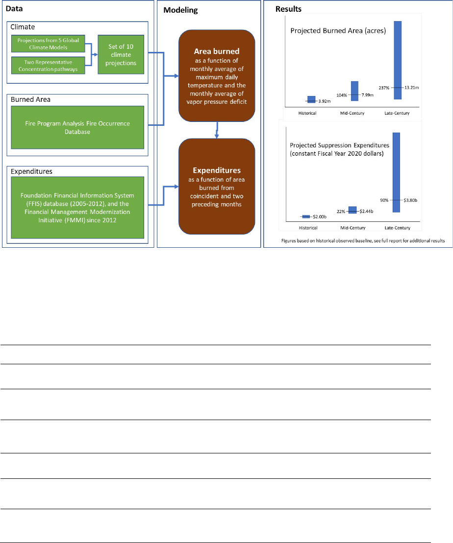
CLIMATE RISK EXPOSURE: AN ASSESSMENT OF THE FEDERAL GOVERNMENT’S FINANCIAL RISKS TO CLIMATE CHANGE
68
increases in area burned and inflation-adjusted suppression spending could plausibly double over
the next 80 years.
Figure A-1. Summary of area burned and suppression expenditure projections methods and
results across FS and DOI lands combined. Note: range and height of area burned and
suppression spending bars in the right panel reflect an 80% uncertainty bound.
Table A-1. Detailed projections of area burned and suppression spending, by DOI and FS and
combined.
Projected change in area burned by mid-century (fiscal years 2041-2059)
Compared to:
Forest Service
(FS)
Dept. of Interior
(DOI)
Combined FS &
DOI
Observed climate
94%
114%
104%
Modeled, climate back-cast
129%
83%
106%
Projected change in real suppression expenditures by mid-century (fiscal years 2041-2059)
Compared to:
Forest Service
(FS)
Dept. of Interior
(DOI)
Combined FS &
DOI
Observed climate
16%
57%
22%
Modeled, climate back-cast
109%
48%
83%
Projected change in area burned by late-century (fiscal years 2081-2099)

CLIMATE RISK EXPOSURE: AN ASSESSMENT OF THE FEDERAL GOVERNMENT’S FINANCIAL RISKS TO CLIMATE CHANGE
69
Compared to:
Forest Service
(FS)
Dept. of Interior
(DOI)
Combined FS &
DOI
Observed climate
244%
226%
237%
Modeled, climate back-cast
306%
180%
241%
Projected change in real suppression expenditures by late-century (fiscal years 2081-2099)
Compared to:
Forest Service
(FS)
Dept. of Interior
(DOI)
Combined FS &
DOI
Observed climate
85%
128%
90%
Modeled, climate back-cast
234%
114%
186%

CLIMATE RISK EXPOSURE: AN ASSESSMENT OF THE FEDERAL GOVERNMENT’S FINANCIAL RISKS TO CLIMATE CHANGE
70
Introduction
There is little doubt that changes in climate will affect wildlands, wildland fire, and suppression
of fire (Abatzoglou and Kolden 2013, Abt et al. 2009, Flannigan et al. 2005, Flannigan et al.
2006, Flannigan et al. 2016, Littell et al. 2009, Littell at al. 2016, Liu et al. 2014, McKenzie et al.
2016, Mitchell et al. 2014, Prestemon et al. 2009, Riley et al. 2019, Westerling et al. 2006).
Direct increases in area burned and numbers of large fires, resulting from more days with
extreme fire weather, longer periods of sequential days with extreme fire weather, and longer fire
seasons in many parts of the world are to be expected (Abatzoglou et al. 2021, Gao et al. 2021,
Jolly et al. 2015, Lenihan et al. 2003, Riley and Loehman 2016). Natural ignition patterns may
change with shifting storm tracks and lightning occurrence (Romps et al. 2014), and there are
likely to be changes in human ignition patterns due to land use change. Using an approach
similar to that used in Hope et al. (2016), this analysis evaluates an aggregate set of data on US
Federal wildfire area burned and Federal suppression expenditures and projects both area burned
and expenditures to calculate the effect of climate on Federal area burned and Federal
expenditures in mid-century (2041-2059) and late-century (2081-2099). We evaluate area burned
and wildfire suppression expenditures for both the USDA Forest Service (FS) and the US
Department of the Interior (DOI). The FS and DOI were modeled separately because their
management objectives differ, as did data availability.
Methods
Overview
This study extends similar work done in 2016 (Executive Office of the President 2016, USDA
Forest Service 2016). In the 2016 study, we used the two-step model approach where area
burned was projected and then projected area burned was used in a model of suppression
expenditures. We take this two-step approach in the 2021 study also. However, we refined the
models in terms of variables and time period and expanded the number of climate projections
used. For this analysis, we were able to obtain data and project suppression expenditures for
Alaska. For model fitting on wildfire to climate variables for the continental United States
(CONUS), we assembled monthly data from fiscal year 1993 to fiscal year 2019 for the Forest
Service and fiscal year 1993 to fiscal year 2018 for the Department of the Interior.
In the present study, the final burned area models, specified by region of the continental United
States (CONUS), were Poisson pseudo-maximum likelihood (PPML) models with variables of
monthly maximum temperature and vapor pressure deficit (e.g., Motta 2019).
52
This
combination of variables for projected area burned performed better out of sample (random and
52
The assumption of a constant mean/variance proportion restriction of the PPML model could have been relaxed with
estimation of other functional forms. See the Variable Preselection and Model for Area Burned section for additional explanation
of the choice of the PPML model.

CLIMATE RISK EXPOSURE: AN ASSESSMENT OF THE FEDERAL GOVERNMENT’S FINANCIAL RISKS TO CLIMATE CHANGE
71
end of series hold-out) than alternatives (linear, log-transformed area burned). Log-
transformation of maximum temperature (in degrees Kelvin) and VPD in the PPML
specifications slightly improved the out-of-sample goodness-of-fit (as measured by root mean
squared error and bias) of the area burned projections compared to leaving temperature and VPD
untransformed. Each CONUS region of the Forest Service and each corresponding collection of
lands managed by the Department of the Interior defined by the boundaries of each CONUS
Forest Service region, was allowed to differ in its relationship of area burned to climate
variables.
For model fitting on suppression expenditures, we had consistent monthly data for each region of
the Forest Service from 2005-2020. For DOI, suppression expenditures were available only in
aggregate across the entire agency, 2013-2020. We considered evaluating suppression spending
using preparedness levels, but the preparedness level (PL) time series was short, and the use of
PL’s would have required development of a new method to project them to 2100, which was
beyond the scope of this study.
Variable Preselection and Model Formulation for Expenditures
We initially tested linear models of suppression expenditure as a function of area burned to test
for model feasibility, and we found that these models performed well, particularly when
compared with univariate time series models (i.e., modeling spending as a function of lags of
spending and seasonal components). For the Forest Service, we considered fixed-effects three-
staged-least squares models of area burned, an approach used in the 2016 effort, but opted to
exploit the greater frequency of expenditure data (as monthly) and specify expenditures
separately for each of FS regions 1-9 with two-stage least squares (2SLS) methods, with
expenditures in the region as a function of instrumented current month area burned in the region
and the two most recent months’ lags of area burned in the region. Instruments current month
area burned were the current number of fires reported and the current month natural log of
human population of counties (U.S. Census Bureau 2021) containing national forests in the
region. For Forest Service Region 10 (Alaska), expenditures were statistically unrelated to area
burned and, given that they have been historically relatively low compared to the agency overall,
averaging $1.4m/year, 2005-2020, they were modeled as a function of a constant only. For the
Rest of the Forest Service (covering national contracts, the Washington, DC, office, and research
stations), expenditures were also modeled as a function of the current month area burned on all
national forests in regions 1-9, with current area burned instrumented by the total number of
wildfires on national forests in regions 1-9 and the natural log of the sum of the population of
counties containing national forest lands across each of the Forest Service regions 1-9. Because
Department of the Interior expenditures were not available for physical regions like the Forest
Service, total nationwide DOI expenditures, also reported monthly, were modeled with 2SLS
methods, with expenditures specified as a function of current month area burned (instrumented

CLIMATE RISK EXPOSURE: AN ASSESSMENT OF THE FEDERAL GOVERNMENT’S FINANCIAL RISKS TO CLIMATE CHANGE
72
with the number of wildfires on DOI lands across all of CONUS and the natural log of
population in counties containing DOI lands in CONUS—i.e., excluding Alaska and Hawaii).
Because stationarity is required for regressors in the models described above, we also carried out
several tests (augmented Dickey-Fuller, DFGLS, Phillips-Perron) of stationarity of the time
series of real dollar monthly expenditures at the regional level for the Forest Service and the
national level for DOI. All Phillips-Perron stationarity tests rejected a unit root at stronger than
1% for all Forest Service regions, Rest of Forest Service, and for the aggregate of DOI
expenditures. Dickey-Fuller generalized least squares tests rejected stationarity for FS regions 1,
2, 8, 9, 10, and RFS when specifying lagged difference terms using the Schwarz Information
Criterion but less commonly under other optimization criteria. We therefore evaluated the
existence of long-term stable relationships (cointegrating relations) between RFS spending and
CONUS area burned on Forest Service lands, and between DOI spending and CONUS area
burned on DOI lands with a Johansen cointegration rank test for these two series. Rank tests
could not reject nulls of no cointegration. Given the non-confirmatory test outcomes on
cointegration, as a further examination of the possibility that expenditures were nonstationary,
expenditures for RFS and DOI in aggregate were each modeled in first-differences, regressed on
the first-differences of current and two months’ lags of CONUS area burned. Tests with a small
number of Monte Carlo iterations with those specifications produced unstable long-term
projections (to late-century), with increasing variance and even negative expenditures projected
for DOI. We therefore retained models of expenditures in levels as a function of area burned in
levels for the projections reported here.
With monthly data on expenditures, it is natural to consider the existence of seasonal effects in
spending that need to be accounted for. However, for the expenditures of the Forest Service and
DOI, in nearly every case in every region, seasonality—measured with month indicator (dummy)
variables—was found to be not statistically significant, after controlling for area burned.
Therefore, we ignored potential seasonality in our expenditure models.
Finally, given the possibility of serial correlation in spending, we tested for residual serial
correlation in the second stage equations of our suppression expenditure models. Durbin-Watson
tests on the residuals confirmed nonsignificant serial correlation.
Variable Preselection and Model Formulation for Area Burned
Given accepted research, it has been shown that area burned in the United States can be
adequately and accurately modeled as a function of temperature, moisture, and a variety of
indices that derive from those two variables that determine flammability and rate of spread of
wildfire. We tested a suite of climate variables that have been projected into the future by the
Global Climate Models, downscaled using the Multivariate Adaptive Constructed Analogs
(MACA) process (Abatzoglou 2013, Abatzoglou and Brown 2012). These climate variables
included monthly average of daily maximum temperature, monthly total of daily precipitation,
monthly average of vapor pressure deficit (VPD) and monthly total potential evapotranspiration
CLIMATE RISK EXPOSURE: AN ASSESSMENT OF THE FEDERAL GOVERNMENT’S FINANCIAL RISKS TO CLIMATE CHANGE
73
(PET). In the 2016 study, the single climate variable selected for inclusion in the 2016 model
was the fiscal year annual average of daily maximum temperature. However, with the longer
historical timeline, we chose to use monthly, regional observations as the basis for the area
burned models for each agency. We tested the strength of the relationship between area burned
and other climate variables in addition to temperature. Temperature has been shown to influence
fuel moistures, fire season length, extreme fire weather, and lightning and storm tracks—all
conditions that are known to influence area burned (Flannigan et al. 2009, Flannigan et al. 2016,
McKenzie et al. 2004, Mueller et al. 2020, Romps et al. 2014, Wang et al. 2016). Abatzoglou
and Kolden (2013) state that area burned is influenced by temperature, precipitation, and drought
but contend that using temperature is merely a proxy for the many ways climate can influence
wildfire. Precipitation has also been shown to have a strong link with area burned, particularly
when standardized to percentile across an observed period (Abatzoglou and Kolden 2013,
Holden et al. 2018, Keeley and Syphard 2017, Mueller et al. 2020, Riley et al. 2013). While we
did test total monthly precipitation, we chose not to test the percentile of precipitation; finding a
way to combine historical and projected data to provide reasonable percentile precipitation
estimates by region and month may prove fruitful but was not completed in this study due to
time constraints. Vapor pressure deficit (VPD) is a metric incorporating both temperature and
relative humidity. VPD indicates how much moisture is in the air relative to the maximum
amount of moisture that the air could hold. VPD has also been shown to correlate strongly with
large fire events and area burned (Mueller et al. 2020, Seager et al. 2015, Williams et al. 2019).
PET was included as a candidate variable because area burned has been found to correlate with
drought (Abatzoglou and Kolden 2013, Lammon et al. 2014, McKenzie et al. 2017, Riley et al.
2013). We had initially hoped to include Energy Release Component (ERC) as a candidate
variable due to its high documented correlation with area burned (Riley et al. 2013, Riley and
Loehman 2016), but the computational time required for obtaining forecasts of ERC at spatial
and temporal scales suitable for our analysis were beyond the study timeframe.
Research on human-caused fires indicates that local population and income can influence
ignitions (Mercer and Prestemon 2005, Prestemon et al. 2013) and area burned (Prestemon et al.
2016). In addition, anecdotal evidence implies that as population increases, buildings and other
structures increase, which diverts suppression efforts from land protection to point protection.
This, too, could lead to increases in area burned, all else held constant. Increases in income are
hypothesized to influence the extent of local power and influence, which has been shown to lead
to increased suppression expenditures (Donovan et al. 2011). Such effects have been identified at
small spatial scales, at the level of the county or smaller. However, less research exists on such
relationships at such large spatial scales as whole collections of national forests (e.g., FS
regions). Testing of area burned models that included population in the counties containing
national forests or DOI lands revealed no significant effects. We estimated Poisson pseudo-
maximum likelihood (PPML) models of regional area burned as a function of the level and first-
CLIMATE RISK EXPOSURE: AN ASSESSMENT OF THE FEDERAL GOVERNMENT’S FINANCIAL RISKS TO CLIMATE CHANGE
74
difference of regional human population. Significances were uncommon across the 8 physical FS
regions and 8 physical DOI regions and signs on parameter estimates were not consistent.
Absence of evidence does not provide evidence of absence: population estimates in counties
contain errors, and changes between months within the short time series of years therefore are
unlikely to provide accurate information on the effects of humans on spending at the scale of the
region. We concluded that the area burned in an entire region and the population in the counties
of that region may not have been as spatially connected as would be required to identify
significant effects of population on wildfire (and its spending).
Modeling of area burned should address the zero bound on area burned. One way to recognize
this is through either log-transformation of area burned (assuming no months with zero area
burned, in our case) or the application of models such as the Tobit or pseudo-Poisson maximum
likelihood specifications. We evaluated linear models (which ignored zero-truncation) and
PPML models under out-of-sample forecasting conditions over historical data. We found that
PPML models out-performed linear models and avoided the possibility that projected area
burned would be negative. We did not test all alternative functional forms that would recognize
zero-truncation of the dependent variable (area burned). However, we tested the fit of a Negative
binomial maximum likelihood (NBML) model. The NBML model had a slightly better fit out-of-
sample, but random samples drawn during Monte Carlo simulation using that functional form
sometimes did not allow for convergence of the likelihood function, making the method less
reliable for simulations. Therefore, we opted to model area burned as using PPML models, as a
function of monthly maximum daily temperature in degrees Kelvin, transformed by the natural
logarithm, and monthly average vapor pressure deficit, also log-transformed. Exceptions to the
two variable specifications were made for FS regions 3 and 5, where maximum temperature was
dropped, and DOI regions 4, 5, and 6, where VPD was dropped.
The models we selected projected area burned as a function of the monthly average of maximum
daily temperature and the monthly average of vapor pressure deficit (VPD). This combination of
variables for projected area burned, although very highly correlated in the historical time series (r
> 0.92 in all regions evaluated), performed better out of sample (random and end of series hold-
out). Log-transformation of maximum temperature (in degrees Kelvin) and VPD (in kPa) slightly
improved the out-of-sample fitness of the area burned projections. Modeling area burned
requires some strong assumptions, that, in the face of a changing climate, could be difficult to
justify. We expect climate change to alter forest and range ecosystem compositions, and
vegetation changes will, in turn, alter how many acres burn and how often and intensely they
burn. In this analysis, because hazardous fuels are not directly modeled, our models carry an
assumption that these vegetation changes will not matter to either area burned, nor to the
expenditures we make to suppress wildfire. It is possible that, to the extent these changes have
already begun to occur across Federal wildlands, our models incorporate some of these changes
in ecosystems, but we cannot test this possibility using an aggregate model structure alone.

CLIMATE RISK EXPOSURE: AN ASSESSMENT OF THE FEDERAL GOVERNMENT’S FINANCIAL RISKS TO CLIMATE CHANGE
75
Likewise, our projections assume that parametric relationships only account for the effects of
wildland hazardous fuels management efforts that have been taking place in the historical time
period. Because we do not include variables directly indexing such management, no what-if
scenarios were carried out that would evaluate how Federal efforts to accelerate rates of
hazardous fuel reduction would affect wildfire and suppression spending. Detailed vegetation
modeling would be required to determine the extent to which climate-induced and management
caused changes in hazardous fuels would occur and therefore have effects on wildfire and
suppression expenditures.
Data
Temporal and geographic extent: The expenditure data are monthly, based on the Federal fiscal
year (October 1 to September 30). We divided the United States into regions that coincide with
the USFS regions and roughly with the Geographic Area Coordination Centers of the National
Interagency Fire Center. Climate data is monthly also and is aggregated to these regions based on
Federal lands only. Socioeconomic data is aggregated to regions based only on counties which
include Federal lands. Fire data, also monthly, is based on actual fire ignition locations from the
FPA FOD (fiscal years 1993-2018) (Short 2021). Monthly expenditure data for DOI are
available nationally, while consistent monthly data for the FS are available nationally for fiscal
years 2005-2020 by Forest Service Region, whose regional boundaries closely match GACC
boundaries. Given the varying starting and end-dates of wildfire and suppression data, model
data used in this study were truncated at the end of fiscal year 2018.
We used the Forest Service’s 2020 Resources Planning Act Assessment (RPA) climate
projections, which comprise 5 climate models projecting under the Representative Concentration
Pathways (RCPs) RCP 4.5 and RCP 8.5 scenarios (Langner et al. 2020). The RPA climate data
set is a subset of the MACAv2METDATA set (Abatzoglou and Brown 2012, Abatzoglou 2013).
Global climate historical modeled projections (1950-2005) and future projections (2006-2099)
from the Coupled Model Inter-Comparison Project 5 (CMIP5) were downscaled to the 4-km grid
size using the Multivariate Adaptive Constructed Analogs (MACA) method. The MACA method
is a statistical downscaling method that uses historical observations to remove historical biases
and match spatial patterns in climate model output.
The RPA data set contains the historical data (METDATA, 1979-2015), and the historical
modeled data (1950-2005) and the future projections (2006-2099) (MACAv2-METDATA) for 5
climate models under two Representative Concentration Pathways (RCP 4.5, 8.5) (Table B1).
Five climate models were selected to capture the future (2041-2059) range of the 20-model
MACAv2-METDATA set (Langner et al. 2020). Rather than use an ensemble, a model that
projected future change near the mean of all 20 projections was selected: NorESM1-M. The five
models reflect the hottest projection (HadGEM2-ES365), the least warm projection (MRI-
CGCM3), the wettest projection (CNRM-CM5), the driest projection (IPSL-CM5A-MR), and
the middle of the range projection (NorESM1-M) (see

CLIMATE RISK EXPOSURE: AN ASSESSMENT OF THE FEDERAL GOVERNMENT’S FINANCIAL RISKS TO CLIMATE CHANGE
76
http://maca.northwestknowledge.net/GCMs.php for detailed descriptions of these models). The
data set and metadata are available at:
Historical: https://www.fs.usda.gov/rds/archive/catalog/RDS-2017-0070-2
Projections: https://www.fs.usda.gov/rds/archive/catalog/RDS-2018-0014
For this project, we added monthly vapor pressure deficit from MACAv2METDATA to the RPA
historical and projected climate data sets. We also added four years’ worth of monthly data to all
variables in the RPA historical data set (2016-2019) from GRIDMET, which is the data set from
which the RPA historical data were derived (Abatzoglou 2013).
We generated regional and national averages, monthly and annual, for maximum daily
temperature, average VPD, total PET, minimum daily relative humidity, and the sum of daily
precipitation. We created regional monthly averages by first converting all daily or monthly
spatial data to Albers Equal Area Conic to ensure grid cells from differing datasets matched, and
included only grid cells corresponding to Federal lands (USDA Forest Service or DOI) (Snyder
1987).
Most of the global climate models available in the MACAv2 data set have been evaluated for
their performance relative to historical climate observations. Based on the analysis by Sheffield
et al. (2013), at the conterminous US scale, the models that had the least bias in temperature
included MRI-CGCM3, used in this study. For precipitation, the models with the least bias
included CNRM-CM5 and NorESM1-M, used here. At the regional scale, the models that
performed best included IPSL-CM5A-LR, used in this analysis. Simulations of the 20
th
century
by CMIP5 models have been conducted for regions of the United States: Pacific Northwest
(Rupp et al. 2013), Southeast (Rupp 2016), and for the Southwest (Rupp Pers. Comm.). Based on
these regional analyses, the top five models, based on 18 metrics, included CNRM-CM5 and
HadGEM2-ES, used in this analysis.
Figure B-1 shows the historical and projected maximum temperature and vapor pressure deficit
area-weighted for nationwide by agency for the observed period and all modeled periods. The
values of each variable during each time period differ by agency, but there are some trends to
note. First, for both variables, values are higher for DOI lands than for Forest Service lands in the
observed and backcast data, and that remains the case in the future periods. Second, for each
agency, the median values across the ten futures for both variables are greater in the two future
periods than for the backcast and observed periods, indicating increasingly hotter temperature
extremes, and drier conditions expected on average. Compared with backcast values, maximum
monthly temperatures for both DOI and Forest Service lands are expected to increase by nearly 2
degrees by mid-century and more than 3 degrees by late century on average across the 10
futures, with the greatest increases projected under the hottest (HadGEM2-ES365) and driest
(IPSL-CM5A-MR) projections under RCP 8.5 for both agencies. Average projections of VPD
for the U.S. across the ten futures show expected increases by 0.1 kPa at mid-century and 0.2
CLIMATE RISK EXPOSURE: AN ASSESSMENT OF THE FEDERAL GOVERNMENT’S FINANCIAL RISKS TO CLIMATE CHANGE
77
kPa at late century for Forest Service lands, and by 0.2 and 0.3 for DOI lands for the two time
periods, respectively. In all cases for both variables and both agencies, the range in average
values across the ten futures for the U.S. is greater at late century than for mid-century,
corresponding with increasing uncertainty in the climate model projections over time. While the
projected values for both variables differ by region, there are consistent trends by region
(Appendix Figures B-1 and B-2). Increases in both maximum temperature and VPD are also
expected for each region at mid-century and late century. Average projected maximum
temperature was greatest in the Southern region for both agencies at mid-century and late
century, while the greatest increases in maximum temperature were projected in the Eastern
region. For VPD, on average across the ten futures, the greatest values were projected for Forest
Service lands in the Southwestern region and for DOI lands in the Pacific Southwest, while the
greatest increases were projected for both agencies’ lands in the Southwestern region.
Area burned (in acres) and number of fires were provided by Karen Short from the Fire Program
Analysis Fire Occurrence Database (Short 2021). This dataset includes point locations, discovery
dates, and final area burned estimates from individual agency fire reports estimates that were
aggregated by month and jurisdictional agency for FY1993 to 2018. Additional FS data for FY19
were obtained from FIRESTAT, as noted above. We were unable to acquire and properly
compile additional FY19 data from DOI due to time constraints. We used area burned for
CONUS (excluding Alaska) for both FS and DOI expenditure modeling, although we also
projected Alaska spending for the Forest Service separately without making projections of area
burned. Although spending in Alaska (Region 10) for the Forest Service is low, averaging less
than $1m/year, wildfire area burned on DOI lands in Alaska are more significant. Alaska
represents a significant acreage in many years (averaging 37%, 1993-2018, but ranging from 3%
to 93% of total DOI area burned), but a much smaller expenditure (we only have five years of
expenditure data by region, but the average is 8%, and the range is from 4-14% of total DOI
expenditures). With this level of variability, and a clear disconnect between area burned and
expenditures, along with inadequate data for modeling Alaska expenditures separately, we chose
to not model area burned in Alaska and used projected CONUS area burned as the dependent
variable in projecting total nationwide expenditures for both DOI and expenditures only for non-
region spending for the category Rest of Forest Service. For Forest Service regions, 1-9,
however, we model expenditures as a function of each region’s area burned. For Forest Service
Region 10 (Alaska), we model it as simply a constant.
Suppression expenditure data: All expenditures are in constant 2020 dollars (obtained from the
President’s Budget, “Table 10.1—Gross Domestic Product and Deflators Used in the Historical
Tables: 1940-2026”, at https://www.whitehouse.gov/omb/historical-tables/). Regional
expenditure and RFS expenditure data for the Forest Service were monthly, 2005-2020. For the
Department of the Interior, data were also monthly, 2013-2020. The national level data are from
NIFC, and the FS regional data are derived from historical reports, the Foundation Financial

CLIMATE RISK EXPOSURE: AN ASSESSMENT OF THE FEDERAL GOVERNMENT’S FINANCIAL RISKS TO CLIMATE CHANGE
78
Information System (FFIS) database (2005-2012), and the Financial Management Modernization
Initiative (FMMI) since 2012.
Projections
To generate a no-further-climate change average for area burned and expenditures for 2006-2018
for FS and DOI, we averaged the historical data. In addition, we produced a median of the
backcast of the regression models using historical modeled climate variables. The projections for
midcentury represent an average of 2041-2059, and late-century are an average of 2081-2099
(the year 2100 is not included in the MACA dataset).
We used the projected climate data in our selected models to generate future area burned for
midcentury and late-century, and then used area burned in the expenditure projections. We also
calculated a change in area burned from recent to the two future periods. There are two possible
methods of projecting with the climate values from the GCMs: (1) use the historical observed
data as the base and use the projected climate data to estimate the change, or (2) use the climate
model backcast projection as the base and the projected data as the change. We report both in
this document.
The Monte Carlo simulations involved (1) randomly sampling from monthly observations of area
burned and backcast historical climate over fiscal years 2006-2018, monthly observations of FS
suppression expenditures over fiscal years 2006-2018, and monthly observations of DOI
suppression expenditures over fiscal years 2013-2018; (2) estimating statistical relationships for
area burned and suppression spending with the randomly sampled data; (3) projecting area
burned and spending through fiscal year 2099 with the estimated parameters; and (4) repeating
steps (1)-(3) 500 times for each of the climate projections (each of the 10 GCM x RCP
combinations). Monte Carlo projection results are summarized in terms of medians of area
burned and expenditures, 80% and 90% upper and lower bounds of area burned and
expenditures, and then medians across each of the 10 climate projections. We generated
projected expenditures and area burned for each of the climate models. Results were also
summarized in tabular form, reporting historical observed, historical modeled (fiscal years 2006-
2018) for area burned and expenditures for the Forest Service and DOI and their total, including
80% and 90% upper and lower bounds and medians for mid-century and late-century.
Results
Area burned modeling results
Area burned model estimates are reported in Table B-1. Models indicate good fit and high
significance of both maximum temperature and VPD. Constant terms are also significant in most
cases. Pseudo-R
2
’s indicate that a sizeable portion of historical variation is explained by the data
in most regions for both agencies. Generally, VPD is positively related to area burned. In cases
when maximum temperature is included as an additional predictor, maximum temperature is

CLIMATE RISK EXPOSURE: AN ASSESSMENT OF THE FEDERAL GOVERNMENT’S FINANCIAL RISKS TO CLIMATE CHANGE
79
negatively signed. In cases when VPD is not present (DOI regions 4, 5, and 6), maximum
temperature is positively signed. Because maximum temperature is positively correlated with
VPD, the latter set of results is expected. For any given value of VPD, a lower temperature
means that relative humidity is lower, and thus fires would be expected to burn hotter.
Expenditure modeling results
Expenditure equation estimates are reported in Table B-2. Models indicate that current month
area burned and two lags of area burned are usually significant for each region or aggregate
modeled. Because the two lags were not significant in initial estimates of the Rest of Forest
Service model, those lags were dropped for reporting and for models used in Monte Carlo
projections.
Projections
Area Burned Projections
Area burned projections for the FS and DOI in aggregate are shown in Figures B-2 through B-4.
(Regional detail of median area burned across all climate projections is presented in Appendix
figures C-3 through C-6.) In the left panel of each of these figures is reported the median and the
upper and lower bounds of an 80% confidence band for the total of FS plus DOI (48-state
CONUS). The confidence bands only account for parameter uncertainty in the regional area
burned models across the ten climate projections. In the right panel in each is the median for
each of the ten climate projections. Figure B-2 is for total (FS + DOI), Figure B-3 is FS only, and
Figure B-4 is DOI only. In all figures, it is apparent that late-century area burned varies widely
across projections, with the highest area burned projected by the HadGEM2-ES365 (hot) climate
model under the RCP 8.5 scenario. The lowest area burned projections emerged from the least-
warm model, MRI-CGCM3 under the RCP 4.5 scenario. The figures demonstrate clearly how
late-century area burned varies widely across climate projections, a result that might have been
expected, given the wide variability across projections in late-century maximum temperature and
VPD (Figure B-1).
Tables B-3 through B-5 report the Monte Carlo area burned projections numerically. Tables are
organized to show observed area burned over our benchmark years of 2006-2018, model
projections of area burned over the benchmark years using backcast climate data from each of
the GCM x RCP projections, and then projections of median area burned in mid-century (2041-
2059) and late-century (2081-2099). The “All Scenario Median” and the 80% and 90% upper
and lower confidence bounds reported are based on the combined 10 climate projections x 500
iterations/projection = 5,000 total iterations.

CLIMATE RISK EXPOSURE: AN ASSESSMENT OF THE FEDERAL GOVERNMENT’S FINANCIAL RISKS TO CLIMATE CHANGE
80
Table B-3 shows the total of area burned for the FS and DOI. Broadly, the table shows general
agreement between observed area burned for CONUS (3.92 million acres/year, 2006-2018) and
backcast area burned for the same period (medians of the 10 climate projections range from 3.20-
4.91 million acres/year). By mid-century, when compared to observed historical area burned,
area burned in aggregate for FS + DOI is projected to be 21% to 251% higher and by late-
century 35% to 1929% higher. Compared to backcast historical climate, these percentages range
from 22% to 201% higher in mid-century and 65% to 1641% higher in late-century. The medians
across all climate projections are 104% and 237% by mid- and late-century compared to
observed historical and 106% and 241% compared to modeled historical area burned.
Table B-4 reports the results for just the FS CONUS lands. Variability is similar to that shown in
Table B-3. Just as for the FS + DOI in aggregate, there is wide variation across the ten climate
projections. Across all ten climates for the FS, median area burned is 94% and 244% higher by
mid- and late-century, respectively, compared to observed historical area burned, and 129% and
306% higher by mid- and late-century when compared to modeled historical area burned.
Table B-5 shows the same results but for DOI lands in CONUS. Here again, there is wide
variation across the ten climate projections and demonstrates the same trends as reported for FS
lands in CONUS. Compared to observed historical (2006-2018) area burned in CONUS, DOI
median area burned in CONUS is projected to be 114% and 226% higher by mid- and late-
century, respectively. Compared to modeled historical, median area burned is projected to be
83% and 180% higher in mid- and late-century, respectively.
It is notable that the median values for area burned, 2006-2018, using backcast climate
(maximum temperature, VPD) variables (second column of values in tables B3 through B5)
reveal possible statistical biases produced by each of the climate projections (GCM x RCP
scenario). Combined FS + DOI (Table B-3) has little overall bias when measured by the “all
projections median” value (3.88 million acres/year) versus the observed value (3.92 million
acres/year). For the Forest Service, however, the backcast projections tend to under-predict in the
2006-2018 benchmark period (1.51 million acres/year backcast versus 1.79 million acres/year
observed), while the opposite is shown for DOI (2.33 million acres/year backcast versus 2.00
million acres/year observed). Because no climate projection can perfectly predict the backcast
values of all climate variables, the lack of perfect alignment of median backcast predictions with
the historical area burned is not unexpected, although particular GCMs tend to predict lower and
others higher than the observed area burned. For example, the “least warm” model (at RCP 4.5
and 8.5) predicts the lowest, while the “dry” and “hot” models (at 4.5 and 8.5) predict the highest
in the 2006-2018 backcast for both FS and DOI. Those tendencies to predict low or high might in
part explain the lower and upper ranges of projected area burned outcomes projected for mid-
and late-century shown in the tables.
Expenditure Projections
CLIMATE RISK EXPOSURE: AN ASSESSMENT OF THE FEDERAL GOVERNMENT’S FINANCIAL RISKS TO CLIMATE CHANGE
81
Graphs showing projections of expenditures are reported in figures B-4 through B-6. Just as for
area burned, each figure has a left panel showing the median and 80% upper and lower bound
projections of expenditures across all 10 climate projections, while the right panel in each shows
the median projections for each of the 10 climate projections. Clear in all cases is that the high
variability, particularly in late-century, in area burned is translated into high variability in
projected expenditures.
Data from the graphs are summarized in tables B-6 through B-8. Data in the tables are reported
in the same way as for area burned projections, enabling comparisons between annual totals of
area burned observed and projected in the benchmark historical period of 2006-2018. Like for
area burned, the “All Scenario Median” and the 80% and 90% upper and lower confidence
bounds reported are based on the combined 10 climate projections x 500 iterations/projection =
5,000 total iterations. As reported in Table B-6, in mid-century compared to observed historical,
median expenditures (in 2020 dollars) range from 24% lower to 121% higher, and for late-
century 16% lower to 1353% higher. Compared to modeled historical, they range from 26%
higher to 190% higher by mid-century and 42% to 1805% higher when compared to modeled
historical. In aggregate across FS + DOI, median projected real expenditures across all ten
climate projections are 22% and 90% higher by mid- and late-century, respectively. When
compared to projected expenditures, they are 83% and 186% higher for mid- and late-century,
respectively.
Tables B-7 and B-8 document how variability across projections in future expenditures is
connected closely to variability in area burned. Across all climate projections, FS (Table B-7)
median suppression spending is projected to be 16% higher and 85% higher in mid- and late-
century compared to observed historical and 109% and 234% higher when compared to modeled
historical. Comparable figures for DOI (Table B-8) are 57% and 128% higher in median
suppression spending by mid- and late-century, respectively, when compared to observed
historical and 48% and 114% higher when compared to modeled historical spending.
Discussion and Conclusions
The models developed here show that expenditures respond to changes in area burned as
expected, and that area burned increases with increasing vapor pressure deficit and, in some
cases, average maximum temperature. Area burned is projected to increase by double or triple-
digit percentages across most of the ten projections we evaluated. Real dollar suppression
expenditures are projected to increase by similarly large percentages.
While vapor pressure deficit and temperature are only two of several climate measures that have
been linked to wildfire area burned, we found that unbiased backcasts of area burned and
expenditures could be obtained from parameterizing these simple relationships. However, model

CLIMATE RISK EXPOSURE: AN ASSESSMENT OF THE FEDERAL GOVERNMENT’S FINANCIAL RISKS TO CLIMATE CHANGE
82
simplicity likely trades off with higher uncertainty in making projections, so definitive
conclusions about the long-run status of wildfire and associated suppression on Federal lands in
the United States may not be warranted without acknowledgment of these uncertainties. In the
following section, we detail several reasons why uncertainty is large when envisioning the
evolution of wildfire and expenditures.
Wildfire area burned and suppression spending display high uncertainty in their projected
futures, particularly by late-century. We note that actual FS spending (and total FS + DOI
spending) since 2015 has exceeded even the 80% uncertainty upper bound modeled in this
report, hinting that structural changes might be underway that will lead to spending that remains
well above projected median levels indefinitely. Additional modeling, perhaps directed at finer
spatial scales and accounting more directly for hazardous fuels, could reduce uncertainties and
help to reduce biases in model predictions. Nevertheless, it is possible that, even with improved
models based on historical data, there will be structural changes in how fires burn under novel
climates and novel vegetation assemblages, how fire managers apply suppression resources
under shifting wildfire regimes, and in the unit costs of suppression resources over time. Such
changes would imply that the projections reported here provide progressively less useful
guidance, moving from mid- to late-century.
Caveats and Assumptions
Our models involve a number of assumptions, violation of any of which would alter both the
projected changes in spending and the ranges of our confidence bands. These assumptions,
loosely grouped into aggregation bias (over space and time), omitted variable bias (including
climate, fire and socioeconomic variables) and modeling limitations, are discussed in more detail
below. Even with these caveats and assumptions, however, our models, along with the literature
we have cited (and much that we have not) provide evidence that both wildfire extent and
suppression expenditures are expected to increase with climate change. Our models, specifically,
show that vapor pressure deficit and/or temperature can account for significant increases in area
burned and that expenditures increase with increases in area burned.
Aggregation
The statistical models of area burned and of suppression spending are estimated using data
aggregated to regions and nationwide. Such aggregation, in the presence of heterogeneity in area
burned and spending processes, would bias parameter estimates in unknown directions.
Aggregation across space and time can interact with biases associated with omitted variables
(next caveat), resulting in findings of insignificance when in fact significant effects exist (i.e., it
can raise statistical Type II error rates). For both the FS and the DOI models of area burned, the

CLIMATE RISK EXPOSURE: AN ASSESSMENT OF THE FEDERAL GOVERNMENT’S FINANCIAL RISKS TO CLIMATE CHANGE
83
fact that each region’s area burn function was estimated separately allowed for the relationship
between wildfire and climate to differ across regions. Even so, the assumption involved for the
reported models is that fine-scale (finer than region level) wildfire area burned responds
identically to climate variables within that region. The FS models of the relationship between
suppression spending area burned were also allowed to vary across regions, but they still forced
the spending-burn relationship (i.e., real dollars per acre) to be constant within each region. For
the Department of the Interior, because total departmental spending was modeled as a function of
total area burned, the spending relationship to area burned implied constant spending per acre. A
similar forcing assumption was implied by non-regional spending of the Forest Service.
Omitted variables
Our statistical models of area burned and expenditures are parsimonious, with area burned
specified as a function of monthly maximum daily temperature and/or vapor pressure deficit.
There is little doubt that potentially influential variables are omitted in our chosen specifications.
Thus, these models assume that any omitted variables are orthogonal to the included variables, so
that errors in projections are contained in error terms that are unrelated to the included variables.
Alternatively, it could be that the omitted variables are perfectly correlated with the included
variables, in which case parameter estimates for included variables completely contain the
effects of the perfectly correlated omitted variables, and no bias would exist in resulting
projections.
One key factor potentially missing from the suppression spending models is direct attention to
human populations, which can lead to higher demands to protect property at the expense of area
burned and which can affect the distributions of aggregate wildland fuels. In addition, a specific
kind of omitted variables bias would emerge if past wildfires are negatively related to future
wildfires in the same locations, then wildfire area burned modeled without attention to this
process would be biased upward compared to reality. Although we tested for the relationship
between spending and human population levels and changes and found inconsistent and usually
non-significant effects, it is still possible that finer scale modeling of area burned could reveal
robust effects.
Recent research has concluded both that temperature is a reasonable measure of climate change,
but also that temperature is an insufficient measure of climate change influences on wildfire. In a
statistical analysis of the relationship between meteorological variables and area burned in
Canada, Flannigan and Harrington (1988) found that long sequences of days without rain, low
relative humidity, and maximum temperatures were the best predictors of area burned, while
rainfall and number of dry days per month were not significant. Romps et al. (2014) evaluated
the impacts of climate change on lightning and found that (a) the precipitation projections do not
show overall increases that would lead to increased lightning, and (b) increased temperature is
the major controlling factor leading to increased lightning projections. Temperature has been
CLIMATE RISK EXPOSURE: AN ASSESSMENT OF THE FEDERAL GOVERNMENT’S FINANCIAL RISKS TO CLIMATE CHANGE
84
shown to lead to a need for additional precipitation to hold fuel moistures constant (Flannigan et
al. 2016). This results from the changes in amount of water the air can hold at higher
temperatures—as temperatures increase the air can hold more water, which leads to drying of
fuels, even if precipitation stays the same. Flannigan et al. (2016) also conclude that increasing
temperatures lead to an increased number of extreme fire weather days.
For these analyses, we relied on mapping the association between temperature and vapor
pressure deficit and area burned into the future. However, the association between temperature
and area burned has been demonstrated to be relatively weak in the absence of some form of a
dryness metric (Littell et al. 2009). It is reasonable to expect that temperature is only one, and
perhaps not the most important one, of the climate variables affecting wildfire. However, this is a
testable, and as yet untested, hypothesis in relation to projecting aggregate wildfire extent and
expenditures. We show here only that temperature and vapor pressure deficit are significant, in
the absence of other climate measures, in affecting area burned. The combination of VPD and
maximum daily temperature in our models increased the goodness-of-fit of our models out-of-
sample compared to inclusion of these and other combinations of variables and also when those
measures were excluded.
In our models, many variables found in other research to affect both wildfire and suppression
were assumed constant throughout the projections, when it is unlikely that constancy will be
maintained to the end of this century. Thus, each of these assumptions represents an omitted
variable. We assumed that wildfire suppression strategies and technology do not change, and so
we did not need to include variables representing that change. We assumed that suppression will
not become more or less effective at limiting wildfire. We assumed that wildland fuels
management rates remain unchanged, in relation to overall wildfire activity. Research shows that
management of aggregate fuels on landscapes can affect how wildfires burn, likely affecting
suppression productivity and hence area burned or other damages upon which suppression is
focused (Loudermilk et al. 2014, Mercer et al. 2005, 2007; Thompson et al. 2013). However,
Bessie and Johnson (1995) compared the composite influences of fuels and climate and
concluded that climate was the driving force in year over year changes in area burned.
Nevertheless, the lack of direct statistical accounting for the effects of climate or management
efforts to reduce hazardous fuels adds a degree of uncertainty to the projections that may not be
reflected in our projections. Furthermore, models assume that allocations of suppression efforts
across threatened people, property, and resources will be allocated in the same ways, in response
to wildfire, as they have in the past. Because historical data on suppression spending and area
burned reflect averages of policies to protect people, property, and resources, substantial changes
in the ratios of these variables threatened by wildfires in the future could affect spending in ways
not accounted for in our projections.
In this analysis, the general approach and structure of wildfire management was assumed
constant over time. However, consequences to wildfires and costs from climate changes are
CLIMATE RISK EXPOSURE: AN ASSESSMENT OF THE FEDERAL GOVERNMENT’S FINANCIAL RISKS TO CLIMATE CHANGE
85
outside the range of reliable futuring over long time frames, except that new climates will modify
human activities and probably require alternative management approaches. Even within the near
future (10 to 20 years) analyzed in the Quadrennial Fire Review (QFR)
(https://www.forestandrangelands.gov/QFR/documents/2014QFRFinalReport.pdf) there exists “a
strong possibility that today’s regional wildland fire management dynamics will shift as a result
of climate and environmental factors”. Furthermore, the QFR identified the potential for a shock-
type wildfire event to instigate a fundamental realignment of Federal land and fire management
functions that would clearly alter the relationship between area burned and management cost. It
is doubtful that biologists and foresters in 1900 could have predicted the magnitude of wildfire
sizes, behaviors, damages to human and natural resources, and costs experienced today let alone
the types of equipment and suppression responses that occur. Due to the increased uncertainty of
both natural and human consequences of future climate, future management cost projections
should be evaluated with caution.
We also assume constant socioeconomic variables, including prices, population, and income. If
the per-unit cost of labor, capital, and other purchased inputs into suppression production were to
rise at a rate higher than inflation, then suppression expenditures would tend to be higher,
possibly also leading to lower overall suppression effort and then to greater area burned.
Generally, wages and capital costs have not been rising faster than inflation in the last 20 years.
However, as the economy and overall wealth grows, these per-unit prices of these inputs might.
Our projections indicate that, under some climate projections, area burned would increase several
fold over historical rates. As the projected annual area burned increases, however, this means
that substantially more acres would need to reburn, or that wildfire would need to move into
areas that historically have not burned, in order for these fires to have adequate fuel. Thus, our
models would overestimate the projected area burned, at least in forested landscapes.
Conversely, in drier, range ecosystems, it is possible that increases in burning rates could lead to
the potential for more fire, as reburning rates are expected to be higher in these ecosystems. For
these ecosystems, our models would underestimate the projected area burned. It is not known at
what burning rate these limiting conditions would be reached in either forest or range
ecosystems. Hope et al. (2016) capped their Canadian area burned estimates assuming a 20-year
fire return interval, equivalent to burning 5% of the wildland each year. Our results suggest that
by late-century, an average of nearly 6 million FS acres per year could burn, or about 3% of all
FS land, and we felt we had little justification for, in the absence of a statistically modeled
relationship, artificially capping our area burned estimates. Additionally, because the United
States has wide variation across ecoregions in wildfire return intervals (Greenberg and Collins
2021), simple solutions such as artificial caps would possibly add more uncertainty to our
projections, not less. It is possible that such relationships can be estimated, which would be an
area worthy of additional study and modeling efforts.

CLIMATE RISK EXPOSURE: AN ASSESSMENT OF THE FEDERAL GOVERNMENT’S FINANCIAL RISKS TO CLIMATE CHANGE
86
Modeling
We assumed that the included information from climate projections was adequate to capture
uncertainty regarding the effects of temperature and vapor pressure deficit on area burned on
Federal lands. We assumed that these systems could be approximated by an exponential
relationship, with no significant biases or added uncertainty due to spatial autocorrelation and no
significant effects of our assumption of mean-variance proportionality. More fundamentally,
because our models could only be based on historical relationships among variables, we assume
that those relationships will endure to the end of the century. Our models make long-run
projections, without evaluating which factors that are typically assumed fixed might be variable
in the long-run, such as fire regimes, biomes, and suppression strategies. In addition, even at
aggregate scales, the highly-modified forest and grassland ecosystems of U.S. Federal lands may
not bear much relation to either natural ecosystems or to ecosystems expected in the distant
future under climate change (McKenzie and Littell 2016).
Any model is an abstraction, a simplification of reality. In this analysis, we used only five
climate models under each RCP scenario. Thus, we assumed that five global climate model
realizations of future climate under the increased radiative forcing of either 4.5W/m
2
or of
8.5W/m
2
were sufficient to capture uncertainty regarding the temperature and climate futures on
Federal lands. Undoubtedly, additional projections under each RCP would have narrowed the
variability in the future. However, these five climate models allow us to explore a hot versus a
warm future and a wet versus a dry future. The large end of century projections by the Hadley
model under RCP 8.5 portend hot temperatures and increased wildfire area burned. In contrast,
the Least Warm model (MRI-CGCM3) projects the least change in area burned. While our
Monte Carlo simulations address uncertainty in the estimated coefficients as well as uncertainty
reflected in the multiple GCM temperature projections, we did not incorporate any within-GCM
uncertainty. The assumption here is that the multiple models can proxy for uncertainty within the
GCMs.
Uncertainty in wildfire projection exists even at the incident level, over the timeframe of hours to
days, and is compounded when working at decadal or century-long scales (Riley and Thompson
2016). One reason for compounding uncertainty is that shifts in vegetation assemblies and even
biomes are likely during this timeframe due to climate change, meaning fire regimes will also
shift (Lenihan et al. 2003, Loehman et al. 2014). Take, for example, the changes in fuels and
vegetation documented since the turn of the 20
th
century (Loope and Gruell 1973, Gruell 1983,
Gruell 2001). By first removing Indian burning (Lewis 1973, Barrett 1980), and then attempting
to remove wildfires, European settlement altered vegetation composition and structure, insect
outbreaks, and wildfire behavior beyond recognition in just 100 years of relatively subtle climate
changes. Feedbacks between shifting vegetation assemblies, changing climate, and altered
ignition patterns will be complex and may produce no-analog states.
Caveat summary
CLIMATE RISK EXPOSURE: AN ASSESSMENT OF THE FEDERAL GOVERNMENT’S FINANCIAL RISKS TO CLIMATE CHANGE
87
Wildfire and fire management, including suppression, is a complex system where individual
factors interact in complex, non-linear, unpredictable ways. What happens in one component of
the system will cascade through the system altering other components, and these cascades are
multidirectional. Climate change is expected to influence ignition patterns, fire weather,
ecological community composition, local community development, and our willingness and
ability to manage wildfire. Each of these changes will reverberate through the system, adding
uncertainty about the future of wildfire and suppression spending that may not be adequately
captured by the simple statistical relationships that drive the results presented in this study.
CLIMATE RISK EXPOSURE: AN ASSESSMENT OF THE FEDERAL GOVERNMENT’S FINANCIAL RISKS TO CLIMATE CHANGE
88
Literature Cited
Abatzoglou JT. 2013. Development of gridded surface meteorological data for ecological
applications and modelling. International Journal of Climatology 33:121–131.
Doi:10.1002/joc.3413
Abatzoglou JT, Brown TJ. 2012. A Comparison of Statistical Downscaling Methods Suited for
Wildfire Applications, International Journal of Climatology 32(5):772–780.
Doi:10.1002/joc.2312
Abatzoglou JT, Kolden CA. 2013. Relationships between climate and macroscale area burned in
the western United States. International Journal of Wildland Fire 22:1003–1020.
http://dx.doi.org/10.1071/WF13019
Abatzoglou JT, Juang CS, Williams AP, Kolden CA, Westerling AL. 2021. Increasing
synchronous fire danger in forests of the western United States. Geophysical Research Letters
48(2):e2020GL091377. https://doi.org/10.1029/2020GL091377
Abt KL, Prestemon JP, Gebert KM. 2009. Wildfire suppression cost forecasts for the US Forest
Service. Journal of Forestry107(4):173-178.
Barrett SW. 1980. October. Indian fires in the pre-settlement forests of western Montana.
In Proceedings of the Fire History Workshop. USDA Forest Service, General Technical Report
RM-81, Fort Collins, Colorado (pp. 35-41).
Bessie WC, Johnson EA. 1995. The Relative Importance of Fuels and Weather on Fire Behavior
in Subalpine Forests. Ecology 76:747–762. Doi:10.2307/1939341
Donovan GH, Prestemon JP, Gebert K. 2011. The effect of newspaper coverage and political
pressure on wildfire suppression costs. Society and Natural Resources 24(8):685-698.
Executive Office of the President. 2016. Climate Change: The Fiscal Risks Facing the Federal
Government—A Preliminary Assessment (November 2016), 73 pages.
https://obamawhitehouse.archives.gov/sites/default/files/omb/reports/omb_climate_change_fiscal_risk_re
port.pdf
Flannigan MD, Amiro BD, Logan KA, Stocks BJ, Wotton BM. 2006. Forest Fires and Climate
Change in the 21ST Century. Mitigation and Adaptation Strategies for Global Change 11:847–
859. Doi: 10.1007/s11027-005-9020-7
Flannigan MD, Harrington JB. 1988. A study of the relation of meteorological variables to
monthly provincial area burned by wildfire in Canada (1953–80). Journal of Applied
Meteorology 27:441–452.
Flannigan MD, Krawchuk MA, De Groot W, Wotton BM, Gowman LM. 2009. Implications of
changing climate for global wildland fire. Int J Wildland Fire 18: 483–507. Doi:
10.1071/wf08187
CLIMATE RISK EXPOSURE: AN ASSESSMENT OF THE FEDERAL GOVERNMENT’S FINANCIAL RISKS TO CLIMATE CHANGE
89
Flannigan MD, Logan KA, Amiro BD, Skinner WR, Stocks BJ. 2005. Future Area Burned in
Canada. Clim Change 72: 1–16. Doi: 10.1007/s10584-005-5935-y
Flannigan MD, Wotton BM, Marshall GA, De Groot WJ, Johnston J, Jurko N, Cantin AS. 2016.
Fuel moisture sensitivity to temperature and precipitation: climate change implications. Climatic
Change 134: 59. Doi:10.1007/s10584-015-1521-0
Gao P, Terando AJ, Kupfer JA, Varner JM, Stambaugh MC, Lei TL, Hiers JK. 2021. Robust
projections of future fire probability for the conterminous United States. Science of the Total
Environment 789:147872. https://doi.org/10.1016/j.scitotenv.2021.147872
Greenberg CH, Collins B. 2021. Fire Ecology and Management: Past, Present, and Future of US
Forested Ecosystems. Springer. 502 pages. https://doi.org/10.1007/978-3-030-73267-7
Gruell GE. 1983. Fire and vegetative trends in the Northern Rockies: interpretations from 1871-
1982 photographs. Gen. Tech. Rep. INT-158. Ogden, UT: U.S. Department of Agriculture,
Forest Service, Intermountain Research Station. 117 p.
Gruell GE. 2001. Fire in Sierra Nevada forests: a photographic interpretation of ecological
change since 1849. Mountain Press. Photographs.
Holden ZA, Swanson A, Luce CH, Jolly WM, Maneta M, Oyler JW, Warren DA, Parsons R,
Affleck D. 2018. Decreasing fire season precipitation increased recent western US forest wildfire
activity. Proceedings of the National Academy of Sciences 115(36):E8349-8357.
Hope ES, McKenney DW, Pedlar JH, Stocks BJ, Gauthier S. 2016. Wildfire Suppression Costs
for Canada under a Changing Climate. PloS ONE 11(8): e0157425.
Doi:10.1371/journal.pone.0157425
Jolly WM, Cochrane MA, Freeborn PH, Holden ZA, Brown TJ, Williamson GJ, and others.
2015. Climate-induced variations in global wildfire danger from 1979 to 2013. Nature:
Communications 6: 7537. Doi: 10.1038/ncomms8537. Pmid:26172867
Langner LL, Joyce LA, Wear DN, Prestemon JP, Coulson DP, O’Dea CB. 2020. Future
scenarios: A technical document supporting the USDA Forest Service 2020 RPA Assessment.
Gen. Tech. Rep. RMRS-GTR-412. Fort Collins, CO: U.S. Department of Agriculture, Forest
Service, Rocky Mountain Research Station. 34 p. https://doi.org/10.2737/RMRS-GTR-412
Lenihan JM, Drapek R, Bachelet D, Nielsen RP. 2003.Climate change effects on vegetation
distribution, carbon, and fire in California. Ecological Applications 13(6): 1667-1681.
Lewis HT. 1973. Patterns of Indian burning in California: ecology and ethnohistory (No. 1).
Ballena Press.
Littell JS, McKenzie D, Peterson DL, Westerling AL. 2009. Climate and wildfire area burned in
western U.S. ecoprovinces, 1916-2003. Ecological Applications 19(4):1003-1021.
CLIMATE RISK EXPOSURE: AN ASSESSMENT OF THE FEDERAL GOVERNMENT’S FINANCIAL RISKS TO CLIMATE CHANGE
90
Littell JS, Peterson DL, Riley KL, Liu Y, Luce CH. 2016. A review of the relationships between
drought and forest fire in the United States. Global Change Biology 22(7):2353-2369. Doi:
10.1111/gcb.13275.
Liu Y, Goodrick S, Heilman W. 2014. Wildland fire emissions, carbon, and climate: Wildfire–
climate interactions. Forest Ecology and Management 317:80-96.
Loehman RA, Reinhardt E, Riley KL. 2014. Wildland fire emissions, carbon, and climate:
Seeing the forest and the trees–A cross-scale assessment of wildfire and carbon dynamics in fire-
prone, forested ecosystems. Forest Ecology and Management 317:9-19.
Loope LL, Gruell GE. 1973. The ecological role of fire in the Jackson Hole area, northwestern
Wyoming. Quaternary Research 3(3):425-443.
Loudermilk EL, Stanton A, Scheller RM, Dilts TE, Weisberg PJ, Skinner C, Yang J. 2014.
Effectiveness of fuel treatments for mitigating wildfire risk and sequestering forest carbon: A
case study in the Lake Tahoe Basin. Forest Ecology and Management 323(1):114-125.
McKenzie D, Gedalot ZM, Peterson DL, Mote P. 2004. Climatic change, wildfire, and
conservation. Conservation Biology 18:890-902.
McKenzie D, Littell JS. 2016. Climate change and the eco-hydrology of fire: will area burned
increase in a warming western U.S.? Ecological Applications 27(1):26-36. doi:
10.1002/eap.1420
Mercer DE, Prestemon JP. 2005. Comparing production function models for wildfire risk
analysis in the Wildland-Urban Interface. Forest Policy and Economics 7(5):782-795.
Mercer DE, Prestemon JP, Butry DT, Pye JM. 2007. Evaluating alternative prescribed burning
policies to reduce net economic damages from wildfire. American Journal of Agricultural
Economics 89(1):63-77.
Mitchell RJ, Liu Y, O’Brien JJ, Elliott KJ, Starr G, Miniat CF, et al. 2014. Future climate and
fire interactions in the southeastern region of the United States. Forest Ecology and Management
327: 316–326. Doi: 10.1016/j.foreco.2013.12009..003
Motta V. 2019. Estimating Poisson pseudo-maximum-likelihood rather than log-linear model of
a log-transformed dependent variable. RAUSP Management Journal 54 (4):508-518.
https://doi.org/10.1108/RAUSP-05-2019-0110
Mueller SE, Thode AE, Margolis EQ, Yocom LL, Young JD, Iniguez JM. 2020. Climate
relationships with increasing wildfire in the southwestern US from 1984 to 2015. Forest Ecology
and Management 460:117861.
Parks, S.A., and J.T. Abatzoglou. (2020). Warmer and Drier Fire Seasons Contribute to Increases
in Area Burned at High Severity in Western US Forests From 1985 to 2017. Geophysical
Research Letters 47(22), e2020GL089858.
CLIMATE RISK EXPOSURE: AN ASSESSMENT OF THE FEDERAL GOVERNMENT’S FINANCIAL RISKS TO CLIMATE CHANGE
91
Prestemon JP, Abt KL, Gebert K. 2009. Suppression cost forecasts in advance of wildfire
seasons. Forest Science 54: 381–396.
Prestemon JP, Hawbaker TJ, Bowden M, Carpenter J, Brooks MT, Abt KL, Sutphen R, Scranton
S. 2013. Wildfire Ignitions: A Review of the Science and Recommendations for Empirical
Modeling. Gen. Tech. Rep. SRS-GTR-171. Asheville, NC: USDA-Forest Service, Southern
Research Station. 20 p
Prestemon JP, Shankar U, Xiu A, Talgo K, Yang D, Dixon E IV, McKenzie D, Abt KL. 2016.
Projecting wildfire area burned in the south-eastern United States, 2011–60. International Journal
of Wildland Fire 25(7): 715-729. DOI: http://dx.doi.org/10.1071/WF15124
Riley KL, Thompson MP. 2016. Uncertainty in modeling wildland fire. P. 193-213 In: Riley,
Karin L., Matthew P. Thompson, and Peter Webley (editors). Uncertainty in Natural Hazards.
New York City: Wiley and American Geophysical Union Books.
Riley KL and Loehman RA. 2016. Mid-21st century climate changes increase predicted fire
occurrence and fire season length, Northern Rocky Mountains, US. Ecosphere 7(11), e01543.
https://doi.org/10.1002/ecs2.1543
Riley KL, Williams AP, Urbanski SP, Calkin DE, Short KC, O’Connor CD. 2019. Will
landscape fire increase in the future? A systems approach to climate, fire, fuel, and human
drivers. Current Pollution Reports 5(2):9-24. doi: /10.1007/s40726-019-0103-6
Romps DM, Seeley JT, Vollaro D, Molinari J. 2014. Projected increase in lightning strikes in the
United States due to global warming. Science 346(6211):851-854.
Rupp DE. 2016. An evaluation of 20th century climate for the Southeastern United States as
simulated by Coupled Model Intercomparison Project Phase 5 (CMIP5) global climate models.
US Geological Survey.
Rupp D E. 2016. Pers. Comm. Figures from an analysis of the Southwestern United States.
Rupp DE., Abatzoglou JT, Hegewisch KC, Mote PW. 2013. Evaluation of CMIP5 20th century
climate simulations for the Pacific Northwest USA. Journal of Geophysical Research:
Atmospheres 118:10,884-10,906.
Seager R, Hooks A, Williams AP, Cook B, Nakamura J, Henderson N. 2015. Climatology,
variability, and trends in the US vapor pressure deficit, an important fire-related meteorological
quantity. Journal of Applied Meteorology and Climatology 54(6):1121-1141.
Sheffield J, Barrett, AP, Colle B, Fernando D N, Fu R, et al. 2013. North American Climate in
CMIP5 experiments. Part I: Evaluation of historical simulations of continental and regional
climatology. Journal of Climate 26: 9209-9245
Short KC. 2021. Spatial wildfire occurrence data for the United States, 1992-2018
[FPA_FOD_20210617] (5th Edition). Fort Collins, CO: Forest Service Research Data Archive.
https://doi.org/10.2737/RDS-2013-0009.5.
CLIMATE RISK EXPOSURE: AN ASSESSMENT OF THE FEDERAL GOVERNMENT’S FINANCIAL RISKS TO CLIMATE CHANGE
92
Snyder JP. 1987. Map Projections: A Working Manual. U.S. Geological Survey Professional
Paper 1395. Washington, DC: United States Government Printing Office.
Thompson MP, Vaillant NM, Haas JR, Gebert KM, Stockmann KD. 2013. Quantifying the
Potential Impacts of Fuel Treatments on Wildfire Suppression Costs. Journal of Forestry
111(1):49-58.
U.S. Census Bureau. 2021. Population, Population Change, and Estimated Components of
Population Change: April 1, 2010 to July 1, 2019 (CO-EST2019-alldata).
https://www.census.gov/data/tables/time-series/demo/popest/2010s-counties-total.html#par_textimage.
Data obtained 9/2/2021.
USDA Forest Service. 2016. Climate change & fiscal risk: wildland fire technical supplement.
Report prepared for the White House Office of Management and Budget by the USDA Forest
Service.
https://obamawhitehouse.archives.gov/sites/default/files/omb/assets/techdocs/Wildland%20Fire
%20Technical%20Supplement.pdf).
Wang X, Thompson DK, Marshall GA, et al. 2015. Increasing frequency of extreme fire weather
in Canada with climate change. Climatic Change 130: 573. Doi:10.1007/s10584-015-1375-5
Westerling AL, Hidalgo HG, Cayan DR, Swetnam TW. 2006. Warming and earlier spring
increase western U.S. forest wildfire activity. Science 313(5789):940-943. DOI:
10.1126/science.1128834
Williams AP, Abatzoglou JT, Gershunov A, Guzman‐Morales J, Bishop DA, Balch JK,
Lettenmaier DP. 2019. Observed impacts of anthropogenic climate change on wildfire in
California. Earth's Future 7(8):892-910.

CLIMATE RISK EXPOSURE: AN ASSESSMENT OF THE FEDERAL GOVERNMENT’S FINANCIAL RISKS TO CLIMATE CHANGE
93
Table B-1. Area burned equation estimates for the USDA Forest Service and Department of Interior regions, Poisson pseudo-maximum likelihood
models, in acres, monthly data, 2006 – 2018, 324 observations.
Constant
Ln(Tmax)
a
Ln(VPD)
b
Pseudo R
2
Forest Service Region 1
650
**
-113
**
10.9
***
0.80
(300)
(53)
(2.5)
Forest Service Region 2
1064
***
-186
***
13.3
***
0.64
(203)
(36)
(2.0)
Forest Service Region 3
706
***
-123
***
9.0
***
0.53
(207)
(36)
(1.6)
Forest Service Region 4
9.08
***
6.2
***
0.75
(0.32)
(0.9)
Forest Service Region 5
708
**
-123
**
8.4
***
0.43
(343)
(60)
(2.8)
Forest Service Region 6
9.64
***
6.6
***
0.74
(0.20)
(0.7)
Forest Service Region 8
795
***
-138
***
9.0
***
0.37
(217)
(38)
(2.2)
Forest Service Region 9
429
***
-74
***
5.6
***
0.25
(99)
(17)
(1.1)
Department of the Interior Region 1
949
***
-165
***
11.0
***
0.67

CLIMATE RISK EXPOSURE: AN ASSESSMENT OF THE FEDERAL GOVERNMENT’S FINANCIAL RISKS TO CLIMATE CHANGE
94
Constant
Ln(Tmax)
a
Ln(VPD)
b
Pseudo R
2
(253)
(45)
(2.4)
Department of the Interior Region 2
507
***
-88
***
6.3
***
0.47
(176)
(31)
(1.5)
Department of the Interior Region 3
832
***
-145
***
10.5
***
0.53
(132)
(23)
(1.4)
Department of the Interior Region 4
-511
***
92
***
0.66
(76)
(13)
Department of the Interior Region 5
-313
***
56
***
0.43
(52)
(9)
Department of the Interior Region 6
-559
***
100
***
0.69
(68)
(12)
Department of the Interior Region 8
769
***
-133
***
9.0
***
0.46
(107)
(19)
(1.2)
Department of the Interior Region 9
937
***
-163
***
9.3
***
0.53
(149)
(26)
(1.4)
Notes: Standard errors in parentheses; *** indicates significance at 1%, ** at 5%, * at 10%.
a
Month average of the daily maximum temperature, in degrees Kelvin
b
Month average of daily average vapor pressure deficit

CLIMATE RISK EXPOSURE: AN ASSESSMENT OF THE FEDERAL GOVERNMENT’S FINANCIAL RISKS TO CLIMATE CHANGE
95
Table B-2. Suppression expenditure equation estimates for the USDA Forest Service and Department of Interior regions, two-staged least squares
linear regression models, in real inflation-adjusted (2020 dollars), monthly data, 2005 – 2019 (USDA Forest Service), 180 observations (regions 1-
9) or 192 observations (Region 10, 2005-2020), or 2013-2017 (Department of the Interior), 60 observations.
Constant
Acres
Burned
t
a
Acres Burned
t-1
Acres Burned
t-2
Root Mean
Squared Error
(Million)
Forest Service Region 1
1,241,545
114
***
191
***
65
***
11
(918,254)
(16)
(12)
(11)
Forest Service Region 2
-1,284
262
***
157
***
-37
7.5
(674,614)
(56)
(22)
(23)
Forest Service Region 3
-2,276,364
240
***
120
***
82
***
19
(2,256,614)
(78)
(24)
(18)
Forest Service Region 4
1,144,299
132
***
87
***
54
***
12
(1,034,860)
(18)
(12)
(11)
Forest Service Region 5
1,872,268
334
***
324
***
163
***
38
(3,487,242)
(46)
(28)
(27)
Forest Service Region 6
-358,264
425
***
222
***
150
***
27
(2,353,933)
(61)
(34)
(31)
Forest Service Region 8
3,674,111
***
-75
*
62
***
34
10
(851,406)
(43)
(21)
(21)
Forest Service Region 9
218,831
296
*
116
***
72
***
2.7
(370,317)
(155)
(22)
(22)

CLIMATE RISK EXPOSURE: AN ASSESSMENT OF THE FEDERAL GOVERNMENT’S FINANCIAL RISKS TO CLIMATE CHANGE
96
Constant
Acres
Burned
t
a
Acres Burned
t-1
Acres Burned
t-2
Root Mean
Squared Error
(Million)
Forest Service Region
10 116,583 ***
0.5
(36,300)
Rest of Forest Service
21,700,000
***
52
***
46
(4,286,596)
(17)
Department of the
Interior Total 15,100,000 *** 24 ** 83 *** 14 ** 20
(3,406,863)
(10)
(9)
(7)
Notes: Standard errors in parentheses; *** indicates significance at 1%, ** at 5%, * at 10%.
a
Instrumented in 2SLS estimation with current month number of wildfires reported, human population

CLIMATE RISK EXPOSURE: AN ASSESSMENT OF THE FEDERAL GOVERNMENT’S FINANCIAL RISKS TO CLIMATE CHANGE
97
Table B-3. Total Department of the Interior + USDA Forest Service area burned projected (CONUS), median values, Monte Carlo 500 iterations
per climate projection (GCM x RCP scenario); “All Projections Median” and the 80% and 90% bounds reported in this table are based on the
combined 10 projections x 500 iterations/projection = 5,000 total iterations.
a
Area Burned
Observed
Historical
Median
Area Burned
Modeled
Historical
Median
Area Burned
Projected
Future
Median
Area Burned
Projected
Future
Median
Change from
Ob
served
Historical
Median
Change from
Observed
Historical
Median
Change from
Modeled
Historical
Median
Change from
Modeled
Historical
Median
2006 - 2018
2006 - 2018
2041 - 2059
2081 - 2099
2041 - 2059
2081 - 2099
2041 - 2059
2081 - 2099
------------------------- Million Acres --------------------
---------------------------- Percent --------------------------
CNRM-CM5 x
RCP 4.5 Wet 3.92
4.90
6.00
8.89
53
127
22
82
HadGEM2-ES x
RCP 4.5 Hot 3.92
4.91
10.84
17.10
177
336
121
248
IPSL-CM5A-MR
x RCP 4.5 Dry 3.92
4.63
8.19
8.30
109
112
77
79
MRI-CGCM3 x
RCP 4.5 Least Warm 3.92
3.20
4.75
5.29
21
35
49
65
NorESM1-M x
RCP 4.5 Middle 3.92
3.76
7.94
9.82
103
150
111
161
CNRM-CM5 x
RCP 8.5 Wet 3.92
3.97
8.59
23.16
119
491
116
484
HadGEM2-ES x
RCP 8.5 Hot 3.92
4.57
13.75
79.54
251
1,929
201
1,641
IPSL-CM5A-MR
x RCP 8.5 Dry 3.92
4.11
9.40
28.17
140
618
129
586
MRI-CGCM3 x
RCP 8.5 Least Warm 3.92
3.47
4.94
10.28
26
162
42
196

CLIMATE RISK EXPOSURE: AN ASSESSMENT OF THE FEDERAL GOVERNMENT’S FINANCIAL RISKS TO CLIMATE CHANGE
98
Area Burned
Observed
Historical
Median
Area Burned
Modeled
Historical
Median
Area Burned
Projected
Future
Median
Area Burned
Projected
Future
Median
Change from
Ob
served
Historical
Median
Change from
Observed
Historical
Median
Change from
Modeled
Historical
Median
Change from
Modeled
Historical
Median
2006 - 2018
2006 - 2018
2041 - 2059
2081 - 2099
2041 - 2059
2081 - 2099
2041 - 2059
2081 - 2099
------------------------- Million Acres --------------------
---------------------------- Percent --------------------------
NorESM1-M x
RCP 8.5 Middle 3.92
3.99
10.54
24.99
169
537
164
525
All
Projections
Median
3.92
3.88
7.99
13.21
104
237
106
241
All
Projections
80% Lower
2.32
3.58
4.57
All
Projections
80% Upper
7.14
17.61
59.64
All
Projections
90% Lower
2.08
3.16
3.88
All
Projections
90% Upper
8.30
22.21
88.70
a
Note that median values shown in this table will not generally be equal to the median values for the USDA Forest Service plus the median values
of the Department of the Interior.

CLIMATE RISK EXPOSURE: AN ASSESSMENT OF THE FEDERAL GOVERNMENT’S FINANCIAL RISKS TO CLIMATE CHANGE
99
Table B-4. Total USDA Forest Service area burned projected, median values, Monte Carlo 500 iterations per climate projection (GCM x RCP
scenario); “All Projections Median” and the 80% and 90% bounds reported in this table are based on the combined 10 projections x 500
iterations/projection = 5,000 total iterations.
Area Burned
Observed
Historical
Median
Area Burned
Modeled
Historical
Median
Area Burned
Projected
Future
Median
Area Burned
Projected
Future
Median
Change from
Observed
Historical
Median
Change from
Observed
Historical
Median
Change from
Modeled
Historical
Median
Change from
Modeled
Historical
Median
2006 - 2018
2006 - 2018
2041 - 2059
2081 - 2099
2041 - 2059
2081 - 2099
2041 - 2059
2081 - 2099
------------------------- Million Acres --------------------
---------------------------- Percent --------------------------
CNRM-CM5 x
RCP 4.5 Wet 1.79
1.92
2.79
4.11
56
130
45
114
HadGEM2-ES x
RCP 4.5 Hot 1.79
2.29
5.69
10.39
219
482
149
354
IPSL-CM5A-MR
x RCP 4.5 Dry 1.79
1.74
3.59
3.56
101
100
106
105
MRI-CGCM3 x
RCP 4.5 Least Warm 1.79
1.20
1.85
2.01
4
12
54
67
NorESM1-M x
RCP 4.5 Middle 1.79
1.46
3.09
4.42
73
148
111
202
CNRM-CM5 x
RCP 8.5 Wet 1.79
1.69
3.99
14.76
123
726
136
773
HadGEM2-ES x
RCP 8.5 Hot 1.79
1.96
8.11
56.32
354
3,053
313
2,767
IPSL-CM5A-MR
x RCP 8.5 Dry 1.79
1.60
4.11
14.59
130
717
157
814
MRI-CGCM3 x
RCP 8.5 Least Warm 1.79
1.20
1.73
4.13
-3
131
45
245

CLIMATE RISK EXPOSURE: AN ASSESSMENT OF THE FEDERAL GOVERNMENT’S FINANCIAL RISKS TO CLIMATE CHANGE
100
Area Burned
Observed
Historical
Median
Area Burned
Modeled
Historical
Median
Area Burned
Projected
Future
Median
Area Burned
Projected
Future
Median
Change from
Observed
Historical
Median
Change from
Observed
Historical
Median
Change from
Modeled
Historical
Median
Change from
Modeled
Historical
Median
2006 - 2018
2006 - 2018
2041 - 2059
2081 - 2099
2041 - 2059
2081 - 2099
2041 - 2059
2081 - 2099
------------------------- Million Acres --------------------
---------------------------- Percent --------------------------
NorESM1-M x
RCP 8.5 Middle 1.79
1.48
4.80
13.28
169
643
225
798
All
Projections
Median
1.79
1.51
3.46
6.14
94
244
129
306
All
Projections
80% Lower
0.78
1.26
1.62
All
Projections
80% Upper
3.30
9.40
40.29
All
Projections
90% Lower
0.62
1.05
1.30
All
Projections
90% Upper
4.14
13.12
67.43

CLIMATE RISK EXPOSURE: AN ASSESSMENT OF THE FEDERAL GOVERNMENT’S FINANCIAL RISKS TO CLIMATE CHANGE
101
Table B-5. Total Department of the Interior area burned projected, median values, Monte Carlo 500 iterations per climate projection (GCM x RCP
scenario); “All Projections Median” and the 80% and 90% bounds reported in this table are based on the combined 10 projections x 500
iterations/projection = 5,000 total iterations.
Area Burned
Observed
Histori
cal
Median
Area Burned
Modeled
Historical
Median
Area Burned
Projected
Future
Median
Area Burned
Projected
Future
Median
Change from
Observed
Historical
Median
Change from
Observed
Historical
Median
Change from
Modeled
Historical
Median
Change from
Modeled
Historical
Median
2006 - 2018
2006 - 2018
2041 - 2059
2081 - 2099
2041 - 2059
2081 - 2099
2041 - 2059
2081 - 2099
------------------------- Million Acres -------------------
---------------------------- Percent --------------------------
HadGEM2-ES x
RCP 4.5 Hot 2.00
2.74
5.17
7.57
159
279
89
176
IPSL-CM5A-MR
x RCP 4.5 Dry 2.00
2.87
4.54
4.80
128
140
58
67
MRI-CGCM3 x
RCP 4.5 Least Warm
2.00
2.01
2.85
3.27
43
64
42
63
NorESM1-M x
RCP 4.5 Middle 2.00
2.34
4.07
5.21
104
161
74
122
CNRM-CM5 x
RCP 8.5 Wet 2.00
2.29
4.49
9.20
125
361
96
302
HadGEM2-ES x
RCP 8.5 Hot 2.00
2.68
5.93
19.54
197
878
122
630
IPSL-CM5A-MR
x RCP 8.5 Dry 2.00
2.44
5.23
12.96
162
549
115
432
MRI-CGCM3 x
RCP 8.5 Least Warm
2.00
2.20
3.08
5.77
54
189
40
162
NorESM1-M x
RCP 8.5 Middle 2.00
2.50
5.66
10.72
183
437
126
328

CLIMATE RISK EXPOSURE: AN ASSESSMENT OF THE FEDERAL GOVERNMENT’S FINANCIAL RISKS TO CLIMATE CHANGE
102
Area Burned
Observed
Histori
cal
Median
Area Burned
Modeled
Historical
Median
Area Burned
Projected
Future
Median
Area Burned
Projected
Future
Median
Change from
Observed
Historical
Median
Change from
Observed
Historical
Median
Change from
Modeled
Historical
Median
Change from
Modeled
Historical
Median
2006 - 2018
2006 - 2018
2041 - 2059
2081 - 2099
2041 - 2059
2081 - 2099
2041 - 2059
2081 - 2099
------------------------- Million Acres -------------------
---------------------------- Percent --------------------------
All
Projections
Median
2.00
2.33
4.26
6.51
114
226
83
180
All
Projections
80% Lower
1.47
2.24
2.83
All
Projections
80% Upper
3.89
7.23
18.07
All
Projections
90% Lower
1.33
2.01
2.47
All
Projections
90% Upper
4.28
8.35
22.86

CLIMATE RISK EXPOSURE: AN ASSESSMENT OF THE FEDERAL GOVERNMENT’S FINANCIAL RISKS TO CLIMATE CHANGE
103
Table B-6. Total Department of the Interior + USDA Forest Service real (2020 dollars) suppression spending projected, median values. Monte
Carlo 500 iterations per climate projection (GCM x RCP scenario); “All Projections Median” and the 80% and 90% bounds reported in this table
are based on the combined 10 projections x 500 iterations/projection = 5,000 total iterations.
a
Expenditures
Observed
Historical
Median
Expenditures
Modeled
Historical
Median
Expenditures
Projected
Future
Median
Expenditures
Projected
Fut
ure
Median
Change from
Observed
Historical
Median
Change from
Observed
Historical
Median
Change from
Modeled
Historical
Median
Change from
Modeled
Historical
Median
2006 - 2018
2006 - 2018
2041 - 2059
2081 - 2099
2041 - 2059
2081 - 2099
2041 - 2059
2081 - 2099
-------------------- Billion Dollars ------------------------
-------------------------- Percent ----------------------------
CNRM-CM5 x
RCP 4.5 Wet 2.00
1.54
2.24
3.35
12
68
45
117
HadGEM2-ES x
RCP 4.5 Hot 2.00
1.48
3.12
5.36
56
168
111
263
IPSL-CM5A-MR
x RCP 4.5 Dry 2.00
1.55
2.44
2.71
22
36
57
74
MRI-CGCM3 x
RCP 4.5 Least Warm
2.00
1.17
1.52
1.67
-24
-16
30
42
NorESM1-M x
RCP 4.5 Middle 2.00
1.30
2.58
3.15
29
58
99
142
CNRM-CM5 x
RCP 8.5 Wet 2.00
1.42
2.66
9.55
33
378
87
573
HadGEM2-ES x
RCP 8.5 Hot 2.00
1.52
4.42
29.00
121
1,353
190
1,805
IPSL-CM5A-MR
x RCP 8.5 Dry 2.00
1.39
2.99
8.81
50
341
115
532
MRI-CGCM3 x
RCP 8.5 Least Warm
2.00
1.20
1.51
3.03
-24
52
26
153

CLIMATE RISK EXPOSURE: AN ASSESSMENT OF THE FEDERAL GOVERNMENT’S FINANCIAL RISKS TO CLIMATE CHANGE
104
Expenditures
Observed
Historical
Median
Expenditures
Modeled
Historical
Median
Expenditures
Projected
Future
Median
Expenditures
Projected
Fut
ure
Median
Change from
Observed
Historical
Median
Change from
Observed
Historical
Median
Change from
Modeled
Historical
Median
Change from
Modeled
Historical
Median
2006 - 2018
2006 - 2018
2041 - 2059
2081 - 2099
2041 - 2059
2081 - 2099
2041 - 2059
2081 - 2099
-------------------- Billion Dollars ------------------------
-------------------------- Percent ----------------------------
NorESM1-M x
RCP 8.5 Middle 2.00
1.36
3.49
8.51
75
326
156
525
All
Projections
Median
2.00
1.33
2.44
3.80
22
90
83
186
All
Projections
80% Lower
0.85
1.18
1.43
All
Projections
80% Upper
2.16
5.26
21.60
All
Projections
90% Lower
0.72
1.03
1.23
All
Projections
90% Upper
2.47
6.64
34.05
a
Note that median values shown in this table will not generally be equal to the median values for the USDA Forest Service plus the median values
of the Department of the Interior.

CLIMATE RISK EXPOSURE: AN ASSESSMENT OF THE FEDERAL GOVERNMENT’S FINANCIAL RISKS TO CLIMATE CHANGE
105
Table B-7. Total USDA Forest Service real (2020 dollars) suppression spending projected, median values. Monte Carlo 500 iterations per climate
projection (GCM x RCP scenario); “All Projections Median” and the 80% and 90% bounds reported in this table are based on the combined 10
projections x 500 iterations/projection = 5,000 total iterations.
Expenditures
Observed
Historical
Median
Expenditures
Modeled
Historical
Median
Expenditures
Projected
Future
Median
Expenditures
Projected
Future
Median
Change from
Observed
Historical
Median
Change from
Observed
Historical
Median
Change from
Modeled
Historical
Median
Change from
Modeled
Historical
Median
2006 - 2018
2006 - 2018
2041 - 2059
2081 - 2099
2041 - 2059
2081 - 2099
2041 - 2059
2081 - 2099
-------------------- Billion Dollars ------------------------
-------------------------- Percent ----------------------------
CNRM-CM5 x
RCP 4.5 Wet 1.52
1.02
1.66
2.50
9
65
63
146
HadGEM2-ES x
RCP 4.5 Hot 1.52
0.97
2.31
4.29
52
183
138
343
IPSL-CM5A-MR
x RCP 4.5 Dry 1.52
0.94
1.67
1.85
10
22
77
96
MRI-CGCM3 x
RCP 4.5 Least Warm
1.52
0.69
0.94
1.08
-38
-29
37
57
NorESM1-M x
RCP 4.5 Middle 1.52
0.80
1.79
2.35
18
55
124
193
CNRM-CM5 x
RCP 8.5 Wet 1.52
0.93
1.88
8.18
24
439
102
780
HadGEM2-ES x
RCP 8.5 Hot 1.52
1.00
3.48
26.52
129
1,649
248
2,556
IPSL-CM5A-MR
x RCP 8.5 Dry 1.52
0.90
2.13
6.88
41
354
136
662
MRI-CGCM3 x
RCP 8.5 Least Warm
1.52
0.73
0.96
1.99
-37
31
32
172

CLIMATE RISK EXPOSURE: AN ASSESSMENT OF THE FEDERAL GOVERNMENT’S FINANCIAL RISKS TO CLIMATE CHANGE
106
Expenditures
Observed
Historical
Median
Expenditures
Modeled
Historical
Median
Expenditures
Projected
Future
Median
Expenditures
Projected
Future
Median
Change from
Observed
Historical
Median
Change from
Observed
Historical
Median
Change from
Modeled
Historical
Median
Change from
Modeled
Historical
Median
2006 - 2018
2006 - 2018
2041 - 2059
2081 - 2099
2041 - 2059
2081 - 2099
2041 - 2059
2081 - 2099
-------------------- Billion Dollars ------------------------
-------------------------- Percent ----------------------------
NorESM1-M x
RCP 8.5 Middle 1.52
0.85
2.62
7.05
73
365
207
725
All
Projections
Median
1.52
0.84
1.75
2.80
16
85
109
234
All
Projections
80% Lower
0.46
0.69
0.85
All
Projections
80% Upper
1.57
4.18
18.85
All
Projections
90% Lower
0.29
0.47
0.62
All
Projections
90% Upper
1.82
5.46
30.98

CLIMATE RISK EXPOSURE: AN ASSESSMENT OF THE FEDERAL GOVERNMENT’S FINANCIAL RISKS TO CLIMATE CHANGE
107
Table B-8. Total Department of the Interior real (2020 dollars) suppression spending projected, median values. Monte Carlo 500 iterations per
climate projection (GCM x RCP scenario); “All Projections Median” and the 80% and 90% bounds reported in this table are based on the
combined 10 projections x 500 iterations/projection = 5,000 total iterations.
Expenditures
Observed
Historical
Median
Expenditures
Modeled
Historical
Median
Expenditures
Projected
Future
Median
Expenditures
Projected
Future
Median
Change from
Observed
Historical
Median
Change from
Observed
Historical
Median
Change from
Modeled
Historical
Median
Change from
Modeled
Historical
Median
2006 - 2018
2006 - 2018
2041 - 2059
2081 - 2099
2041 - 2059
2081 - 2099
2041 - 2059
2081 – 2099
-------------------- Billion Dollars ------------------------
-------------------------- Percent ----------------------------
CNRM-CM5 x
RCP 4.5 Wet 0.45
0.52
0.60
0.81
32
78
15
56
HadGEM2-ES x
RCP 4.5 Hot 0.45
0.52
0.81
1.14
78
152
56
121
IPSL-CM5A-MR
x RCP 4.5 Dry 0.45
0.55
0.73
0.78
62
72
34
42
MRI-CGCM3 x
RCP 4.5 Least Warm
0.45
0.44
0.54
0.59
19
30
23
34
NorESM1-M x
RCP 4.5 Middle 0.45
0.46
0.68
0.83
51
84
48
80
CNRM-CM5 x
RCP 8.5 Wet 0.45
0.49
0.74
1.35
63
199
52
178
HadGEM2-ES x
RCP 8.5 Hot 0.45
0.51
0.95
2.65
110
486
86
417
IPSL-CM5A-MR
x RCP 8.5 Dry 0.45
0.51
0.84
1.72
86
280
67
241
MRI-CGCM3 x
RCP 8.5 Least Warm
0.45
0.45
0.56
0.93
25
106
26
109

CLIMATE RISK EXPOSURE: AN ASSESSMENT OF THE FEDERAL GOVERNMENT’S FINANCIAL RISKS TO CLIMATE CHANGE
108
Expenditures
Observed
Historical
Median
Expenditures
Modeled
Historical
Median
Expenditures
Projected
Future
Median
Expenditures
Projected
Future
Median
Change from
Observed
Historical
Median
Change from
Observed
Historical
Median
Change from
Modeled
Historical
Median
Change from
Modeled
Historical
Median
2006 - 2018
2006 - 2018
2041 - 2059
2081 - 2099
2041 - 2059
2081 - 2099
2041 - 2059
2081 – 2099
-------------------- Billion Dollars ------------------------
-------------------------- Percent ----------------------------
NorESM1-M x
RCP 8.5 Middle 0.45
0.51
0.90
1.54
98
240
76
200
All
Projections
Median
0.45
0.48
0.71
1.03
57
128
48
114
All
Projections
80% Lower
0.36
0.46
0.55
All
Projections
80% Upper
0.67
1.12
2.55
All
Projections
90% Lower
0.33
0.42
0.49
All
Projections
90% Upper
0.74
1.27
3.13

CLIMATE RISK EXPOSURE: AN ASSESSMENT OF THE FEDERAL GOVERNMENT’S FINANCIAL RISKS TO CLIMATE CHANGE
109
Figure B-1. Average (median) monthly maximum temperature and vapor pressure deficit on Forest
Service and Department of Interior lands for the historical observed period (2006-2019) and for the ten
plausible projected climate futures (5 GCMs x 2 RCPs) used in the projections for the backcast (2006-
2019), mid-century (2041-2059) and late century periods (2081-2099). In the backcast, mid-century, and
late century periods, the point indicates the median of average values across all ten plausible futures,
while the bars represent the range in average values across all futures.

CLIMATE RISK EXPOSURE: AN ASSESSMENT OF THE FEDERAL GOVERNMENT’S FINANCIAL RISKS TO CLIMATE CHANGE
110
Figure B-2. Total Department of the Interior + USDA Forest Service area burned, projected, by fiscal
year, all climate projections combined, and median by scenario. Monte Carlo 500 iterations per GCM x
RCP scenario (i.e., 5,000 iterations included in this figure).
Figure B-3. USDA Forest Service area burned, projected, by fiscal year, all climate projections combined,
and median by scenario. Monte Carlo 500 iterations per GCM x RCP scenario (i.e., 5,000 iterations
included in this figure).

CLIMATE RISK EXPOSURE: AN ASSESSMENT OF THE FEDERAL GOVERNMENT’S FINANCIAL RISKS TO CLIMATE CHANGE
111
Figure B-4. Department of the Interior area burned, projected, by fiscal year, all climate projections
combined, and median by scenario. Monte Carlo 500 iterations per GCM x RCP scenario (i.e., 5,000
iterations included in this figure).
Figure B-5. Total Department of the Interior + USDA Forest Service suppression expenditures, projected,
by fiscal year (inflation adjusted 2020 dollars), all climate projections combined, and median by scenario.
Monte Carlo 500 iterations per GCM x RCP scenario (i.e., 5,000 iterations included in this figure). See
Table B-2 for statistical models underlying the Monte Carlo projections presented in this figure.

CLIMATE RISK EXPOSURE: AN ASSESSMENT OF THE FEDERAL GOVERNMENT’S FINANCIAL RISKS TO CLIMATE CHANGE
112
Figure B-6. USDA Forest Service suppression expenditures, projected, by fiscal year (inflation adjusted
2020 dollars), all climate projections combined, and median by scenario. Monte Carlo 500 iterations per
GCM x RCP scenario (i.e., 5,000 iterations included in this figure).
Figure B-7. Department of the Interior suppression expenditures, projected, by fiscal year (inflation
adjusted 2020 dollars), all climate projections combined, and median by scenario. Monte Carlo 500
iterations per GCM x RCP scenario (i.e., 5,000 iterations included in this figure).

CLIMATE RISK EXPOSURE: AN ASSESSMENT OF THE FEDERAL GOVERNMENT’S FINANCIAL RISKS TO CLIMATE CHANGE
113
Figure C-1. Average (median) monthly maximum temperature and vapor pressure deficit by region on
Forest Service lands for the historical observed period (2006-2019) and for the ten plausible futures (5
GCMs x 2 RCPs) used in the projections for the backcast (2006-2019), mid-century (2041-2059) and late
century periods (2081-2099). In the backcast, mid-century, and late century periods, the point indicates
the median of average values across all ten plausible futures, while the bars represent the range in average
values across all futures. Both variables were used in regional models for FS lands, with the exception of
models for regions 3 and 5, which only used VPD.

CLIMATE RISK EXPOSURE: AN ASSESSMENT OF THE FEDERAL GOVERNMENT’S FINANCIAL RISKS TO CLIMATE CHANGE
114
Figure C-2. Average (median) monthly maximum temperature and vapor pressure deficit by region on
Department of Interior lands for the historical observed period (2006-2019) and for the ten plausible
futures (5 GCMs x 2 RCPs) used in the projections for the backcast (2006-2019), mid-century (2041-
2059) and late century periods (2081-2099). In the backcast, mid-century, and late century periods, the
point indicates the median of average values across all ten plausible futures, while the bars represent the
range in average values across all futures. Both variables were used in models for DOI lands, with the
exception of regions 4, 5, and 6, which only used maximum temperature.

115
Figure C-3. USDA Forest Service regions 1-4 median and 80% upper and lower bounds of area burned
projections, all climate projections combined. Monte Carlo 500 iterations per GCM x RCP scenario (i.e.,
5,000 iterations included in this figure).
Region 1 Region 2
Region 3 Region 4

116
Figure C-4. USDA Forest Service regions 5-9 median and 80% upper and lower bounds of area burned
projections, all climate projections combined. Monte Carlo 500 iterations per GCM x RCP scenario (i.e.,
5,000 iterations included in this figure).
Region 8 Region 9
Region 5 Region 6

117
Figure C5. Department of the Interior median and 80% upper and lower bounds of area burned
projections on lands contained in the boundaries of FS regions 1-4, all climate projections combined.
Monte Carlo 500 iterations per GCM x RCP scenario (i.e., 5,000 iterations included in this figure).
Region 3 Region 4
Region 1 Region 2

118
Figure C-6. Department of the Interior median and 80% upper and lower bounds of area burned
projections on lands contained in the boundaries of FS regions 5-9, all climate projections combined.
Monte Carlo 500 iterations per GCM x RCP scenario (i.e., 5,000 iterations included in this figure).
Region 8 Region 9
Region 5 Region 6
