This PDF is a selection from an out-of-print volume from the National Bureau
of Economic Research
Volume Title: Monetary Policy Rules
Volume Author/Editor: John B. Taylor, editor
Volume Publisher: University of Chicago Press
Volume ISBN: 0-226-79124-6
Volume URL: http://www.nber.org/books/tayl99-1
Publication Date: January 1999
Chapter Title: A Historical Analysis of Monetary Policy Rules
Chapter Author: John B. Taylor
Chapter URL: http://www.nber.org/chapters/c7419
Chapter pages in book: (p. 319 - 348)

7
A Historical Analysis
of
Monetary Policy Rules
John
B.
Taylor
This paper examines several eras and episodes of
U.S.
monetary history from
the perspective of recent research on monetary policy rules.’ It explores the
timing and the political economic reasons for changes in monetary policy from
one policy rule to another, and it examines the effects of different monetary
policy rules on the economy. The paper also defines-using current infonna-
tion and the vantage point
of
history-a quantitative measure of the size of
past mistakes in monetary policy. And it examines the effects that these mis-
takes may have had on the economy. The history of these changes and mistakes
is relevant for monetary policy today because it provides evidence about the
effectiveness of different monetary policy rules.
The
Rationale for a Historical Approach
Studying monetary history
is,
of
course, not the only way to evaluate mone-
tary policy. Another approach is to build structural models of the economy and
then simulate the models stochastically with different monetary policy rules.
John B. Taylor is the Mary and Robert Raymond Professor of Economics at Stanford University
and a research associate of the National Bureau of Economic Research.
The author thanks Lawrence Christiano, Richard Clarida, Milton Friedman, conference partici-
pants, and participants in seminars at the Federal Reserve Bank of Minneapolis, Lehigh University,
and Wayne State University for
very
helpful comments.
1.
In this paper a monetary policy
rule
is defined as a description-expressed algebraically,
numerically, graphically-of how the
instruments
of policy, such as the monetary base or the
federal funds rate, change in response to economic variables. Thus a constant growth rate rule for
the
monetary base
is an example of a policy rule, as is a contingency plan for the monetary base.
A description of how the
federal funds rate
is adjusted in response to inflation or real
GDP
is
another example
of
a policy rule. A policy rule can be normative or descriptive. According to this
definition, a policy rule can be the outcome of many different institutional arrangements for mone-
tary policy, including gold standard arrangements in which there is no central bank. The term
regime
is usually used more broadly than the specific definition of a policy rule used in this paper.
E.g., the term “policy regime”
is
used by Bordo and Schwartz
(1999)
to mean people’s expecta-
tions as well as the institutional arrangements.
319

320
John
B.
Taylor
A model economy provides information about how the actual economy would
operate with different policies. One monetary policy rule is better than another
monetary policy rule if it results in better economic performance according to
some criterion such as inflation or the variability of inflation and output.* This
model-based approach has led to practical proposals for monetary policy rules
(see Taylor 1993a), and the same approach is now leading to new or refined
proposals. The model-based approach has benefited greatly from advances in
computers, solution algorithms, and economic theories
of
how people forecast
the future and how market prices and wages adjust to changing circumstances
over time.
Despite these advances, the model-based approach cannot be the sole
grounds for making policy decisions.
No
monetary theory is a completely reli-
able guide to the future, and certain aspects of the current models are novel,
especially the incorporation of rational expectations with wage and price rigid-
ities. Hence, the historical approach to monetary policy evaluation is a neces-
sary complement to the model-based approach. By focusing on particular epi-
sodes or case studies one may get a better sense about how a policy rule might
work in practice. Big historical changes in policy rules-even if they evolve
slowly-allow one to separate policy effects from other influences on the
economy. Because models, even simple ones, are viewed as black boxes, the
historical approach may be more convincing to
policy maker^.^
Moreover, case
studies are useful for judging how much discretion is appropriate when a pol-
icy rule
is
being used as a guideline for central bank decisions.
Overview
I
begin the analysis with a description of the framework
I
use to examine
the history of monetary policy rules.
I
focus entirely on interest rate rules in
which the short-term interest rate instrument of the central bank is adjusted in
response to the state of the economy. When analyzing monetary policy using
the concept
of
a policy rule, one must be careful to distinguish between instru-
ment changes due to “shifts” in the policy rule and instrument changes due
to
“movements along” the policy rule. To make this distinction,
I
assume a partic-
ular functional form for the policy rule. The functional form
is
the one
I
sug-
gested several years ago as a normative recommendation for the Federal Re-
serve (Taylor 1993a). According to this policy rule, the federal funds rate is
adjusted by specific numerical amounts in response to changes in inflation and
2.
Examples of this approach include the econometric policy evaluation research in Taylor
(1979, 1993b), McCallum (1988), Bryant, Hooper, and Mann (1993), Sims and Zha (1995),
Ber-
nanke,
Gertler,
and Watson (1997), Brayton et al. (1997), and many of the papers in this confer-
ence volume.
3. In fact, the historical approach is frequently used in practice by policymakers, although the
time periods are
so
short
that it may seem like real-time learning. If policymakers were using a
particular type of policy and found that it led to an increase in inflation,
or
a recession,
or
a
slowdown in growth, then they probably would, at the next opportunity, change the policy, learning
from the unfavorable experience.

321
A
Historical Analysis
of
Monetary Policy
Rules
real
GDP.
This functional form with these numerical responses describes the
actual policy actions of the Federal Reserve fairly accurately in recent years,
but in this paper
I
look at earlier periods when the numerical responses were
different and examine whether economic performance of the economy was any
different.
I examine several long time periods in
U.S.
monetary history, one around
the end of the nineteenth century and the others closer to the end of the twenti-
eth century. The earlier period from
1879
to
1914
is the classical international
gold standard era; it includes
11
business cycles, a long deflation, and a long
inflation. The later period from
1955
to
1997
encompasses the fixed exchange
rate era of Bretton Woods and the modem flexible exchange rate era, including
7
business cycles, an inflation, a sharp disinflation, and the recent 15-year
stretch of relatively low inflation and macroeconomic stability. The change in
the policy rule over these periods has been dramatic. The type of policy rule
that describes Federal Reserve policy actions in the past
10
or
15
years is far
different from the ones implied by the gold standard, by Bretton Woods, or by
the early part of the flexible exchange rate era.
It turns out that macroeconomic performance-in particular, the volatility
of inflation and real output-was also quite different with the different policy
rules. Moreover, the historical comparison gives a clear ranking of the pol-
icy rules in terms of economic performance.
To
ensure that this ranking is
not spurious-reflecting reverse causation, for example-I
try
to examine the
reasons for the policy changes.
I
think these changes are best understood as
the result of an evolutionary learning process in which the Federal Reserve-
from the day it began operations in
1914
to today-has searched for policy
rules to guide monetary policy decisions and has changed policy rules as it
has learned.
I then consider three specific episodes when “policy mistakes” were made.
I
define policy mistakes as big departures from two
baseline
monetary policy
rules that both this historical analysis and earlier models-based analysis sug-
gest would have been good policy rules. According to this definition, policy
mistakes include
(1)
excessive monetary tightness in the early
1960s,
(2)
ex-
cessive monetary ease and the resulting inflation of the late
1960s
and
1970s,
and
(3)
excessive monetary tightness of the early
1980s.
I
contrast these three
episodes with the more recent period of low inflation and macroeconomic sta-
bility during which monetary policy has followed the baseline policy rule more
closely.
I
think the analysis of these three episodes and the study of the gradual
evolution of the parameters of monetary policy rules from one monetary era to
the next gives evidence in favor of the view that a monetary policy that stays
close to the baseline policy rules would be a good p01icy.~
4.
Judd and Trehan (1995) first brought attention to
the
difference between the interest rates
implied by the policy rule
I
suggested in Taylor (1993a) and actual interest rates in
the
late 1960s
and 1970s during the Great Inflation.

322
John
B.
Taylor
7.1
From the Quantity Equation
of
Money to a Monetary Policy Rule
The quantity equation of money
(MV
=
PY)
provided the analytical frame-
work with which Friedman and Schwartz (1963) studied monetary history in
their comprehensive study of the United States from the Civil War to 1960.
As
they state in the first sentence of their study, “This book is about the stock
of
money in the United States.”
A
higher stock of money
(M)
would lead to a
higher price level
(P)
other things-namely, real output
(Y)
and velocity
(V)-
equal, as they showed by careful study of episode after episode. In each epi-
sode they demonstrated why the money stock increased (gold discoveries
in
the nineteenth century, for example)
or
decreased (policy mistakes by the Fed-
eral Reserve in the twentieth century, for example), and they focused on the
roles of particular individuals such as William Jennings Bryan and Benjamin
Strong. But the quantity equation of money transcended any individual or insti-
tution: with the right interpretation it was useful both for the gold standard and
the greenback period and whether a central bank existed or not.
The idea in this paper is to try to step back from the debates about current
policy, as Friedman and Schwartz (1963) did, and examine the history of mon-
etary policy via an analytical framework. However,
I
want to focus on the
short-term interest rate side of monetary policy rather than on the money stock
side. Hence,
I
need a different equation. Instead of the quantity equation
I
use
an equation-called a monetary policy rule-in which the short-term inter-
est rate is a function of the inflation rate and real
GDP.5
The policy rule is, of
course, quite different from the quantity equation of money, but it is closely
connected to the quantity equation. In fact, it can be easily derived from the
quantity equation.
To
a person thinking about current policy, the quantity equa-
tion might seem like
an
indirect route to a interest rate rule for monetary policy,
but it is a useful route for the study of monetary history.
7.1.1
Deriving a Monetary Policy Rule from the Quantity Equation
First imagine that the money supply is either fixed or growing at a constant
rate. We know that velocity depends on the interest rate
(r)
and on real output
or income
(Y).
Substituting for
V
in the quantity equation one thus gets a rela-
tionship between the interest rate
(r),
the price level
(P),
and real output
(Y).
If we isolate the interest rate
(r)
on the left-hand side of this relationship, we
see a function of two variables: the interest rate as a function of the price level
5.
Two
useful
recent studies have looked at monetary history
from
the vantage point
of
a mone-
tary policy
rule
stated in terms
of
the interest rate instrument rather than a money instrument.
These are Clarida, Gali, and Gertler (1998), who look at several other countries in addition to
the United States, and Judd and Rudebusch (1998), who contrast U.S. monetary policies under
Greenspan, Volker, and Bums. Clarida et al. (1998) show that British participation in the European
Monetary System while Germany was tightening monetary policy led to a suboptimal shift of the
baseline policy
rule
for
the United Kingdom.
Wo
earlier influential studies using the Friedman
and Schwartz (1963) approach to monetary history and policy evaluation are Sargent (1986) and
Romer and Romer (1989).

323
A
Historical
Analysis
of
Monetary
Policy
Rules
and real output. Shifts in this function would occur when either velocity growth
or money growth
shifts.
Note also that such a function relating the interest rate
to the price level and real output will still emerge if the money stock is not
growing at a fixed rate, but rather responds in a systematic way to the interest
rate or to real output; the response
of
money will simply change the parameters
of the relationship.
The functional form of the relationship depends on many factors including
the functional form of the relationship between velocity and the interest rate
and the adjustment time between changes in the interest rate and changes in
velocity. The functional form
I
use is linear in the interest rate and in the loga-
rithms of the price level and real output. I make the latter two variables station-
ary by considering the deviation of real output from a possibly stochastic trend
and by considering the first difference of the log of the price level-or the
inflation rate.
I
also abstract from lags in the response of velocity to interest
rates or income. These assumptions result in the following linear equation:
(1)
r
=
IT
+
gy
+
h(n
-
IT*)
+
rf,
where the variables are
r
=
the short-term interest rate,
IT
=
the inflation rate
(percentage change in
P),
and
y
=
the percentage deviation of real output
(Y)
from trend and the constants are
g,
h,
IT*,
and
rf.
Note that the slope coefficient
on inflation in equation
(1)
is
1
+
h;
thus the two key response coefficients are
g
and
1
+
h.
Note also that the intercept term is
rf
-
hv*.
An interpretation of
the parameters and a rationale for this notation is given below.
7.1.2
Interpreting the Monetary Policy Rule
Focusing now on the functional form for the policy rule in equation
(1),
our
objective is to determine whether the parameters in the policy rule vary across
time periods and to look for differences in economic performance that might
be related to any such variations across time periods. Note how this historical
policy evaluation method is analogous to model-based policy evaluation re-
search in which policy rules (like eq.
[l])
with various parameter values are
placed in a model and simulations
of
the model are examined to see if the
variations in the parameter values make any difference for economic perfor-
mance. Equation
(1)
is useful for this historical analogue of the model-based
approach because it can describe monetary policy in different historical time
periods when there were many different policy regimes. In each regime the
response parameters
g
and
1
+
h
would be expected to differ, though in most
regimes they would be positive. To see this, consider several types of regimes.
Constant
Money
Growth.
We have already seen that the quantity equation with
fixed money growth implies a relationship like equation
(1).
To see that the
parameters
g
and
1
+
h
are positive with fixed money growth consider the
demand for money in which real balances depend negatively on the interest
rate and positively on real output. Then, in the case of fixed money growth, an

324
John
B.
Taylor
increase in inflation would lower
real
money balances and cause the interest
rate to rise: thus higher inflation leads to a higher interest rate.6 Or suppose
that real income rises thus increasing the demand for money; then, with no
adjustment in the supply of money, the interest rate must
rise.
In other words,
the monetary policy rule with positive values for
g
and
1
+
h
provides a good
description of monetary policy in a fixed money growth regime. However, the
monetary policy rule also provides a useful framework in many other situa-
tions.
International Gold Standard.
Important for our historical purposes is that such
a relationship also exists in the case of an international gold standard. The
short-run response
(1
+
h) of the interest rate to the inflation rate in the case
of a gold standard is most easily explained by the specie flow mechanism of
David Hume. If inflation began to rise in the United States compared with
other countries, then a balance-of-payments deficit would occur because
U.S.
goods would become less competitive. Gold would flow out of the United
States to finance the trade deficit; high-powered money growth would decline
and the reduction in the supply of money compared with the demand for
money would put upward pressure on U.S. interest rates. The higher interest
rates and the reduction in demand for U.S. exports would put downward pres-
sure on inflation in the United States.’ Similarly, a reduction in inflation in the
United States would lead to a trade surplus, a gold inflow, an increase in the
money supply, and downward pressure on
U.S.
interest rates.
Fluctuations in real output would also cause interest rates to adjust. Suppose
that there were an increase in real output. The increased demand for money
would put upward pressure on interest rates if the money supply were un-
changed. Amplifying this effect under a gold standard would be an increase
in the trade deficit, which would lead to a gold outflow and a decline in the
money supply.
These interest rate responses would occur with or without a central bank. If
there were a central bank, it could increase the size of the response coefficients
if it played by the gold standard‘s “rules of the game.” Interest rates would be
even more responsive, because a higher price level at home would then bring
about an increase in the “bank rate” as the central bank acted to help alleviate
the price discrepancies. The U.S. Treasury did perform some of the functions
of a central bank during the gold standard period; it even provided liquidity
during some periods of financial panic, though not with much regularity or
predictability. However, there is little evidence that the U.S. Treasury per-
6.
Note that this effect of inflation on the interest rate is a short-term “liquidity effect” rather
than a longer term “Fisherian” or “expected inflation” effect. The expected inflation effect would
occur if
the growth rate of the money supply increased
or
if
7~*
(the target inflation rate in the
policy rule) increased.
7.
Short-term capital flows would of course limit the size of such interest rate changes. One
reason why
U.S.
short-term interest rates did not move by very much in response
to
US.
inflation
fluctuations (as shown below) may have been the mobility
of
capital.

325
A
Historical Analysis
of
Monetary Policy
Rules
formed “rules of the game” functions as the Bank of England did during the
gold standard era.
Leaning against the
Wind. The most straightforward application of equation
(1)
is to situations where the Fed sets short-term interest rates in response to
events in the economy. Then equation
(1)
is a central bank interest rate reaction
function describing how the Federal Reserve takes actions in the money market
that cause the interest rate to change in response
to
changes in inflation and
real GDP. For example, if the Fed “leaned against the wind,” easing money
market conditions in response to lower inflation or declines in production and
tightening money market conditions in response to higher inflation or increases
in production, then one would expect
g
and
1
+
h
in equation
(1)
to be positive.
However, “leaning against the wind” policies have not usually been stated
quantitatively; thus the size of the parameters could be very small or very large
and would not necessarily lead to good economic performance.
Monetary Policy Rule as a Guideline
or
Explicit
Formula.
Finally, equation
(1)
could represent a guideline, or even a strict formula, for the central bank to
follow when making monetary policy decisions.
As
in the previous paragraph,
decisions would be cast in terms of whether the Fed would raise or lower the
short-term interest rate. But equation
(1)
would serve as a normative guide to
these decisions, not simply a description
of
them after the fact.
If
the policy
rule called for increasing the interest rate, for example, then the Federal Open
Market Committee (FOMC) would instruct the trading desk to make open mar-
ket sales and thereby adjust the money supply appropriately to bring about this
increase. In this case, the parameters of equation
(1)
have a natural interpreta-
tion:
T*
is the central bank‘s target inflation rate,
rf
is the central bank’s esti-
mate of the equilibrium real rate of interest, and
h
is the amount by which the
Fed raises the ex post real interest rate
(I
-
T)
in response to
an
increase in
inflation. In the case that
g
=
0.5,
h
=
0.5,
T*
=
2,
and
rf
=
2,
equation
(1)
is
precisely the form of the policy rule I suggested in Taylor (1993a). Others have
suggested that
g
should be larger, perhaps closer
to
one (see Brayton et al.
1997). Thus an alternative baseline rule considered below sets
g
=
1.
These
are the parameter values that define the baseline policy rules for historical com-
parisons in this paper.
7.1.3
To
summarize, a constant growth rate of the money stock, an international
gold standard, an informal policy of leaning against the wind, and an explicit
quantitative policy of interest rate setting all will tend to generate positive re-
sponses
of
the interest rate to changes in inflation or real output, as described
by equation (I). And we expect that
g
and
1
+
h
in equation
(1)
would be
greater than zero in all these situations. However, the magnitude of these
co-
efficients will differ depending on how monetary policy is run.
In the case of the gold standard or a fixed money growth policy, the size of
The Importance of the Size of the Coefficients
326 John
B.
Taylor
the coefficients depends on many features of the economy. Under a gold stan-
dard, the size of the response of the interest rate to an increase in inflation will
depend on the sensitivity of trade flows to international price differences. It
will also depend on the size of the money multiplier, which translates a change
in high-powered money due to a gold outflow into a change in the money
supply. The interest rate elasticity of the demand for money is also a factor.
With a policy that keeps the growth rate of the money stock constant, the
response of the interest rate to an increase in real output will depend on both
the income elasticity of money demand and the interest rate elasticity of money
demand. The higher the interest rate elasticity of money demand (or velocity),
the smaller would be the response of interest rates to an increase
in
output or
inflation.
The size of these coefficients makes a big difference for the effects of policy.
Simulations of economic models indicate, for example, that the coefficient
h
should not be negative; otherwise
1
+
h
will be less than one and the real
interest rate would fall rather than rise when inflation rose. As a result inflation
could be highly volatile. As I show below there is evidence that
h
was negative
during the late
1960s
and
1970s
when inflation rose in the United States.
Hence, policymakers need to be concerned about the size of these coefficients.
A recent example of this concern demonstrates the usefulness of thinking
about monetary history from the perspective of equation
(1).
Consider Alan
Greenspan’s
(1997)
recent analysis of the size of the interest rate response to
real output with a constant money growth rate. In commenting
on
a money
growth strategy, Greenspan reasoned: “Because the velocity of such an aggre-
gate
[Ml]
varies substantially in response to small changes in interest rates,
target ranges for
MI
growth in [the
FOMC’s]
judgement no longer were reli-
able guides for outcomes in nominal spending and inflation. In response to an
unanticipated movement in spending and hence the quantity of money de-
manded, a small variation in interest rates would be sufficient to bring money
back to path but not to correct the deviation in spending”
(1997,4-5).
In
other
words, in Greenspan’s view the interest rate elasticity of velocity is
so
large
that the interest rate would respond by too small an amount to an increase
in output. In terms of equation
(1)
the parameter
g
is too small, according to
Greenspan’s analysis, under a policy that targets the growth rate of
M1.
7.2
The Evolution
of
Monetary Policy Rules in the United States:
From the International Gold Standard to the
1990s
Figures
7.1
and
7.2
illustrate the historical relation between the variables in
equation
(1).
They show the interest rate
(r),
the inflation rate
(n),
and real
GDP
deviations
(y)
during two different time periods:
1880-1914
versus
1955-97.
The upper part of each figure shows real output,
an
estimate of the
trend in real output, and the percentage deviation
of
real output from this trend.
Our focus is on the deviations
of
real output from trend rather than on the

327
A
Historical Analysis
of
Monetary Policy Rules
r
250
80
85
90
95
00
05
10
Fig.
7.1
The
1880-1914
period: short-term interest rate, inflation,
and real output
Source;
Quarterly data
on
real
GNP,
the
GNP
deflator, and the commercial paper rate are from
Balke and Gordon
(1986).
Real output data are measured in billions
of
1972
dollars and the trend
is
created with the Hodrick-F’rescott filter.
average output growth rate in the two periods. The lower part
of
each figure
shows a short-term interest rate (the commercial paper rate in the earlier period
and the federal funds rate in the later period) and the inflation rate (a four-
quarter average
of
the percentage change in the
GDP
deflator). Recall that the
earlier period coincides with the classical international gold standard, starting
with the end of the greenback era when the United States restored gold convert-
ibility and ending with the suspension
of
convertibility by many countries at
the start
of
World War
I.
7.2.1 Changes in Cyclical Stability
The contrast between the display of the data in figure
7.1
and figure
7.2
is
striking. First, note that business cycles occur much more frequently in the
earlier period (fig.
7.1)
than in the later period (fig.
7.2),
and the size
of
the

328 John
B.
Taylor
Trend
GDP
(HP
Fil
55
60 65 70 75 80 85 90 95
I
15
I
I
!!i
!
Federal
Funds
Rate
10
-
01
I I
I
I I
I
I
55 60 65
70
75
80 85 90 95
Fig. 7.2 The 1955-97 period: short-term interest rate, inflation, and real output
Source:
Quarterly data
are
from the DRI data bank. Real output is measured
in
billions
of 1992
dollars and the trend
is
created with the Hodrick-Prescott filter.
fluctuations of inflation and real output is much greater. From
1880
to
1897
there was deflation on average. From
1897
to
1914
prices rose on average. But
throughout the whole period there were large fluctuations around these aver-
ages. The later period is not of course uniform in its macroeconomic perfor-
mance. The late
1960s
and
1970s
saw
a
large and persistent swing in inflation,
while the years since the
mid-1980s
have seen much greater macroeconomic
stability.
One way to highlight the greater macroeconomic turbulence in the earlier
years is to consider the period from
1890
to
1897,
which saw three recessions.
These years were
so
bad that they were called the “Disturbed Years” by Fried-
man and Schwartz
(1963).
One cannot avoid the temptation to contrast
1890-
97
with
1990-97.
If we had the same business cycle experience in the later years,
we would have had a recession in
1990-91
slightly longer than the one we
actually had. But we would have
also
had another recession starting in January
1993
just as President Clinton started in office and yet another recession start-

329
A Historical Analysis
of
Monetary
Policy
Rules
ing in 1995. The trough of that third recession of the 1990s would have occured
in
June of 1997. Even allowing for measurement error due to overemphasis of
goods versus services in the earlier period, it appears that the earlier period
was less stable.8 To be sure, if one ignores the long swing of average deflation
and then inflation, the fluctuations in inflation were much less persistent during
the gold standard period, as emphasized in a comparison by McKinnon and
Ohno
(1997, 164-71). But this long-term deflation and inflation should count
as part of the sub-par inflation performance during this period.
7.2.2 Changes in Interest Rate Responses
A
second, and even more striking, contrast between the two periods is the
response of the short-term interest rate to inflation and output. While the short-
term interest rate is procyclical during both the earlier period and the later
period, the elasticity of its response to output is clearly much less in the earlier
period than in the later period. Cagan (1971) first pointed out the increased
cyclical sensitivity of the interest rate to real output fluctuations, and it is more
evident now than ever. The short-term interest rate is also much less responsive
to fluctuations in the inflation rate in the earlier period. It appears that the gold
standard did lead to a positive response of interest rates to real output and
inflation, but this response is much less than for the monetary policy in the
post-World War I1 period.
The huge size of these differences is readily visible in figures 7.1 and 7.2.
But
to
see how the responses changed during the post-World War I1 period it
is necessary to
go
beyond these time-series charts. Some numerical informa-
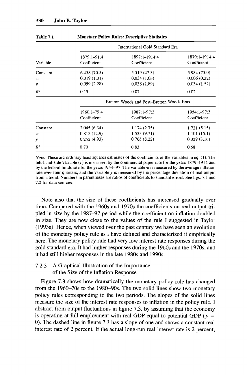
tion about the size of these differences is provided in table 7.
l.
The table shows
least squares estimates of the coefficients on real output (the parameter
g
in
eq.
[
11)
and the inflation rate (the parameter 1
+
h
in eq.
[
11)
for different
time
period^.^
The far right-hand column shows the results for each of the two full periods.
Observe that the estimated values of
g
and 1
+
h
are about
10
times larger in
the Bretton Woods and post-Bretton Woods eras than in the international gold
standard era. It is clear that the gold standard implied much smaller response
coefficients for the interest rate than Federal Reserve policy has implied in
later periods.
8.
Romer
(1986)
demonstrated that biases in the pre-World War
I
data tend
to
overestimate the
volatility in comparison with later periods.
9.
As
explained above this equation is actually a reduced form
of
several structural equations,
especially in
the
gold standard and Bretton Woods periods.
I
have purposely tried to keep the
statistical equations as simple as the theoretical policy rule in
eq.
(1).
No
attempt has been made
to correct the estimates for serial correlation
of
the errors in the equation.
I
want to allow for the
possibility that monetary policy mistakes are serially correlated in ways not necessarily described
by simple time-series models. In fact, this serial correlation is very large, especially in the gold
standard period when
the
equations fit very poorly. Hence, the “t-statistics” in parentheses are not
useful
for hypothesis testing.
See
Christiano, Eichenbaum, and Evans (1997) for a comprehensive
analysis of estimation and identification issues in the case of reaction functions.
330
John
B.
Taylor
Table
7.1
Monetary Policy Rules: Descriptive Statistics
International Gold Standard Era
1879:l-91:4 1897: 1-1914:4 1879: 1-1914:4
Variable Coefficient Coefficient Coefficient
Constant 6.458 (70.5) 5.519 (47.3) 5.984 (75.0)
71
0.019 (1.01) 0.034 (1.03) 0.006 (0.32)
Y
0.059 (2.28) 0.038 (1.89) 0.034
(1.52)
R2
0.15 0.07 0.02
Bretton Woods and Post-Bretton Woods
Eras
1960:l-79:4 1987:l-97:3 1954: 1-97:3
Coefficient Coefficient Coefficient
Constant 2.045 (6.34) 1.174 (2.35) 1.721 (5.15)
7r
0.813 (12.9)
1.533 (9.71) 1.101 (15.1)
V
0.252 (4.93) 0.765 (8.22) 0.329 (3.16)
R2
0.70 0.83 0.58
Note;
These are ordinary least squares estimates of the coefficients of the variables in eq. (I).
The
left-hand-side variable
(r)
is measured by the commercial paper rate for the years 1879-1914 and
by the federal funds rate for the years 1954-97. The variable
T
is measured by the average inflation
rate over four quarters, and the variable
y
is
measured by
the
percentage deviation of real output
from
a
trend. Numbers in parentheses are ratios of coefficients to standard errors. See
figs.
7.1 and
7.2 for data sources.
Note also that the size of these coefficients has increased gradually over
time. Compared with the
1960s
and
1970s
the coefficients on real output tri-
pled in size by the
1987-97
period while the coefficient on inflation doubled
in size. They are now close to the values of the rule
I
suggested in Taylor
(1993a).
Hence, when viewed over the past century we have seen an evolution
of
the monetary policy rule as
I
have defined and characterized it empirically
here. The monetary policy rule had very low interest rate responses during the
gold standard era. It had higher responses during the
1960s
and the
1970s,
and
it had still higher responses in the late
1980s
and
1990s.
7.2.3
A
Graphical Illustration of the Importance
of the Size
of
the Inflation Response
Figure
7.3
shows how dramatically the monetary policy rule has changed
from the
1960-70s
to the
1980-90s.
The two solid lines show two monetary
policy rules corresponding to the two periods. The slopes of the solid lines
measure the size of the interest rate responses to inflation in the policy rule.
I
abstract from output fluctuations in figure
7.3,
by assuming that the economy
is operating at full employment with real
GDP
equal to potential GDP
(y
=
0).
The dashed line in figure
7.3
has a slope of one and shows a constant real
interest rate
of
2
percent.
If
the actual long-run real interest rate is
2
percent,

331
A Historical Analysis
of
Monetary
Policy
Rules
5
Interest Rate
4
3
2
1
0
Monetary Policy
Rule
(1
987-1 997)
\
/
//-
Real rate equals interest
two
percent
Monetary Policy
Rule
(1
960-1
979)
/
I
I
I
1
I
I
1
2
3
4
5
Inflation Rate
Fig.
7.3
Two
estimated monetary policy
rules:
1960-79 versus 1987-97
then the intersection of the dashed line and the policy rule line gives the long-
run average inflation rate.
Observe that the slope of the policy rule has gone from below one to above
one.
A
slope below one would lead to poor economic performance according
to
variety of models. With the slope less than one, an increase in inflation
would bring about a
decrease
in the real interest rate. This would increase de-
mand and add to upward pressures on inflation. This is exactly the wrong pol-
icy response to an increase in inflation because it would lead to ever increasing
inflation. In contrast, if the slope
of
the policy rule were greater than one, an
increase in inflation would bring about an
increase
in the real interest rate,
which would be stabilizing.
These theoretical arguments are illustrated in figure 7.3. For a long-run equi-
librium, we must be at the intersection of the policy rule line and the dashed
line representing the long-run equilibrium real interest rate. If the slope of the
policy rule line is greater than one, higher inflation leads to higher real interest
rates and the inflation rate converges to an equilibrium at the intersection of
the policy rule line and the dashed real interest rate line. For example, if the
equilibrium real interest rate is
2
percent as in figure 7.3, the equilibrium infla-
tion rate is about
1.5
percent for the recent, more steeply sloped, monetary
policy rule in figure 7.3. However, if the slope
of
the policy rule line is less

332
John
B.
Taylor
than one, higher inflation leads to a lower real interest rate, which leads to even
higher inflation; the inflation rate is unstable and would not converge to an
equilibrium. In sum, figure 7.3 shows why the inflation rate would be more
stable
in
the 1987-97 period than in the 1960-79 period.
7.3
Effects
of
the Different Policy Rules
on
Macroeconomic Stability
Can one draw a connection between the different policy rules and the eco-
nomic performance with those policy rules? In particular, within the range
of
policy rules we have seen, is it true that more responsive policy rules lead to
greater economic stability? Making such a connection is complicated by other
factors, such as oil shocks and fiscal shocks, but it is at least instructive to try.
7.3.1
Three Monetary Eras
As
the analysis summarized in table 7.1 indicates, three eras of
U.S.
mone-
tary history can be clearly distinguished by big differences in the degree of
responsiveness of short-term interest rates in the monetary policy rule.
First, during the period from about 1879 to about 1914 short-term interest
rates were very unresponsive to fluctuations in inflation and real output. Sec-
ond, during the period from about 1960 to 1979 short-term interest rates were
more responsive, but still small in the sense that the response of the nominal
interest rate to changes in inflation was less than one. Third, during the period
from about 1986 to 1997 the nominal interest rate was much more responsive
to both inflation and real output fluctuations.
These three eras can also be distinguished in terms of overall economic sta-
bility. Of the three, there is no question that the third had the greatest degree
of economic stability. Figure 7.1 shows that both inflation and real output had
smaller fluctuations during this period. The period contains both the first and
second longest peacetime expansions in
U.S.
history. Moreover, inflation was
low and stable. And, of course, this is the period in which the monetary policy
rule had the largest reaction coefficients, giving support to model-based re-
search that this was a better policy rule than those implied by the two earlier
periods.
The relative ranking of the first and second periods is more ambiguous. Real
output and inflation fluctuations were larger in the earlier period. But while
inflation was more variable, there was much less persistence of inflation during
the gold standard than in the late 1960s and 1970s. However, the different
exchange rate regimes are another monetary factor that must be taken into
account.
It
was the gold standard that kept the long-run inflation rate
so
stable
in the earlier period. Bretton Woods may have provided a similar constraint on
inflation during the early 1960s, but as
U.S.
monetary policy mistakenly be-
came too easy, it was not inflation that collapsed, it was the Bretton Woods
system. And after the end
of
Bretton Woods this external constraint on inflation
was removed. With the double whammy of the loss of an external constraint

333
A
Historical Analysis
of
Monetary Policy Rules
and an inadequately responsive monetary policy rule in place, the inevitable
result was the Great Inflation.
If one properly controls for the beneficial external influences of the gold
standard on long-run inflation during the 1879-1914 period, one obtains an un-
ambiguous correlation between monetary policy rule and macroeconomic sta-
bility. The most economically stable period was the one with the most respon-
sive policy rule. The least economically stable (again adjusting for the gold
standard effects) was the one with the least responsive policy rule. The late
1960s and 1970s
also
rank lower than the most recent period in terms of eco-
nomic stability and had a less responsive monetary policy rule.
7.3.2
In any correlation analysis between economic policy and economic out-
comes there is the possibility of reverse causation. Could the lower respon-
siveness of interest rates in the two earlier periods compared with the later
period have been caused by the greater volatility of inflation and real output?
If one examines the history of changes in the monetary policy rule I think it
becomes clear that the answer is no. The evolution of the monetary policy rule
is best understood as a gradual process
of
the Federal Reserve learning how to
conduct monetary policy. This learning occurred through research by the staff
at the Fed, through the criticism of monetary economists outside the Fed,
through observation of central bank behavior in other countries, and through
direct personal experience of members of the FOMC. And, of course, there
were steps backward as well as fonvard.'O
This learning process occurred as the United States moved further and fur-
ther away from the classical international gold standard. Under the gold stan-
dard, increases and decreases in short-term interest rates were explained by the
interaction of the quantity of money supplied (determined by high-powered
money through the inflow and outflow of gold) and the quantity of money
demanded (which rose and fell as inflation and output rose and fell). A greater
response of the short-term interest rate to rising or falling price levels and to
rising or falling output would probably have reduced the shorter run variability
of inflation and output. For example, lower interest rates during the start of the
deflation period may have prevented the deflation. But because of the fixed
exchange rate feature of the gold standard, the
U.S.
inflation rate was con-
strained to be close to the inflation rates of other gold standard countries; the
degree
of
closeness depended on the size and the duration
of
deviations from
purchasing power parity.
The Federal Reserve started operations at the same time as the classical gold
standard ended: 1914. From the
start
there was therefore uncertainty and dis-
Explaining the Changes in the Policy Rules
10.
If
economists' research on the existence of a long-run trade-off between inflation and unem-
ployment helped lead to the Great Inflation in the 1970s, then this research should be counted as
a step backward.
The
effect of economic research and other factors that may have led to the Great
Inflation
are
discussed in De Long (1997) and in
my
comment on De Long's paper.
334
John
B.
Taylor
agreement about how monetary policy should be conducted without the con-
straints of the gold standard and fixed exchange rates. The Federal Reserve Act
indicated that currency-best interpreted now as the monetary base
or
high-
powered money-was to be elastically provided. But how was the Fed to deter-
mine the degree of this elasticity?
The original idea was that two factors-each pulling in an opposite direc-
tion-were to be balanced out. One was the gold standard itself; with a gold
reserve requirement limiting the amount of Federal Reserve liabilities, the sup-
ply of money was limited. This was a long-run constraint
on
the supply of
money; it worked through gold inflows and gold outflows and the gradual ad-
justment of the
U.S.
price level compared with foreign price levels. The other
factor, which worked more quickly, was “real bills” or “needs of trade” doc-
trine under which the supply of money was to be created in sufficient amounts
to meet the demand for money. Clearly, the needs-of-trade criterion was not
effective on its own because it did not put a limit
on
the amount of money
creation. Therefore, with the suspension of the gold standard and with the real
bills criterion ineffective in determining the supply of money, the Federal Re-
serve began operations with no criteria for determining the appropriate amount
of money to supply. Hence, ever since this uncertain beginning, the Fed has
been searching for such criteria. From the perspective of this paper, we can
think of the Fed as searching for a good monetary policy rule.
This search is evident in many Federal Reserve reports. Early on, the idea
of “leaning against the wind” was discussed as a counterbalance to the needs-
of-trade criterion. For example, the Fed’s annual report for 1923 stated that “it
is the business of the [Federal] Reserve system to work against extremes either
of deflation or inflation and not merely to adapt itself passively to the ups and
downs of business” (quoted in Friedman and Schwartz 1963, 253). But there
was
no
agreement about how much leaning against the wind there should be.
As
discussed above, leaning against the wind would result in a policy rule of
the type in equation
(1),
but the parameters of the policy rule could be far from
optimal. That the Fed was unable throughout the interwar period to find an
effective policy rule for conducting monetary policy is evidenced by the disas-
trous economic performance during the Great Depression when money growth
fell dramatically.
The search for a monetary policy rule was postponed during World War
I1
and in the postwar period by the overriding objective of keeping Treasury
borrowing costs down. (Effectively the Fed set
g
=
0
and
h
=
-1
so
that
r
was a constant stipulated by the
US.
Treasury.) However, after the 1951 Trea-
sury-Federal Reserve Accord, the Fed once again needed a policy rule for
conducting monetary policy. Leaning against the wind-now articulated by
William McChesney Martin-again became a guideline for short-run deci-
sions about changes in the money stock. But the idea was still very vague. As
stated by Friedman and Schwartz (1963) in discussing the mid-1950s when
William McChesney Martin was chairman, “There was essentially no discus-

335
A
Historical Analysis
of
Monetary
Policy
Rules
sion of how to determine which way the relevant wind was blowing.
.
.
.
Nei-
ther was there any discussion of when to start leaning against the wind.
.
. .
There was more comment, but hardly any of it specific about how hard to lean
against the wind”
(63 1-32).
The experience
of
new board member Sherman Maisel indicates that the
search was still going on
10
years later in the
mid-1960s.
According to Maisel
in
his candid memoirs, “After being on the Board for eight months and at-
tending twelve open market meetings,
I
began to realize how far
I
was from
understanding the theory the Fed used to make monetary policy.
.
.
.
Nowhere
did
I
find an account of how monetary policy was made or how it operated”
(1973, 77).
Maisel was particularly concerned about various money market
conditions indexes such as free reserves that came up in Fed deliberations,
because of the difficulty of measuring the impact of these changes on the econ-
omy. He states, “Money market conditions cannot measure the degree to which
markets should be tightened or for how long restraint should be retained”
(82).
And when referring to a decision to raise the short-term interest rate in
1965,
he states, “It became increasingly clear that an inflationary boom was getting
underway and that monetary policy should have been working to curb it”
(81).
However, he argued that the actions taken to raise interest rates were insuffi-
cient to curb the inflation. In retrospect he was correct. Interest rates did not
go
high enough. With no quantitative measure of how high interest rates should
go,
the chance of not raising them high enough was great.
The increased emphasis on money growth in the
1970s
played a very useful
role in clarifying the serious problems
of
interest rate setting without any quan-
titative guidelines. And money growth targets had a very useful role in the
disinflation of the
1979-81
period because it was clear that interest rates would
have to rise by large amounts as the Fed lowered the growth rate of the money
supply. But after the disinflation was over, money growth targets again receded
to being a longer run consideration in Federal Reserve operations as the de-
mand for money appeared to be less stable. Moreover, as noted earlier, ac-
cording to Greenspan’s
(1 997)
analysis, keeping money growth constant does
not give sufficient response of interest rates to inflation or real output when the
aim is to keep inflation low and steady.
The importance
of
having a policy rule to guide policy became even more
important when the Bretton Woods system fell apart in the early
1970s.
Until
then the long-run constraints on monetary policy were similar to those of the
international gold standard.
If
the Fed did not lean hard enough against the
wind, the higher inflation rate would start to put pressure on the exchange rate
and the Fed would have to raise interest rates to defend the dollar. But without
the dollar to defend, this constraint on monetary policy was lost. After Bretton
Woods ended there was an even greater need for the Fed to develop a monetary
policy rule that was sufficient to contain inflation without the external con-
straint. This need was one of the catalysts for the rational expectations econo-
metric policy evaluation research in the
1970s
and
1980s.

336
John
B.
Taylor
This brief review of the evolution of policy indicates that macroeconomic
events, economic research, and policymakers at the Fed have gradually
brought forth changes in the monetary policy rule in the United States.
I
think
this gradual evolution makes it clear that the causation underlying the negative
correlation between the size of the policy response of interest rates to output
or inflation and the volatility of output or inflation goes from policy to out-
come, not the other way around.
If we apply this learning hypothesis to the changes in the estimated policy
rule described above, it suggests that the Federal Reserve learned over time to
have higher response coefficients in a policy rule like equation
(1).
What led
the Fed to change its policy in such a way that the parameter
h
changed from
a negative number to a positive number? Experience with the Great Inflation
of the
1970s
that resulted from a negative value for
h
may be one explanation.
Academic research on the Phillips curve trade-off and the effects of different
policy rules resulting from the rational expectations revolution may be an-
other.
‘‘
7.4
“Policy Mistakes”: Big Deviations
from
Baseline Policy Rules
The historical analysis thus far in this paper has not assumed that any partic-
ular policy rule was better than the others. However, that was the conclusion
of the analysis: a comparison of policy rules and economic outcomes points to
the rule the Fed has been using in recent years as a better way to run monetary
policy than the way it was run in earlier years. That conclusion of the historical
analysis bolsters the very similar conclusion
of
the model-based research sum-
marized in the introduction to this paper.
Once one has focused on a particular policy rule, however, there is another
way to use history to check whether the policy rule would work well. With a
preferred policy rule in hand, one can look at episodes in the past when the
instrument of policy-the federal funds rate in this case-deviated from the
settings given by the preferred policy rule. We can characterize such deviations
as “policy mistakes” and see if the economy was adversely affected as a result
of
these mistakes.I2
Figures
7.4,
7.5,
and
7.6
summarize the results of this historical “policy
mistake” analysis. They show the actual federal funds rate and the value of the
federal funds rate implied by two policy rules. The gap between the actual
11.
Chari, Christiano, and Eichenbaum
(1998)
argue that the Fed was
too
accommodative to
inflation
(h
was too low) in the
1970s
because high expectations of inflation raised the costs
of
disinflation, rather than because the Fed still had something to learn about the Phillips curve trade-
off
or
about the effects of different policy rules.
I
find
the
learning argument more plausible in
part
because it explains the end of the inflation and the change in the policy
rule.
12.
We
are,
of course, looking at these past episodes with the benefit
of
later research and
experience. The term “mistake” does not necessarily mean that policymakers of the past had the
information to do things differently.

337
A
Historical Analysis
of
Monetary Policy
Rules
Percent
l6
1
Fig.
7.4
Federal funds rate: too high in the early
1960s;
too
low
in the late
1960s
Note:
Rules
1
and
2
are given
by
the monetary policy rule in eq.
(1) with
g
=
0.5
and
1.0,
respec-
tively.
Percent
2o
1
..................................................
75 76 77
78
79
80 81
82
83 84 85 86
Fig.
7.5
Federal funds rate: too
low
in the
1970s;
on track in
1979-81;
too high
in
1982-84
Note:
See note to fig.
7.4.
federal funds rate and the policy rules is a measure
of
the policy mistake. One
of
the monetary policy rules
I
use is the one
I
suggested in Taylor (1993a),
which
is
equation
(1)
with the parameters
g
and
h
equal to
0.5.
This is rule
1
in figures
7.4,7.5,
and 7.6.
As
mentioned above, more recent research has sug-
gested that
g
should be closer to
1.0,
giving a more procyclical interest rate.
This variant is rule
2
in the figures.

338 John
B.
Taylor
l2
1
Rule
2
Percent
\
87
88 89
90
91
92
93 94
95
96
97
Fig.
7.6
Federal funds rate: on track in the late
1980s
and
1990s
Nore:
See
note to
fig. 7.4.
The gap between the actual federal funds rate and the policy rule is particu-
larly large in three episodes shown in figures 7.4 and 7.5, especially
in
compar-
ison with the relatively small gap in the late 1980s and 1990s shown in
fig-
ure 7.6.
The first episode occurred in the early 1960s when the mistake was making
monetary policy too tight. Regardless of whether
g
is 0.5 or 1.0 the actual
federal funds rate is well above the policy rule. The gap between the funds rate
and the baseline policy was between
2
and 3 percentage points and this gap
lasted for about three and a half years.I3
It is interesting to note that Friedman and Schwartz (1963, 617) also con-
cluded that monetary policy was overly restrictive during this period. They cite
several reasons why policy may have been too tight. First, the Fed was con-
cerned about the balance
of
payments and an outflow of gold. Second, in look-
ing back at the previous recovery, it appeared to the Fed that policy had eased
too soon after the recession. What was the result of this policy mistake? The
recovery from the 1960-61 recession was weak and the eventual expansion
was slow for several years from about 1962 to 1965.
In
fact, the economy did
not appear to catch up to its potential until 1965. The New Economics intro-
duced by President Kennedy and his economic advisers was addressed at this
prolonged period with real output below potential.
The second episode started in the late 1960s and continued throughout the
1970s-a mistake with
so
much serial correlation it would pass a unit root test!
In this case the monetary policy mistake was being way too easy.
As
shown in
figures 7.4 and
7.5,
the gap between the funds rate and the baseline policy
13.
With its high output response, rule
2
brings the interest rate below zero
for
several quarters,
so
the interest rate is set to
a
small positive number in the chart.

339
A
Historical Analysis
of
Monetary
Policy
Rules
started growing in the late 1960s. It grew as large as 6 percentage points and
persisted in the 4 to 6 percentage point range until the late 1970s when Paul
Volcker took over as Fed chairman. The excessive ease in policy began well
before the oil price shocks of the 1970s, thus raising doubts that these shocks
were the cause of the 1970s Great Inflation.
What caused this monetary policy mistake? Economic research of the
1960s
suggested that there was a long-run trade-off between inflation and unemploy-
ment; this research probably reduced some of the aversion to inflation by the
Federal Reserve. At the least the belief by some in a long-run Phillips curve
made defending low inflation more difficult at the Fed. Note that the mistake
began well before the Friedman-Phelps hypothesis was put forward. Moreover,
as the quotes from Maisel’s memoirs above make clear, the Fed‘s use of money
market conditions caused them to understate the degree of tightness. De
Long
(1997) argues that the overly expansionary policy was due to a great fear of
unemployment carried over from the Great Depression, though he does not
attempt to explain why this mistake occurred when it did. While the causes of
this mistake may be uncertain, there is little doubt that it was responsible for
bringing on the Great Inflation of the 1970s. In my view this mistake is the
second most serious monetary policy mistake in twentieth-century
US.
his-
tory, the most serious being the Great Depression.
If
a policy closer to the
baseline were followed, the rise in inflation may have been avoided.
The third episode occurred after the disinflation of the early 1980s. The in-
crease in interest rates in 1979 and 1980 was about the right magnitude ac-
cording to either of the policy rules. But both rule 1 and rule 2 indicate that
the funds rate should have been lowered more than it was in the 1982-84 pe-
riod. During this period the interest rate was well above the value implied by
the two policy rules. However, it should be emphasized that this period oc-
curred right after the end of the 1970s inflation, and interest rates higher than
recommended by the policy rules may have been necessary to keep expecta-
tions of inflation from rising and to help establish the credibility of the Fed.
In
effect the Fed was in a transition between policy rules. In my view this period
has less claim to being a “policy mistake” than the other two periods.
7.5
Conclusions
The main conclusions of this paper can be summarized as follows. First,
a
monetary policy rule for the interest rate provides a useful framework with
which to examine
U.S.
monetary history.
It
complements the framework pro-
vided by the quantity equation of money so usefully employed by Friedman
and Schwartz (1963). Second, a monetary policy rule in which the interest rate
responds to inflation and real output is an implication
of
many different mone-
tary systems. Third, the monetary policy rule has changed dramatically over
time in the United States, and these changes are associated with equally dra-
340
John
B.
Taylor
matic changes in economic stability. Fourth,
an
examination of the underlying
reasons for the monetary policy changes indicates that they have caused the
changes in economic outcomes, rather than the reverse. Fifth, a monetary pol-
icy rule in which the interest rate responds to inflation and real output more
aggressively than during the 1960s and 1970s
or
than during the international
gold standard-and more like the late 1980s and 1990s-is a good policy rule.
Sixth, if one defines policy mistakes as deviations from such a good policy
rule, then such mistakes have been associated with either high and prolonged
inflation or drawn-out periods
of
low capacity utilization, much as simple mon-
etary theory would predict.
Overall the results of the historical approach in this paper are quite consis-
tent with the results of the model-based approach to monetary policy evalua-
tion. But in an important sense this paper has only touched the surface; many
other issues could be explored with a historical approach. For example, two
difficult problems with monetary policy rules such as equation (1) have been
mentioned by Alan Greenspan (1997): both potential GDP and the real rate
of
interest are uncertain. Uncertainty about the level
of
potential GDP (and the
natural rate of unemployment) is a problem faced by monetary policymakers
today regardless of whether they use a policy rule for guidance. Looking back
at previous episodes and seeing the results of mismeasuring either potential
GDP or the real rate of interest might help reduce the probability
of
making
the next monetary policy mistake.
References
Balke, Nathan
S.,
and Robert J. Gordon. 1986. Appendix B: Historical data.
In
The
American business cycle: Continuity and change,
ed. Robert
J.
Gordon. Chicago:
University of Chicago Press.
Bernanke, Ben, Mark Gertler, and Mark Watson. 1997. Systematic monetary policy and
the effects
of
oil price shocks.
Brookings Papers
on
EconomicActivity,
no.
1:91-157.
Bordo, Michael
D.,
and Anna J. Schwartz. 1999. Monetary policy regimes and eco-
nomic performance: The historical record.
In
Handbook
of
macroeconomics,
ed.
John B. Taylor and Michael Woodford. Amsterdam: North Holland.
Brayton, Flint, Andrew Levin, Ralph Tryon, and John Williams. 1997. The evolution
of
macro models at the Federal Reserve Board.
Curnegie-Rochester Conference Series
on
Public Policy
47:43-81.
Bryant, Ralph, Peter Hooper, and Catherine Mann. 1993.
Evaluating policy regimes:
New
empirical research in empirical macroeconomics.
Washington, D.C.: Brook-
ings Institution.
Cagan, Phillip. 1971. Changes
in
the cyclical behavior of interest rates.
In
Essays on
interest rates,
ed. Jack M. Guttentag. New York: Columbia University Press.
Chari,
V.
V.,
Lawrence Christiano, and Martin Eichenbaum. 1998. Expectation traps
and discretion.
Journal
of
Economic Theory
81
(2): 462-98.
Christiano, Lawrence J., Martin Eichenbaum, and Charles L. Evans. 1997. Monetary
policy shocks: What have we learned and to what end?
In
Handbook
of
macroeco-
nomics,
ed. John B. Taylor and Michael Woodford. Amsterdam: North Holland.

341
A Historical Analysis
of
Monetary Policy Rules
Clarida, Richard, Jordi Gali, and Mark Gertler. 1998. Monetary policy rules in practice:
Some international evidence.
European Economic Review
42: 1033-67.
De Long,
J. Bradford. 1997. America’s peacetime inflation: The 1970s. In
Reducing
injlation: Motivation and strategy,
ed. Christina D. Romer and David
H.
Romer. Chi-
cago: University of Chicago Press.
Friedman, Milton, and Anna Schwartz. 1963.
A monetary history
of
the United States,
1867-1960.
Princeton, N.J.: Princeton University Press.
Greenspan, Alan. 1997. Remarks at the 15th anniversary conference of the Center for
Economic Policy Research. Stanford University,
5
September.
Judd, John F., and Glenn D. Rudebusch. 1998. Taylor’s rule and the Fed: 1970-1997.
Federal Reserve Bank
of
Sun Francisco Economic Review,
no. 3:3-16.
Judd, John F., and Bharat Trehan. 1995. Has the Fed gotten tougher on inflation?
Fed-
eral Reserve Bank
of
San
Francisco Weekly Letter;
no. 95-13.
Maisel, Sherman J. 1973.
Managing the dollar.
New York: Norton.
McCallum, Bennett. 1988. Robustness properties of a rule
for
monetary policy.
Carne-
gie-Rochester Conference Series
on
Public Policy
29:
173-203.
McKinnon, Ronald I., and Kenichi Ohno. 1997.
Dollar and yen.
Cambridge, Mass.:
MIT Press.
Romer, Christina D. 1986. Is the stabilization of the postwar economy a figment
of
the
data?
American Economic Review
76:3 14-34.
Romer, Christina D., and David Romer. 1989. Does monetary policy matter? A new
test in the spirit of Friedman and Schwartz. In
NBER macroeconomics annual
1989,
ed.
0.
J. Blanchard and
S.
Fischer. Cambridge, Mass.: MIT Press.
Sargent, Thomas. 1986. The end
of
four big inflations. In
Rational expectations and
inflation,
ed. Thomas Sargent, 40-109. New York: Harper and Row.
Sims, Christopher, and Tao Zha. 1995. Does monetary policy generate recessions? At-
lanta: Federal Reserve Bank of Atlanta. Working paper.
Taylor, John B. 1979. Estimation and control of a macroeconomic model with rational
expectations.
Econometrica
47
(5):
1267-86.
.
1993a. Discretion versus policy rules in practice.
Carnegie-Rochester Confer-
ence Series
on
Public Policy
39:195-214.
.
1993b.
Macroeconomic policy in a world economy: From econometric design
to practical application.
New York: Norton.
Comment
Richard H. Clarida
It is a pleasure to discuss this paper by John Taylor. In it, he proposes to use
the Taylor rule as an analytical framework for the interpretation
of
monetary
history, much as Friedman and Schwartz employed the quantity equation.
I
agree with the approach that he is trying to promote,
I
concur in general with
the inferences he draws from it, and
I
believe that this way of interpreting
monetary history can be, and in my work with Jordi Gali and Mark Gertler
(1998a, 1998b) has already been, applied in fruitful ways that complement the
application emphasized in this paper.
Richard
H.
Clarida is professor
of
economics and international affairs and chairman
of
the
Department of Economics, Columbia University.

342
John
B.
Taylor
The basic idea is straightforward, and much of the paper is devoted to justi-
fying its application. A baseline, or reference, time path of the short-term (fed-
eral funds) interest rate is constructed using a Taylor (1993) rule of the form
r,
=
rf
+
rr*
+
h(q
-
TT*)
+
gy,,
where
ri
is the long-run equilibrium real interest rate,
TT*
is the long-run equi-
librium rate of inflation, and
y,
is the output gap. After the baseline is con-
structed, the actual time path of the short-term interest rate is compared to the
baseline path. Episodes (i.e., sequences of observations) in which the funds
rate is persistently higher than the baseline path are interpreted as episodes of
excessively “tight” monetary policy, while episodes in which the funds rate is
consistently below the baseline are interpreted as episodes in which monetary
policy is too “easy.” Although Taylor provides some qualification in footnote
12,
he is explicit in his interpretation of these episodes of “easy” and “tight”
policy as representing policy mistakes.
Now if, as we have learned from the central bankers present at this confer-
ence, the Taylor rule can be and is used as a benchmark for assessing the cur-
rent stance of actual monetary policies, then certainly it can also be used as
part of a framework to interpret monetary history. But certainly the caveats that
apply to its use as a benchmark for current policy also apply, and perhaps with
even greater force, to its use as a framework for interpreting monetary history.
Unobservable but essential inputs to the Taylor rule such as the equilibrium
real interest rate and the NAIRU fluctuate over time. Data get revised, and with
these revisions the amplitudes-and sometimes the signs-of business cycle
indicators appear much different with hindsight than they did to contemporar-
ies. Taylor’s paper exhibits the appreciation and awareness of these issues that
I
would expect of him, and subsequent authors that pursue this approach would
do well
to
emulate him.
As applied to U.S. monetary policy since 1960,
I
believe Taylor’s interpreta-
tions are largely correct. In fact, my paper with Jordi Gali and Mark Gertler
(1998a) makes very similar points using
an
estimated version of what we call
a “forward-looking’’ Taylor rule. A forward-looking Taylor rule estimated over
the post-1979 period-with
h
=
1.96 and
g
=
0.07-captures all the major
swings in the funds rate. When we backcast the post-1979 rule on the pre-1979
data, we also infer-as does Taylor-that policy was “too easy” between 1965
and 1979. Indeed, our parameter estimates for the 1960-79 period
(h
=
0.80
and
g
=
0.52)
confirm Taylor’s interpretation that the source of the 1965-79
policy mistake was that the Fed, when faced with
an
increase in inflation,
raised the funds rate,
but by less than the rise in injation
so
that a rise in
inflation was countered by a fall in the real interest rate.
This finding is per-
fectly consistent with, indeed it can be viewed as the explanation for, Mishkin’s
(1981) famous empirical result that during the 1970s the ex ante real interest
rate varied inversely with inflation.

343
A
Historical
Analysis
of
Monetary Policy Rules
Why is it that before 1979, the Fed appears to have followed a policy that,
with hindsight, was clearly inferior to the policy it has followed since? Ac-
cording to Clarida
et
al.:
Another way to look at the issue is to ask why it is that the Fed maintained
persistently low short term real rates in the face of high or rising inflation.
One possibility, emphasized by DeLong (1997), is that the Fed thought the
natural rate of unemployment at this time was much lower [and potential
output higher] than it really was.
. .
.
Another
.
. .
possibility is that, at the
time, neither the Fed nor the economics profession understood the dynamics
of inflation very well. Indeed, it was not until the mid-to-late 1970s that.
.
.
textbooks began emphasizing the absence of a long run trade-off between
inflation and output. The idea that expectations may matter in generating
inflation and that credibility is important in policy-making were simply not
well established during that era. What all this suggests
is
that in understand-
ing historical economic behavior, it is important to take into account the
state of policy-maker’s knowledge of the economy and how it may have
evolved over time. Analyzing policy-making from this perspective, we
think, would be a highly useful undertaking. (1998a,
24)
To this, I might add that I believe policymakers and the profession only began,
in the late 196Os, to appreciate the distinction between movements in nominal
and real interest rates.
As Taylor suggests in his paper, a systematic policy of raising the funds rate
by less than inflation “would ultimately imply an unstable inflation rate.” In
Clarida et al. (1998a), we embed a forward-looking Taylor rule with
h
<
1 in
a version of the sticky price models found in King and Wolman (1996), Wood-
ford (1996), and McCallum and Nelson (chap. 1 of this volume). We find that
for
h
<
1, there can be bursts of inflation and output fluctuations that result
from self-fulfilling changes in expectations. These sunspot fluctuations may
arise because under this rule individuals correctly anticipate that the Fed will
accommodate a rise in expected inflation by letting real interest rates decline.
These sunspot fluctuations do not arise when
h
>
1.
As Taylor mentions in his paper, in Clarida et al. (1998b), we introduce
another way to use the Taylor rule baseline to interpret recent monetary history.
Specifically, we interpret the collapse in September 1992
of
the European
Monetary System
(EMS)
by calculating for France, Italy, and Britain during
the several years leading up to and several years following the collapse a stress
indicator defined as
fltr
stress,,,
=
r,.,
-
J.l
’
When
stressj,t
is
positive, short-term interest rates in country
j
are higher than
they would be if they were set according to a Taylor rule based on inflation and
output in country
j.
Does this mean that monetary policy in country
j
is “too
tight”? In this instance no, because with the dismantling of capital controls in
the
1990s,
these countries’ decisions to fix their exchange rates meant they

344
John
B.
Taylor
gave up autonomy over their national monetary policies. The
EMS
evolved
into a system in which Germany set the level of interest rates for all member
countries; any remaining fluctuations in country-specific interest differentials
with Germany reflected the changing sentiments of speculators regarding the
commitment of that country to the fixed exchange rate. How then do we inter-
pret a positive reading
of
stress? It is a measure, in basis points, of the cost to
country
j
of belonging to a fixed exchange rate system when monetary policy
is not being set based on the macroeconomic conditions in country
j.
References
Clarida, R.,
J.
Gali, and
M.
Gertler. 1998a. Monetary policy rules and macroeconomic
stability: Evidence and some theory. NBER Working Paper no. 6442. Cambridge,
Mass.: National Bureau of Economic Research.
. 1998b. Monetary policy rules in practice: Some international evidence.
Euro-
pean Economic Review
42: 1033-67.
King, R., and A. Wolman. 1996. Inflation targeting in
a
St. Louis model
of
the 21st
century. NBER Working Paper no. 5507. Cambridge, Mass.: National Bureau of Eco-
nomic Research.
Mishkin,
F.
1981. The real interest rate: An empirical investigation.
Carnegie-Rochester
Conference Series
on
Public Policy
15:
151-200.
Taylor,
J.
1993. Discretion versus policy rules in practice.
Cumegie-Rochester Confer-
ence Series
on
Public Policy
39:195-214.
Woodford, M. 1996. Control of the public debt: A requirement for price stability'?
NBER Working Paper
no.
5684. Cambridge, Mass.: National Bureau
of
Economic
Research.
Discussion
Summary
Laurence Bull
asked Taylor for his conjecture on how much of the economy's
better performance under Alan Greenspan than under Arthur Bums was attrib-
utable to optimal policy and how much to better luck in the sense of not experi-
encing the Vietnam War and two oil shocks. This could be addressed formally
by decomposing output variance into the variance of shocks and variance
caused by deviations from the optimal rule.
Taylor
replied that his view on this
issue was influenced by De Long
(1997),
who indicates that the policy mistake,
under this definition, began well before the oil shocks.
A
more responsive pol-
icy rule could have led to a bigger decline in output during the first oil shock,
but it is quite likely that inflation would not have risen
so
much. Thus the econ-
omy would have gotten away with a much smaller disinflation in the early
1980s.
Bull
then questioned the result that policy was too tight in
1983,
whereas
there was a rapid recovery going on during that time.
Taylor
responded that the
policy mistake had already occurred at the beginning of
1982.
While the gen-

345
A
Historical Analysis
of
Monetary Policy
Rules
era1 raising
of
interest rates by Volcker during
1979-81
was about right, the
funds rate should have been lowered by a greater amount when the economy
really sank.
Glenn Rudebusch
expressed doubts as to whether another measure
of output gap rather than the one used in the paper would have shown such a
deep recession for
1982.
Taylor
replied that the gap obtained with the Hodrick-
Prescott filter looked similar to the one in Judd and Trehan
(1995).
Martin
Feldstein
mentioned that part
of
the reason for overtight interest rates at that
point was that Volcker felt keeping up with the disinflation for much longer
was politically unsustainable; hence,
the
disinflation had to occur in
a
shorter
than optimal length of time.
Edward Gramlich
mentioned that Volcker shifted
from the money to the funds standard during that period. This happened at
least in part because there was a shift in money demand due to, for example,
interest payments on demand deposits.
Donald Kohn
added that money growth
was accelerating toward the end of
1982
and inflation expectations were persis-
tently high, much higher than ex post realized inflation.
Frederic Mishkin
added that after
a
history of bad policy, Volcker wanted to be tough in order to
gain credibility.
Ben McCallum
mentioned that the Federal Reserve was below
its
M1
target in
1981.
William
Poole
stressed that the economy sank much
more quickly than anybody anticipated in
1982.
There was an enormous inven-
tory runoff, and the unemployment rate shot up in literally two months.
Bob
Hall
noted that during the national bank era, prior to the creation of the
Federal Reserve, the control of the price level was through the commodity
definition of the dollar. Federal involvement in the portfolio sense of control-
ling the quantity
of
money was only indirect, through the national bank notes.
Hall expressed concern about the fact that the paper repeats what he sees as
the mistake of Friedman and Schwartz in trying to understand the commodity
standard as if it were a portfolio-based monetary standard.
Tuylor
replied that
the gold standard kept the price level stable during that period through the
pressure of purchasing power parity, similar to the early time in Bretton Woods.
Michael Woodford
remarked that the coefficient on inflation for the nine-
teenth-century period was even lower than in the
1970s.
The Gibson paradox
suggests that under the gold standard, interest rates seem to be related to the
price level rather than the inflation rate. Even if interest rates rise with the price
level but are not associated with the inflation rate, the real rate does not need
to fall since the inflation rate and even the price level were mean reverting
during that period.
Robert King
wondered about the determination
of
the trend in inflation with
an interest rate rule. Under the monetarist, Friedman and Schwartz interpreta-
tion the trend in money growth determines the trend in inflation.
Taylor
sug-
gested thinking about the policy rule as an inverted money demand equation.
An
inflation coefficient greater than one will generate a stable inflation rate. If
inflation rises, real interest rates rise in the same way as with a money-based
rule. Therefore, this is not inconsistent with the money-based view on the de-
termination of the inflation rate.

346
John
B.
Taylor
King
then noted that an output gap measured by the Hodrick-Prescott filter
implied that the Federal Reserve had to react to output in the future.
Taylor
agreed but reminded him that already with revised data, as mentioned by Don-
ald Kohn before, policy rules look very different than with actual data.
Martin Feldstein
remarked that Taylor rightly stresses, and the diagrams in
the paper nicely show, that the response coefficient on inflation has to be
greater than one,
so
that when inflation increases, real rates rise. In the 1960s
and 1970s, for the reasons given by De Long (1997), the focus was too much
on nominal rates. Even though nominal rates were tightened, real rates were
going down. However, what really matters are the real net rates as shown in
the following equation:
R,
=
(1
-
0)’
1
-
IT.
If
the nominal rate,
i,
is raised one to one with inflation,
IT,
the real net rate,
R,,
falls by the marginal tax rate coefficient
8.
If the real net rate should rise
when inflation goes up, the derivative of
i
with respect
to
T
has to be at least
equal to 1/(1
-
0).
The coefficient
0
is equal to
1/3,
which means that in the
policy rule, the coefficient on inflation should be greater than one. Of course,
there are a lot of markets in which taxes do not matter or for some players the
marginal tax rate is higher than that,
so
this makes not too much of a point
about a value of exactly
1/3
for
8,
but it makes a point that the coefficient
on
inflation should be greater than one and that
1.5
might not be a bad number
at all.
Poole
recalled that in the early 1970s, Friedman’s natural rate hypothesis did
not sweep the profession instantaneously. Year after year, prominent members
of the profession came to the academic consultants’ meetings reporting that
this was a nice theoretical idea, but that in practice there was a long-mn trade-
off between unemployment and inflation. The real rate of interest was not yet
a variable in the Federal Reserve’s macromodel, built in the mid-l960s, until
its revision in 1968. The influence of fiscal policy on aggregate demand was
vastly overestimated. The potential impact of tight money on housing and
fis-
cal policy-all sorts of excuses were made to delay actions. It was not until
1975,
the end
of
the Bums era, that the Federal Reserve finally decided that
the long-run Phillips curve was indeed vertical.
Ben
McCallum
noted that Tay-
lor (1996) supports the point just made.
A
small piece of documentation is a
long speech about inflation written by Arthur Bums and published by the Fed-
eral Reserve Bank of Richmond during the late 1970s. In that 20-page docu-
ment, monetary policy is not mentioned in any shape or form.
McCallum liked Taylor’s approach of running a policy rule through history
and encouraged further research in this direction.
John
Lipsky
pointed out that market participants have paid increasing atten-
tion to the Taylor rule formulation as an indicator of the appropriateness of Fed
policy. Its predictive power has been extremely impressive over the past few

347
A Historical Analysis
of
Monetary Policy Rules
years. Lipsky conjectured that the deregulation
of
financial markets and perva-
sive securitization is enhancing the linkage between the real economy, policy,
and financial markets. Thus the impact
of
monetary policy has been boosted,
underscoring the importance
of
research on potential policy rules like the Tay-
lor
rule.
References
De Long, J. Bradford. 1997. America’s peacetime inflation: The 1970s. In
Reducing
injation: Motivation and strategy,
ed. Christina Romer and David Romer. Chicago:
University
of
Chicago Press.
Judd, John F., and Bharat Trehan. 1995. Has the Fed gotten tougher on inflation?
Fed-
eral Reserve
Bank
of
San Francisco Weekly LRtter;
no. 95-13.
Taylor, John. 1996. How should monetary policy respond
to
shocks while maintaining
long-run price stability?-Conceptual issues. In
Achieving price stabizity.
Kansas
City: Federal Reserve Bank
of
Kansas City.

This Page Intentionally Left Blank
