
Measuring the Macroeconomic Impact of
Monetary Policy at the Zero Lower Bound
Jing Cynthia Wu
Chicago Booth and NBER
Fan Dora Xia
Merrill Lynch
Paper presented at the 16th Jacques Polak Annual Research Conference
Hosted by the International Monetary Fund
Washington, DC─November 5–6, 2015
The views expressed in this paper are those of the author(s) only, and the presence
of the
m, or of links to them, on the IMF website does not imply that the IMF, its
Executive Board, or its management endorses or shares the views expressed in the
paper.
1
1
6
6
T
T
H
H
J
J
A
A
C
C
Q
Q
U
U
E
E
S
S
P
P
O
O
L
L
A
A
K
K
A
A
N
N
N
N
U
U
A
A
L
L
R
R
E
E
S
S
E
E
A
A
R
R
C
C
H
H
C
C
O
O
N
N
F
F
E
E
R
R
E
E
N
N
C
C
E
E
N
N
O
O
V
V
E
E
M
M
B
B
E
E
R
R
5
5
–
–
6
6
,
,
2
2
0
0
1
1
5
5

Working Paper No. 13-77
Measuring the Macroeconomic Impact of Monetary
Policy at the Zero Lower Bound
Jing Cynthia Wu
University of Chicago Booth School of Business
Fan Dora Xia
University of California, San Diego
All rights reserved. Short sections of text, not to exceed two paragraphs. May be quoted without
Explicit permission, provided that full credit including notice is given to the source.
This paper also can be downloaded without charge from the
Social Science Research Network Electronic Paper Collection:
http://ssrn.com/abstract=2321323

Measuring the Macroeconomic Impact of Monetary
Policy at the Zero Lower Bound
∗
Jing Cynthia Wu
Chicago Booth and NBER
Fan Dora Xia
Merrill Lynch
First draft: August 19, 2013
This draft: May 18, 2015
Abstract
This paper employs an approximation that makes a nonlinear term structure model
extremely tractable for analysis of an economy operating near the zero lower bound for
interest rates. We show that such a model offers an excellent description of the data
compared to the benchmark model and can be used to summarize the macroeconomic
effects of unconventional monetary policy. Our estimates imply that the efforts by the
Federal Reserve to stimulate the economy since July 2009 succeeded in making the
unemployment rate in December 2013 1% lower, which is 0.13% more compared to the
historical behavior of the Fed.
Keywords: monetary policy, zero lower bound, unemployment, shadow rate, dynamic
term structure model
JEL classification codes: E43, E44, E52, E58
∗
We have benefited from extensive discussions with Jim Hamilton and Drew Creal. We also thank
Jim Bullard, John Cochrane, Greg Duffee, Benjamin Friedman, Refet Gurkaynak, Kinda Hachem, Anil
Kashyap, Leo Krippner, Randy Kroszner, Jun Ma, David Romer, Glenn Rudebusch, Jeff Russell, Frank
Schorfheide, Matthew Shapiro, Eric Swanson, Ruey Tsay, Ken West, Johannes Wieland, John Williams,
three anonymous referees, and seminar and conference participants at Chicago Booth, UCSD, NBER Summer
Institute Monetary Economics Workshop, St. Louis Fed Applied Time Series Econometrics Workshop,
FRBSF ZLB workshop, Second BIS Research Network meeting, Atlanta Fed, Boston Fed, Chicago Fed,
Dallas Fed, and Kansas City Fed for helpful suggestions. Cynthia Wu gratefully acknowledges financial
support from the IBM Faculty Research Fund at the University of Chicago Booth School of Business.
1
1 Introduction
Historically the Federal Reserve has used the federal funds rate as the primary instrument of
monetary policy, lowering the rate to provide more stimulus and raising it to slow economic
activity and control inflation. But since December 2008, the federal funds rate has been near
zero, so that lowering it further to produce more stimulus has not been an option. Conse-
quently, the Fed has relied on unconventional policy tools such as large-scale asset purchases
(commonly known as quantitative easing) and forward guidance to try to affect long-term
interest rates and influence the economy. Assessing the impact of these measures or sum-
marizing the overall stance of monetary policy in the new environment has proven to be a
big challenge. Previous efforts include Gagnon, Raskin, Remache, and Sack(2011), Hamil-
ton and Wu(2012), Krishnamurthy and Vissing-Jorgensen(2011), D’Amico and King(2013),
Wright(2012), Bauer and Rudebusch(forthcoming), and Swanson and Williams(forthcoming).
However, these papers only focused on measuring the effects on the yield curve. In contrast,
the goal of this paper is to assess the overall effects on the economy.
A related challenge has been to describe the relations between the yields on assets of
different maturities in the new environment. The workhorse model in the term structure
literature has been the Gaussian affine term structure model (GATSM); for surveys, see
Piazzesi(2010), Duffee(forthcoming), G¨urkaynak and Wright(2012), and Diebold and Rude-
busch(2013). However, because this model is linear in Gaussian factors, it potentially allows
nominal interest rates to go negative and faces real difficulties in the zero lower bound (ZLB)
environment. One approach that could potentially prove helpful for both measuring the ef-
fects of policy and describing the relations between different yields is the shadow rate term
structure model (SRTSM) first proposed by Black(1995). This model posits the existence
of a shadow interest rate that is linear in Gaussian factors, with the actual short-term in-
terest rate the maximum of the shadow rate and zero. However, the fact that an analytical
solution to this model is known only in the case of a one-factor model makes using it more
challenging.
2

In this paper we propose a simple analytical representation for bond prices in the multi-
factor SRTSM that provides an excellent approximation and is extremely tractable for anal-
ysis and empirical implementation. It can be applied directly to discrete-time data to gain
immediate insights into the nature of the SRTSM’s predictions. We demonstrate that this
model offers an excellent empirical description of the recent behavior of interest rates, as
compared to the benchmark GATSM.
More importantly, we show using a simple factor-augmented vector autoregression (FAVAR)
that the shadow rate calculated by our model exhibits similar dynamic correlations with
macro variables of interest in the period since July 2009 as the fed funds rate did in data
prior to the Great Recession. This result gives us a tool for measuring the effects of mon-
etary policy at the ZLB, and offers an important insight to the empirical macro literature
where people use the effective federal funds rate in vector autoregressive (VAR) models to
study the relationship between monetary policy and the macroeconomy. Examples of this
literature include Christiano, Eichenbaum, and Evans(1999), Stock and Watson(2001), and
Bernanke, Boivin, and Eliasz(2005). The evident structural break in the effective fed funds
rate prevents researchers from extracting meaningful information out of a VAR once the data
covers the ZLB period. In contrast, the continuity of our shadow rate allows researchers to
update their favorite VAR during and post the ZLB period.
1
We show that the Fed has used unconventional policy measures to successfully lower the
shadow rate, and these measures have been more stimulative than a historical version of the
Taylor rule. Our estimates imply that the Fed’s efforts to stimulate the economy since July
2009 have succeeded in lowering the unemployment rate by 1% in December 2013, which is
0.13% more compared to the historical behavior of the Fed.
The SRTSM has been used to describe the recent behavior of interest rates and mone-
tary policy by Kim and Singleton(2012) and Bauer and Rudebusch(2013), but these authors
1
Our shadow rate data with monthly update is available at the Atlanta Fed (https://www.frbatlanta.
org/cqer/researchcq/shadow_rate.cfm) or our webpage (http://faculty.chicagobooth.edu/jing.
wu/research/data/WX.html).
3
relied on simulation methods to estimate and study the model. Krippner(2013) proposed a
continuous-time analog to our solution, where he added a call option feature to derive the so-
lution. Ichiue and Ueno(2013) derived similar approximate bond prices by ignoring Jensen’s
inequality. Both derivations are in continuous time, which requires numerical integration
when applied to discrete-time data.
Our paper also contributes to the recent discussion on the usefulness of the shadow rate as
a measure for the stance of monetary policy. Christensen and Rudebusch(2014) and Bauer
and Rudebusch(2013) pointed out that the estimated shadow rate varied across different
models. We confirm that different model choices do influence the level of the shadow rate.
However, the common dynamics among different shadow rates point to the same economic
conclusion. We also demonstrate that the shadow rate is a powerful tool to summarize
useful information at the ZLB. Therefore, our evidence further supports the view expressed
by Bullard(2012) and Krippner(2012), who advocated the potential of the shadow rate to
describe the monetary policy stance. Recent work by Lombardi and Zhu(2014) shares the
same view with a shadow rate constructed from a factor model with a large information set.
The rest of the paper proceeds as follows. Section 2 describes the SRTSM. Section 3
proposes to use the shadow rate to measure the monetary policy at the ZLB. Section 4
summarizes the implication of unconventional monetary policy on the macroeconomy using
historical data from 1960 to 2013, and Section 5 zooms in on the ZLB period, and analyses
forward guidance and quantitative easing. Section 6 extends the robustness of our results to
different model specifications, and Section 7 concludes.
4

2 Shadow rate term structure model
2.1 Shadow rate
Similar to Black(1995), we assume that the short term interest rate is the maximum of the
shadow rate s
t
and a lower bound r:
r
t
= max(r, s
t
). (1)
If the shadow rate s
t
is greater than the lower bound, then s
t
is the short rate. Note that
when the lower bound is binding, the shadow rate contains more information about the
current state of the economy than does the short rate itself. Since the end of 2008, the
Federal Reserve has paid interest on reserves at an annual interest rate of 0.25%, proposing
the choice of r = 0.25%.
2
2.2 Factor dynamics and stochastic discount factor
We assume that the shadow rate s
t
is an affine function of some state variables X
t
,
s
t
= δ
0
+ δ
0
1
X
t
. (2)
The state variables follow a first order vector autoregressive process (VAR(1)) under the
physical measure (P):
X
t+1
= µ + ρX
t
+ Σε
t+1
, ε
t+1
∼ N(0, I). (3)
The log stochastic discount factor is essentially affine as in Duffee(2002)
M
t+1
= exp
−r
t
−
1
2
λ
0
t
λ
t
− λ
0
t
ε
t+1
, (4)
2
Our main results are robust if we estimate r as a free parameter, see Section 6 for detailed discussion.
5
where the price of risk λ
t
is linear in the factors
λ
t
= λ
0
+ λ
1
X
t
.
This implies that the risk neutral measure (Q) dynamics for the factors are also a VAR(1):
X
t+1
= µ
Q
+ ρ
Q
X
t
+ Σε
Q
t+1
, ε
Q
t+1
Q
∼ N(0, I). (5)
The parameters under the P and Q measures are related as follows:
µ −µ
Q
= Σλ
0
,
ρ −ρ
Q
= Σλ
1
.
2.3 Forward rates
Equation (1) introduces non-linearity into an otherwise linear system. A closed-form pricing
formula for the SRTSM described in Sections 2.1 - 2.2 is not available beyond one factor.
In this section, we propose an analytical approximation for the forward rate in the SRTSM,
making the otherwise complicated model extremely tractable. Our formula is simple and
intuitive, and we will compare it to the solution from a Gaussian model in Section 2.4. A sim-
ulation study in Section 2.6 demonstrates that the error associated with our approximation
is only a few basis points.
Define f
n,n+1,t
as the forward rate at time t for a loan starting at t + n and maturing at
t + n + 1,
f
n,n+1,t
= (n + 1)y
n+1,t
− ny
nt
, (6)
which is a linear function of yields on risk-free n and n + 1 period pure discount bonds. The
6

forward rate in the SRTSM described in equations (1) to (5) can be approximated by
f
SRT SM
n,n+1,t
= r + σ
Q
n
g
a
n
+ b
0
n
X
t
− r
σ
Q
n
, (7)
where (σ
Q
n
)
2
≡ Var
Q
t
(s
t+n
). The function g(z) ≡ zΦ(z)+φ(z) consists of a normal cumulative
distribution function Φ(.) and a normal probability density function φ(.). Its non-linearity
comes from moments of the truncated normal distribution. The expressions for a
n
, b
n
and
σ
Q
n
as well as the derivation are in Appendix A.
To our knowledge, we are the first in the literature to propose an analytical approxima-
tion for the forward rate in the SRTSM that can be applied to discrete-time data directly.
For example, Bauer and Rudebusch(2013) used a simulation-based method. Krippner(2013)
proposed an approximation for the instantaneous forward rate in continuous-time. To ap-
ply his formula to the one-month ahead forward rate in the data, a researcher needs to
numerically integrate the instantaneous forward rate over that month, see Christensen and
Rudebusch(2014) for example. Conversely, our discrete-time formula can be applied directly
to the data. In summary, our analytical approximation is free of any numerical error asso-
ciated with simulation methods and numerical integration.
2.4 Relation to Gaussian Affine Term Structure Models
If we replace equation (1) with
r
t
= s
t
,
the SRTSM becomes a GATSM, the benchmark model in the term structure literature. The
forward rate in the GATSM is an affine function of the factors:
f
GAT SM
n,n+1,t
= a
n
+ b
0
n
X
t
, (8)
7

where a
n
and b
n
are the same as in equation (7), and the detailed expressions are in Appendix
A.
The difference between (7) and (8) is the function g(.). We plot it in Figure 1 together
with the 45 degree line. It is a non-linear and increasing function. The function value is
indistinguishable from the 45 degree line for inputs greater than 2, and is practically zero
for z less than −2. The limiting behavior demonstrates that the GATSM is a simple and
close approximation for the SRTSM, when the economy is away from the ZLB.
2.5 Estimation
State space representation for the SRTSM We write the SRTSM as a nonlinear state
space model. The transition equation for the state variables is equation (3). From equation
(7), the measurement equation relates the observed forward rate f
o
n,n+1,t
to the factors as
follows:
f
o
n,n+1,t
= r + σ
Q
n
g
a
n
+ b
0
n
X
t
− r
σ
Q
n
+ η
nt
, (9)
where the measurement error η
nt
is i.i.d. normal, η
nt
∼ N (0, ω). The observation equation
is not linear in the factors. We use the extended Kalman filter for estimation, which applies
the Kalman filter by linearizing the nonlinear function g(.) around the current estimates.
See Appendix B for details.
The extended Kalman filter is extremely easy to apply due to the closed-form formula
in equation (7). We take the observation equation (9) directly to the data without any fur-
ther numerical approximation, which is necessary for pricing formulas derived in continuous
time. The likelihood surface behaves similarly to a GATSM, because the function g(.) is
monotonically increasing. These features together make our formula appealing.
8

State space representation for the GATSM For the GATSM described in Section 2.4,
equation (3) is still the transition equation. Equation (8) implies the measurement equation:
f
o
n,n+1,t
= a
n
+ b
0
n
X
t
+ η
nt
, (10)
with η
nt
∼ N (0, ω). We apply the Kalman filter for the GATSM, because it is a linear
Gaussian state space model. See Appendix B for details.
Data We construct one-month forward rates for maturities of 3 and 6 months, 1, 2, 5, 7
and 10 years from the G¨urkaynak, Sack, and Wright(2007) dataset, using observations at
the end of the month.
3
Our sample spans from January 1990 to December 2013.
4
We plot
the time series of these forward rates in Figure 2. In December 2008, the Federal Open
Market Committee (FOMC) lowered the target range for the federal funds rate to 0 to 25
basis points. We refer to the period from January 2009 to the end of the sample as the ZLB
period, and highlight with shaded area. For this period, forward rates of shorter maturities
are essentially stuck at zero, and do not display meaningful variation. Those with longer
maturities are still far away from the lower bound, and display significant variation.
Normalization The consensus in the term structure literature is that three factors are
sufficient to account for almost all of the cross-sectional variation in yields. Therefore, we
focus our discussion on three factor models.
5
The collection of parameters we estimate
include (µ, µ
Q
, ρ, ρ
Q
, Σ, δ
0
, δ
1
). For identification, we impose normalizing restrictions on the
Q parameters similar to Joslin, Singleton, and Zhu(2011) and Hamilton and Wu(2014): (i)
δ
1
= [1, 1, 0]
0
; (ii) µ
Q
= 0; (iii) ρ
Q
is in real Jordan form with eigenvalues in descending order;
3
As a robustness check, we also estimate the SRTSM and extract the shadow rate with Fama and
Bliss(1987) zero coupon bond data from CRSP, and we get similar results. See Section 6 for detailed
discussion.
4
Starting the sample from 1990 is standard in the GATSM literature, see Wright(2011) and Bauer,
Rudebusch, and Wu(2012) for examples.
5
All of our main results relating to the macroeconomy, from Section 3 onward, are robust to two-factor
models, see Section 6 for further discussion. But for the term structure models themselves, two-factor models
perform worse than three-factor models in terms of fitting the data.
9
and (iv) Σ is lower triangular. Note that these restrictions are for statistical identification
only, i.e. they prevent the latent factors from shifting, rotating and scaling. Imposing this
or other sets of restrictions does not change economic implications of the model.
Repeated eigenvalues Estimation assuming that ρ
Q
has three distinct eigenvalues pro-
duces two smaller eigenvalues almost identical to each other, with the difference in the order
of 10
−3
. This evidence points to repeated eigenvalues. Creal and Wu(2015) have docu-
mented a similar observation using a different dataset and a different model. With repeated
eigenvalues, the real Jordan form becomes
ρ
Q
=
ρ
Q
1
0 0
0 ρ
Q
2
1
0 0 ρ
Q
2
.
Model comparison Maximum likelihood estimates, and robust standard errors (See Hamil-
ton(1994) p. 145) are reported in Table 1. The log likelihood value is 755.46 for the GATSM,
and 855.57 for the SRTSM. The superior performance of the SRTSM comes from its ability
to fit the short end of the forward curve when the lower bound binds. In Figure 3, we plot
average observed (red dots) and fitted (blue curves) forward curves in 2012. The left panel
illustrates that the SRTSM fitted forward curve flattens at the short end, because the g(.)
function is very close to zero when the input is sufficiently negative. This is consistent with
the feature of the data. In contrast, the GATSM in the right panel has trouble fitting the
short end. Instead of having a flat short end as the data suggest, the GATSM generates too
much curvature. That is the only way it can approximate the yield curve at the ZLB.
As demonstrated in Section 2.4, the GATSM is a good approximation for the SRTSM
when forward rates are sufficiently higher than the lower bound. We illustrate this property
using the following numerical example. When both models are estimated over the period
of January 1990 to December 1999, the maximum log likelihood is 475.71 for the SRTSM,
10

and 476.69 for the GATSM. The slight difference in the likelihood comes from the linear
approximation of the extended Kalman filter.
2.6 Approximation error
An alternative to equation (7) to compute forward rates or yields is simulation. We compare
forward rates and yields implied by equation (7) and by an average of 10 million simulated
paths to measure the size of the approximation error.
6
The approximation errors grow
with the time to maturity for both forward rates and yields. We focus on the longest end to
report the worst case scenario. The average absolute approximation error of the 24 Januaries
between 1990 and 2013 for the 10-year ahead forward rate is 2.3 basis points, about 0.36%
of the average forward rate for this period (6.37%). The number is 0.78 basis points for the
10 year yield with an average level of 5.29%, yielding a ratio of 0.14%. The approximation
errors for long term forward rates are larger than those for yields, because yields factor in
the smaller approximation errors of short term and medium term forward rates. Regardless,
the approximation errors are at most a few basis points, orders of magnitude smaller than
the level of interest rates. Although these numbers contain simulation errors, with the large
number of draws (10 million), the simulation error is negligible. To show that, we compare
the analytical solution in equation (8) for the GATSM with simulation. The average absolute
simulation errors are 0.1 basis points for the 10 year ahead forward rate and 0.04 for the 10
year yield.
3 Policy rate
The federal funds rate has been the primary measure for the Fed’s monetary policy stance,
and has provided the basis for most empirical studies of the interaction between monetary
6
At time t, we simulate 10 million paths of s
t+j
for j = 1, ..., 120 with the estimated factors X
t
and
Q parameters, and compute r
t+j
based on equation (1). Then we compute the corresponding 10 million
y
nt
= −
1
n
log
E
Q
t
[exp(−r
t
− r
t+1
− ... − r
t+n−1
)]
and then f
n,n+1,t
using (6). We take the average of the
10 million draws as the simulated yield or forward rate.
11
policy and the economy. However, since 2009, it has been stuck at the lower bound, and no
longer conveys any information. How do we summarize the effects of monetary policy in this
situation? Most research has focused on the ZLB sub-period. The issue with this approach
is that it throws out half a century of valuable historical data. Moreover, how do we move
forward after the economy exits the ZLB and the short rate regains its role as the summary
for monetary policy? Is there a way economists can keep using the long historical data, with
the presence of the ZLB period? The shadow rate from the SRTSM is a potential solution.
Section 3.2 demonstrates that the shadow rate interacts with macro variables similarly as
the fed funds rate did historically. Section 5.1 reinforces this key result.
We construct the new policy rate s
o
t
by splicing together the effective federal funds rate
before 2009 and the estimated shadow rate since 2009. This combination makes the most use
out of both series. We plot the model implied shadow rate (in blue) and the effective federal
funds rate (in green) in Figure 4. Before 2009, the ZLB was not binding, the model implied
short rate was equal to the shadow rate. The difference between the two lines in Figure 4
reflects measurement error, in units of basis points. The two rates have diverged since 2009.
The effective federal funds rate has been stuck at the ZLB. In contrast, the shadow rate
has become negative and still displays meaningful variation. We update our shadow rate
monthly at http://faculty.chicagobooth.edu/jing.wu/research/data/WX.html.
3.1 Factor augmented vector autoregression
We use the FAVAR model proposed by Bernanke, Boivin, and Eliasz(2005) to study the
effects of monetary policy. The basic idea of the FAVAR is to compactly summarize the rich
information contained in a large set of economic variables Y
m
t
using a low-dimensional vector
of factors x
m
t
. This model allows us to study monetary policy’s impact on any macroeconomic
variable of interest. The factor structure also ensures that the number of parameters does
not explode.
12

Model Following Bernanke, Boivin, and Eliasz(2005), we use 3 factors, and assume that
the factors x
m
t
and the policy rate s
o
t
jointly follow a VAR(13):
7
x
m
t
s
o
t
=
µ
x
µ
s
+ ρ
m
X
m
t−1
S
o
t−1
+ Σ
m
ε
m
t
ε
MP
t
,
ε
m
t
ε
MP
t
∼ N(0, I), (11)
where we summarize the current value of x
m
t
(and s
o
t
) and its 12 lags using a capital letter to
capture the state of the economy, X
m
t
= [x
m0
t
, x
m0
t−1
, ..., x
m0
t−12
]
0
(and S
o
t
= [s
o
t
, s
o
t−1
, ..., s
o
t−12
]
0
).
Constants µ
x
and µ
s
are the intercepts, and ρ
m
is the autoregressive matrix. The matrix
Σ
m
is the cholesky decomposition of the covariance matrix. The monetary policy shock is
ε
MP
t
. We identify the monetary policy shock through the recursiveness assumption as in
Bernanke, Boivin, and Eliasz(2005); for details see Appendix C. Observed macroeconomic
variables load on the macroeconomic factors and policy rate as follows:
Y
m
t
= a
m
+ b
x
x
m
t
+ b
s
s
o
t
+ η
m
t
, η
m
t
∼ N(0, Ω), (12)
where a
m
is the intercept, and b
x
and b
s
are factor loadings.
Data Similar to Bernanke, Boivin, and Eliasz(2005), Y
m
t
consists of a balanced panel of
97 macroeconomic time series from the Global Insight Basic Economics, and our data spans
from January 1960 to December 2013.
8
We have a total of T = 635 observations. We apply
the same data transformations as in the original paper to ensure stationarity. Detailed data
description can be found in the Online Appendix.
7
Our results hold with different numbers of factors (3 or 5) and with different lag lengths (6, 7, 12 or 13),
see Section 6 for further discussion.
8
Global Insight Basic Economics does not maintain all 120 series used in Bernanke, Boivin, and
Eliasz(2005). Only 97 series are available from January 1960 to December 2013. The main results from
Bernanke, Boivin, and Eliasz(2005) can be replicated by using the 97 series in our paper for the same sample
period.
13
Estimation First, we extract the first three principal components of the observed macroe-
conomic variables over the period of January 1960 to December 2013, and take the part
that is orthogonal to the policy rate as the macroeconomic factors. Then, we estimate equa-
tion (12) by ordinary least squares (OLS). See Appendix C for details. Next, we estimate
equation (11) by OLS.
Macroeconomic variables and factors The loadings of the 97 macro variables on the
factors are plotted in Figure 5. Real activity measures load heavily on factor 1, price level
indexes load more on factor 2, and factor 3 contributes primarily to employment and prices.
For the contemporaneous regression in equation (12), more than one third of the variables
have an R
2
above 60%, which confirms the three-factor structure. Besides the policy rate,
we focus on the following five macroeconomic variables: industrial production, consumer
price index, capacity utilization, unemployment rate and housing starts. They represent the
three factors, and cover both real activity and price levels. The R
2
s for these macroeconomic
variables are 73%, 89%, 64%, 64% and 67% respectively.
3.2 Measures of monetary policy
The natural question is whether the shadow rate could be used in place of the fed funds rate
to describe the stance and effects of monetary policy under the ZLB. We first approach this
using a formal hypothesis test - can we reject the hypothesis that the parameters relating
the shadow rate to macroeconomic variables of interest under the ZLB are the same as those
that related the fed funds rate to those variables in normal times?
We begin this exercise by acknowledging that we do not attempt to model the Great
Recession in our paper, because it was associated with some extreme financial events and
monetary policy responses. For example, Ng and Wright(2013) provided some empirical
evidence that the Great Recession is different in nature from other post-war recessions.
Instead, we are interested in the behavior of monetary policy and the economy in the period
14
following the Great Recession, when policy returned to a new normal that ended up being
implemented through the traditional 6-week FOMC calendar but using the unconventional
tools of large scale asset purchases and forward guidance. We investigate whether a summary
of this new normal based on our derived shadow rate shows similar dynamic correlations as
did the fed funds rate in the period prior to the Great Recession.
We rewrite the first block for x
m
t
in (11)
x
m
t
= µ
x
+ ρ
xx
X
m
t−1
+ 1
(t<December 2007)
ρ
xs
1
S
o
t−1
+ 1
(December 2007≤t≤June 2009)
ρ
xs
2
S
o
t−1
+ 1
(t>June 2009)
ρ
xs
3
S
o
t−1
+ Σ
xx
ε
m
t
, (13)
The null hypothesis is that the matrix ρ
xs
is the same before and after the Great Recession:
H
0
: ρ
xs
1
= ρ
xs
3
.
We construct the likelihood ratio statistic as follows (see Hamilton(1994) p. 297):
(T − k)(log|
\
Σ
xx
R
Σ
xx0
R
| − log|
\
Σ
xx
U
Σ
xx0
U
|),
where T is the sample size, k is the number of regressors on the right hand side of equation
(13),
\
Σ
xx
U
Σ
xx0
U
is the estimated covariance matrix, and
\
Σ
xx
R
Σ
xx0
R
is the estimated covariance
matrix with the restriction imposed by the null hypothesis.
The likelihood ratio statistic has an asymptotic χ
2
distribution with 39 degrees of free-
dom. The p-value is 0.29 for our policy rate s
o
t
(see the first row of Table 2). We fail to
reject the null hypothesis at any conventional significance level. This is consistent with the
claim that our proposed policy rate impacts the macroeconomy the same way at the ZLB
15
as before. If we use the effective federal funds rate instead, the p-value is 0.0007, and we
would reject the null hypothesis at any conventional significance level. Our results show that
there is a structural break if one tries to use the conventional monetary policy rate. Using
a similar procedure for the coefficients relating lagged macro factors to the policy rate, the
p-values are 1 for both our policy rate and the effective fed funds rate. In summary, our
policy rate exhibits similar dynamic relations to key macroeconomic variables before and
after the Great Recession, and captures meaningful information missing from the effective
federal funds rate after the economy reached the ZLB. The immediate implication of this
result is that researchers can use the shadow rate to update earlier studies that had been
based on the historical fed funds rate.
4 Macroeconomic implications
After the Great Recession the Federal Reserve implemented a sequence of unconventional
monetary policy measures including large-scale asset purchases and forward guidance. The
literature has thus far focused on large-scale asset purchases or quantitative easing, and
its effects on the yield curve. In contrast to previous studies, here we attempt to answer
some more fundamental questions: what is the overall impact of these new unconventional
policy tools on the real economy? Is the Fed able to achieve its stated goal of lowering the
unemployment rate?
4.1 Effects of unconventional monetary policy
In this section, we attempt to assess the effect of the various unconventional policy measures
adopted by the Federal Reserve after the Great Recession with a historical decomposition.
The basic idea is that we can write each variable in equation (11) as a sum of past shocks
and its initial condition. Specifically, the contribution of monetary policy shocks after the
Great Recession (between [t
1
= July 2009, t
2
= December 2013]) to an individual economic
16

variable Y
m,i
t
can be summarized by
max(t,t
2
)
X
τ=t
1
Ψ
MP,i
t−τ
ε
MP
τ
, (14)
where Ψ
MP,i
j
is the impulse response
Ψ
MP,i
j
=
∂Y
m,i
t+j
∂ε
MP
t
= b
x,i
∂x
m
t+j
∂ε
MP
t
+ b
s,i
∂s
o
t+j
∂ε
MP
t
, (15)
for variable i after j periods in response to a one unit shock in ε
MP
t
, and the derivatives on
the right hand side are the impulse responses from a standard VAR.
In Figure 6, we plot the observed time series for the six variables in blue, and counterfac-
tual paths in red dashed lines for an alternative world where all the monetary policy shocks
at the ZLB were zero. In the top left panel, we show the difference between the realized and
counterfactual policy rates. Without any deviation from the traditional monetary policy
rule, the shadow rate would have been about -1% in December 2013, whereas the actual
shadow rate then was about -2%. On average, the shadow rate would have been 0.4% higher
between 2011 and 2013 if the monetary policy shocks were set to zero. These results indi-
cate that unconventional monetary policy has been actively lowering the policy rate, and
the Federal Reserve has employed an expansionary monetary policy since 2011.
Next consider implications for the real economy. In the absence of expansionary monetary
policy, in December 2013, the unemployment rate would be 0.13% higher at the 6.83% level
rather than 6.7% in the data. The industrial production index would have been 101.0
rather than 101.8, and capacity utilization would be 0.3% lower than what we observe.
Housing starts would be 11,000 lower (988,000 vs. 999,000). These numbers suggest that
unconventional monetary policy achieved its goal of stimulating the economy. Interestingly,
the accommodative monetary policy during this period has not boosted real activity at the
cost of high inflation. Instead, monetary policy shocks have contributed to decreasing the
17

consumer price index by 1. Our result exhibits the same price puzzle that has been discussed
in earlier macro studies.
9
The historical decomposition exercise calculates the contribution of monetary policy
shocks defined as deviations of the realized shadow rate from the policy rate implied by
the historical monetary policy rule. Another question of interest is what would happen if
the Fed had adopted no unconventional monetary policy at all. This question is more diffi-
cult to answer, because it is not clear what the counterfactual shadow rate would be. One
possible counterfactual to consider would be what would have happened if the shadow rate
had never fallen below the lower bound r. Specifically, we replace the realized monetary
policy shock (ε
MP
τ
) in equation (14) with the counterfactual shocks, ε
MP,II
τ
, such that these
shocks would have kept the shadow rate at the lower bound. One might view the difference
between the actual shadow rate and this counterfactual as an upper bound on the contri-
bution of unconventional monetary policy measures. If instead of the realized shadow rate,
monetary policy had been such that the shadow rate never fell below 0.25%, the result would
have been an unemployment rate 1% higher than observed.
Our estimated effect of unconventional monetary policy on the unemployment rate is
smaller than the ones found in Chung, Laforte, Reifschneider, and Williams(2012) and
Baumeister and Benati(2013). This is primarily because they assumed that unconventional
monetary policy had a big impact on the yield curve. For example, Chung, Laforte, Reif-
schneider, and Williams(2012) assumed that the large-scale asset purchases reduced the long
term interest rates by 50 basis points, and then translated this number into a 1.5% decrease
in the unemployment rate. If we were to use Hamilton and Wu(2012)’s estimate of 13 basis-
point decrease in the 10 year rate, a simple linear calculation would translate this number
into a 0.39% reduction in the unemployment rate. This is comparable to our estimate.
9
Examples include Sims(1992) and Eichenbaum(1992).
18

4.2 Impulse responses
What would happen to the unemployment rate one year later if the Fed decreases the policy
rate by 25 basis points now? An impulse response function offers a way to think about
questions like this by describing monetary policy’s dynamic impact on the economy.
We compute the impulse responses using equation (15) and plot them in Figure 7 for six
economic variables (the policy rate, industrial production, consumer price index, capacity
utilization, unemployment rate and housing starts) to a loosening monetary policy shock
with a size of 25 basis points (Σ
ss
ε
MP
t
= −25 bps). The 90% confidence intervals are in
the shaded areas.
10
With an expansionary monetary policy shock, real activity increases as
expected: industrial production, capacity utilization and housing starts increase while the
unemployment rate decreases. The impacts peak after about a year. Specifically, one year
after a -25 basis-point shock to the policy rate, industrial production is 0.5% higher than its
steady state level, capacity utilization increases by 0.2% , the unemployment rate decreases
by 0.06% , and housing starts is 1.3% above its steady state level. After the peak, the effects
die off slowly, and they are eventually gone in about 8 years.
5 Macroeconomic impact at the ZLB
Our main results in Section 3 and 4 are based on a constant structure before and after the
Great Recession. Despite a much smaller sample, the ZLB period provides an alternative
angle, complementing the results we have so far. Section 5.1 serves as a robustness check – we
compare the full sample impulse responses with those from the ZLB period, demonstrating
the usefulness of the shadow rate. Section 5.2 studies forward guidance. With a sample size
of 53 months at the ZLB, we replace the 13-lag FAVAR with a 1-lag FAVAR. In Section
5.3, we connect our shadow rate with the three rounds of quantitative easing and operation
twist.
10
Confidence intervals are constructed by bootstrapping.
19
5.1 New vs. conventional policy rates
Consider first an attempt to estimate a first-order FAVAR for data at the ZLB period in
which the effective fed funds rate is used as the policy rate. We plot impulse responses
to an expansionary policy shock of 25 basis points in Figure 8. The turquoise lines are
median responses, and 90% confidence intervals are in the turquoise areas. For comparison,
we also plot the impulse responses for the full sample with our policy rate in blue. These
are identical to the impulse responses presented in Figure 7. For the ZLB subsample, the
impulse responses to a shock to the effective federal funds rate are associated with huge
uncertainty, with the confidence intervals orders of magnitude bigger than those for the full
sample. This indicates that the effective federal funds rate does not carry much information
at the ZLB. The reason is simple: it is bounded by the lower bound, and does not display
any meaningful variation. We can also see this from Figure 4.
By contrast, Figure 9 plots the ZLB impulse-response functions in turquoise with our
policy rate introduced in Section 3. Again, we compare them with full sample impulse
responses in blue. Overall, the sub-sample impulse responses are qualitatively the same
as those for the full sample. Specifically, an expansionary monetary policy shock boosts
real economic activity. The impulse responses for the sub-sample and full sample also look
quantitatively similar, especially for medium and long horizons, despite some differences in
the short horizon for several variables, potentially due to different model specifications. The
point estimates and confidence intervals have the same orders of magnitude. Therefore, at
the ZLB, our new policy rate conveys important and economically meaningful information;
while the conventional policy rate gets stuck around zero.
5.2 Forward guidance
Since December 2008, the federal funds rate has been restricted by the ZLB. The conventional
monetary policy is no longer effective, because the Federal Reserve cannot further decrease
the federal funds rate below zero to boost the economy. Consequently, the central bank has
20

resorted to a sequence of unconventional monetary policy tools. One prominent example is
forward guidance, or central bank communications with the public about the future federal
funds rate. In particular, forward guidance aims to lower the market’s expectation regarding
the future short rate. Market expectations about future short rates feed back through the
financial market to affect the current yield curve, especially at the longer end. Lower long
term interest rates in turn stimulate aggregate demand. The Federal Reserve has made
considerable use of forward guidance since the federal funds rate first hit the ZLB. In Table
3, we summarize a list of forward guidance quotes, when the Fed expected a different liftoff
date. Some of these dates overlap with Woodford(2012). The wording focuses either on
(i) the length of the ZLB, or (ii) the target unemployment rate. Section 5.2.1 compares the
length of the ZLB prescribed by forward guidance and the market’s expectation from our
model. Section 5.2.2 studies the impact of forward guidance on the unemployment rate.
5.2.1 Liftoff date
One focus of forward guidance is for the Federal Reserve to implicitly or explicitly commu-
nicate with the general public about how long it intends to keep the federal funds rate near
zero, as demonstrated in Table 3. For example, in the earlier FOMC statements in late 2008
and early 2009, they used phrases such as “some time” and “an extended period”. Later
on, starting from late 2011, the Federal Reserve decided to be more transparent and specific
about forward guidance. In each statement, they unambiguously revised the date, on which
they expected the ZLB to end, according to the development of the overall economy.
Our model implies a closely related concept: the ZLB duration. It measures the market’s
perception of when the economy will finally escape from the ZLB. This is a random variable
defined as
τ
t
≡ inf{τ
t
≥ 0|s
t+τ
≥ r}.
Thus τ
t
represents how much time passes before the shadow rate first crosses the lower bound
from below. At time t, s
t+τ
is unknown. We simulate out N = 10000 paths of the future
21

shadow rate given the information at time t.
11
Every simulated path generates an estimate
of τ
t
. Therefore, we have a distribution of τ
t
, and we take the median across N simulations
as our measure of the market’s expected ZLB duration.
We summarize the history of the market’s expected ZLB duration in terms of the liftoff
date in Figure 10. The market’s expectation of the liftoff date kept extending until early 2013,
when the market believed the ZLB would continue until sometime in 2016. Then the market
revised its expectation of liftoff to 2015 in mid 2013. Since then, the market’s expectations
have fluctuated between 2015 and 2016. We highlight four announcements in August 2011,
January 2012, September 2012 and June 2013 when the Fed explicitly spelled out the ZLB
liftoff date (see Table 3). Between early 2011 and the first announcement, the market kept
revising the liftoff date forward. On August 9, 2011, the Federal Reserve promised to keep
the rate low “at least through mid-2013”, whereas the market anticipated the ZLB to last
until early 2015. Then the market made some downward adjustment to mid 2014 in the
following months. When the lift-off date was postponed to “at least through late 2014” on
January 25, 2012, the market revised its expectation to early 2015. The two expectations
overlap each other. On September 13, 2012, the forward guidance further extended the
liftoff date to “at least through mid-2015”, the market expected the ZLB to last until early
2016. On June 19, 2013, Federal Reserve Board Chairman Ben Bernanke expressed in a
press conference the Federal Reserve’s plan to maintain accommodative monetary policy
until 2015 based on the economic outlook at that time. Following his remarks, the market’s
expected lift-off date jumped to coincide with Bernanke’s statement.
12
Overall, evidence suggests that when time goes on, forward guidance and the market’s
expectation align better. For the later events, the two expectations overlapped each other.
In the next section, we will use the expected ZLB duration as a proxy for forward guidance,
and study its impact on the real economy, especially the unemployment rate.
11
Note that we use the P parameters for simulation to capture real life expectations.
12
The results look very similar if we use real time duration instead, i.e., compute the ZLB duration at
time t using only data up to t.
22
5.2.2 Impact on unemployment
We have demonstrated that forward guidance is consistent with the market’s expectation.
The ultimate question central bankers and economists care about is whether forward guid-
ance is as successful in terms of its impact on the real economy, especially unemployment.
We phrase this question in a FAVAR(1) framework with the expected ZLB duration measur-
ing the monetary policy, and use this tool to study the transmission mechanism of forward
guidance. For the macroeconomic factors, we keep them as they were. Figure 11 shows the
impulse responses to a shock to the expected ZLB duration of one year for the same set
of variables. Overall, in response to an easing of monetary policy, the economy starts to
expand. Most interestingly, a one year increase in the expected ZLB duration translates into
a 0.1% decrease in the unemployment rate, although the impulse response is not statistically
significant at 10% level.
A simple calculation suggests that a one year increase in the expected ZLB duration has
roughly the same effect on the macroeconomy as a 15 basis-point decrease in the policy rate.
The visual comparison is in Figure 12, where the blue part is identical to Figure 11, and
the turquoise portion is 15/25 times the turquoise in figure 9. Figure 12 suggests that in
response to a one year shock to the expected ZLB duration, or a negative 15 basis-point
shock to the policy rate, capacity utilization goes up by 0.2%, unemployment rate decreases
by 0.1% and housing starts is about 2% over its steady state.
5.3 Quantitative easing
In this section, we relate the Federal Reserves’ quantitative easing (QE) and operation twist
(OT) to our shadow rate in an informal event study setting.
Lasting from November 2008 to March 2010, QE1 purchased about $1.7 trillion of
mortgage-backed securities, agency debt as well as Treasury securities. During this pe-
riod, the policy rate dropped from 97 basis points in October 2008 to negative 48 basis
points in March 2010, totaling 1.45%, see Figure 13. Overall, we observe sizable downward
23

movement in the policy rate associated with a substantial operation. QE2 was implemented
from November 2010 to June 2011 with $600 billion purchases of longer maturity US Trea-
suries. In the meantime, the shadow rate moved from -1% to -1.12%, with a net change of
12 basis points. The decrease in the shadow rate was smaller due to two reasons. First,
the scale of QE2 was smaller than QE1. Second, QE2 was well anticipated by the market,
and much of the adjustment was already made prior to when it was announced due to the
forward looking nature of market participants. Operation Twist, between September 2011
and December 2012, swapped the shorter term bonds the Fed held with longer term bonds.
There was no net purchase, and the nominal amount exchanged was $667 billion. There was
not much action in the shadow rate, moving only 5 basis points lower. Between September
2012 and October 2014
13
, QE3 made another round of bigger purchases with $1.7 trillion of
longer-term Treasuries and mortgage-backed securities (Figure 13). In the meantime, we see
the biggest drop for the shadow rate of 1.54% from -1.26% in August 2012 to -2.8% in Oc-
tober 2014
14
. Among these events, the larger purchases of QE1 and QE3 were accompanied
with bigger drops of the shadow rate, around 1.5% each time.
These numbers give a rough overall mapping between the QE and OT programs to our
shadow rate. We need to interpret these numbers with a grain of salt. Although during these
periods unconventional monetary policy constituted major events, the yield curve, hence the
shadow rate, could still have potentially reacted to other macroeconomic news. To better
single out QE’s effects on the shadow rate, we narrow down the window size below.
In Figure 14, we document responses of interest rates to two announcements, which
surprised the market the most. On November 25, 2008, The Federal Reserve announced
its first quantitative easing program to purchase the direct obligations of housing-related
government-sponsored enterprises and mortgage-backed securities (top row of Figure 14).
On May 22, 2013, Ben Bernanke mentioned to taper the Federal Reserve’s QE program,
13
Note, there are several months overlap between OT and QE3.
14
We use the extended shadow rate from our website: http://faculty.chicagobooth.edu/jing.wu/
research/data/WX.html.
24

referred by the popular media as the “taper tantrum” (bottom row of Figure 14). In the
first column of Figure 14, we plot the one day change of the yield curve corresponding to these
events. In response to the accommodative announcement about QE1, we observe the longer
end of the yield curve shifted down, while the shorter end remained unchanged. During the
taper tantrum, a tightening event, longer yields shifted up without moving short yields. The
second column describes the same movements in terms of monthly changes of the forward
curve, which is a simple linear function of the yield curve, see (6). Again, long rates moved
in the right directions, whereas short rates did not react to the taper tantrum due to the
ZLB. The forward curve approximately captures the expected future short term interest rate
under the risk neutral measure. Given that agents do not expect the short term interest rate
to move away from the lower bound anytime soon, we do not see any movement at the short
end. To contrast this lack of movement, we plot the expected future shadow rate curves
in the third column. The longer end mimicked the movements in the second column. The
difference is that as the shadow rate still displays variation at the ZLB, we see the whole
curve, including the short end, shifted in response to these events. In response to the QE1
announcement, the shadow rate dropped 42 basis points. The taper tantrum increased the
shadow rate by 25 basis points.
Overall, we have illustrated that the shadow rate can adequately summarize changes in
long term interest rates (or forward rates) due to QE announcements. Some researchers
have suggested that QE lowers long term interest rates through the term premium channel.
If this is the case, even at the very short end of the yield curve, our shadow rate can also
capture movements in the term premium component.
6 Robustness
Lower bound Our benchmark SRTSM in Section 2 sets r = 0.25% at the interest the
Federal Reserve has paid on reserves. This parameter is potentially estimable. As a robust-
25

ness, we estimate it as an additional parameter. The estimated lower bound ˆr = 0.20% is
fairly close to the 25 basis points chosen by economic intuition.
As a result, the dynamics of the shadow rates implied by the two versions resemble each
other, see Figure 15. There is some difference between the blue line (our original shadow
rate) and the green line (the new shadow rate with estimated r) in levels, similar to what
Bauer and Rudebusch(2013) found. However, the dynamics of the two series exhibit a strong
comovement, with a correlation of 1.00 for the full sample and 0.93 for the ZLB subsample.
The comovement rather than the difference in levels between the shadow rates is what drives
the key results. For example, the liftoff dates produced by them resemble each other as well,
see Figure 16.
More importantly, they produce the same economic implications. Our key result in
Section 3 holds. The second row of Table 2 reports the p value for the test H
0
: ρ
xs
1
= ρ
xs
3
on
the left. Similar to the benchmark case in the first row, we cannot reject the null hypothesis
at any conventional level, again supporting the conclusion that the shadow rate is a natural
extension of the fed funds rate at the ZLB. The second number illustrates that we cannot
reject the null hypothesis H
0
: ρ
sx
1
= ρ
sx
3
either. The impulse responses produced with the
new shadow rate have an identical economic meaning as those in Figure 7.
15
Overall, whether
we fix the r at 25 basis points as in our benchmark or estimate it at 20 basis points does not
alter any conclusion, especially our main macro conclusions.
Macro implications One of the key macro results is based on the structural break tests
in Section 3. We demonstrated the robustness of this result against an alternative lower
bound. Next, we vary some other specifications of the SRTSM to show a broader set of
robustness. First, although it is well established in the GATSM literature that we need 3
factors to capture the cross sectional variation of the term structure, some researchers in the
SRTSM use 2 factors instead. Examples are Kim and Singleton(2012), Krippner(2013) and
Christensen and Rudebusch(2014). Therefore, the second set of robustness (A2) uses a 2
15
For brevity, figures are not included in the paper.
26
factor SRTSM instead of a 3 factor model. There is also some concern about the G¨urkaynak,
Sack, and Wright(2007) dataset due to its smoothing nature. As a third alternative (A3),
we use the Fama and Bliss(1987) unsmoothed zero coupon bond yields from CRSP, with
maturities of 3 months and 1 through 5 years. The results for these alternatives are in row
3-4 of Table 2. Again, all the p values are larger than 10%, as opposed to 0.0007 for the fed
funds rate, supporting our conclusion.
Another important macro result are the impulse responses in Section 4.2. The impulse
responses using alternative shadow rates look economically identical to the benchmark re-
sponses in Figure 7. The literature argues that different aspects of the SRTSM – including the
lower bound, number of factors and dataset – might have implications for the term structure
itself. However, our evidence suggests that for the more important economic implications,
they do not play such a role.
To further extend the reliance of our key macro results, we vary the specifications for
the FAVAR as well. We first change the number of macro factors from 3 to 5 in A4. Then,
we also check for 6, 7 and 12 lags (A5) as opposed to 13 lags in the benchmark. These are
all plausible alternatives analyzed in Bernanke, Boivin, and Eliasz(2005). Row 5-8 of Table
2 summarize the results. We cannot reject either of the null hypotheses at 5% level for all
the specifications, with all but one p values greater than 0.1. Thus, our key results are not
subject to the specific model choices for the FAVAR either.
Overall, neither changes in the SRTSM hence the shadow rate, nor changes in the FAVAR
alter the key macroeconomic results of this paper, and our results are robust to a wide range
of alternatives.
7 Conclusion
We have developed an analytical approximation for the forward rate in the SRTSM, making
the otherwise complicated model extremely tractable, with the approximation error being
27

only a couple of basis points. The SRTSM offers an excellent description of the data especially
when the economy is at the ZLB. We used the shadow rate from the SRTSM to construct a
new measure for the monetary policy stance when the effective federal funds rate is bounded
below by zero, and employed this measure to study unconventional monetary policy’s impact
on the real economy. We have found that our policy rate impacts the real economy since July
2009 in a similar fashion as the effective federal funds rate did before the Great Recession.
An expansionary monetary policy shock boosts the real economy. More specifically, at the
ZLB, in response to a negative 15 basis-point shock to the policy rate, the unemployment
rate decreases by 0.1%. This quantity is equivalent to a one year extension of the expected
ZLB period, prescribed by forward guidance. Our historical decomposition has found that
the efforts by the Federal Reserve to stimulate the economy since July 2009 succeeded in
making the unemployment rate in December 2013 0.13% lower than it otherwise would have
been.
The continuity in our policy rate series provides empirical researchers – who used the
effective federal funds rate in a VAR to study monetary policy in the macroeconomy – a
tool to update their historical analysis. It also has potential applications in other areas in
macroeconomics, such as dynamic stochastic general equilibrium models.
Researchers introduced new modeling ingredients into New Keynesian models specifi-
cally for the ZLB period, Eggertsson and Woodford(2003) and Wieland(2014) are examples,
although empirically Wieland(2014) found a constant relationship between economic quan-
tities during normal times and the ZLB, which is a similar observation as ours.
16
How to
map the empirical evidence of ours and Wieland’s (2014) into a coherent structural model
and map the shadow rate into an equilibrium quantity are still open to future work.
16
He found that both the sign and size of supply shock’s impact on the economy are similar during normal
times and the ZLB.
28
References
Bauer, Michael D., and Glenn D. Rudebusch (2013) “Monetary Policy Expectations at
the Zero Lower Bound” Federal Reserve Bank of San Francisco Working Paper.
Bauer, Michael D., and Glenn D. Rudebusch (forthcoming) “The Signaling Channel for
Federal Reserve Bond Purchases” International Journal of Central Banking.
Bauer, Michael D., Glenn D. Rudebusch, and Jing Cynthia Wu (2012) “Correcting Es-
timation Bias in Dynamic Term Structure Models” Journal of Business & Economic
Statistics 30, 454–467.
Baumeister, Christiane, and Luca Benati (2013) “Unconventional Monetary Policy and
the Great Recession: Estimating the Macroeconomic Effects of a Spread Compres-
sion at the Zero Lower Bound” International Journal of Central Banking 9, 165–212.
Bernanke, Ben S., Jean Boivin, and Piotr Eliasz (2005) “Measuring the Effects of Mone-
tary Policy: a Factor-Augmented Vector Autoregressive (FAVAR) Approach” Quar-
terly Journal of Economics 120, 387–422.
Black, Fischer (1995) “Interest Rates as Options” Journal of Finance 50, 1371–1376.
Bullard, James. (2012) “Shadow Interest Rates and the Stance of US Monetary Policy”
Presentation at the Center for Finance and Accounting Research Annual Corporate
Finance Conference, Washington University in St. Louis.
Christensen, J. H. E., and Glenn D. Rudebusch (2014) “Estimating shadow-rate term
structure models with near-zero yields” Journal of Financial Econometrics 0, 1–34.
Christiano, Lawrence J., Martin Eichenbaum, and Charles L. Evans (1999) “Monetary
policy shocks: What have we learned and to what end?” in Handbook of macroeco-
nomics Elsevier.
Chung, Hess, Jean-philippe Laforte, David Reifschneider, and John C. Williams (2012)
“Have We Underestimated the Likelihood and Severity of Zero Lower Bound
29
Events?” Journal of Money, Credit and Banking 44, 47–82.
Creal, Drew D., and Jing Cynthia Wu (2015) “Estimation of Affine Term Structure
Models with Spanned or Unspanned Stochastic Volatility.” Journal of Econometrics
185, 60–81.
D’Amico, Stefania, and Thomas King (2013) “Flow and Stock Effects of Large-Scale
Treasury Purchases: Evidence on the Importance of Local Supply” Journal of Fi-
nancial Economics 108, 425–448.
Diebold, Francis X., and Glenn D. Rudebusch (2013) Yield Curve Modeling and Fore-
casting. Princeton University Press, Princeton, NJ.
Duffee, Gregory R. (2002) “Term Premia and Interest Rate Forecasts in Affine Models”
Journal of Finance 57, 405–443.
Duffee, Gregory R. (forthcoming) “Bond Pricing and the Macroeconomy” in Handbook
of the Economics of Finance.
Eggertsson, Gauti B, and Michael Woodford (2003) “The Zero Bound on Interest Rates
and Optimal Monetary Policy” Brookings Papers on Economic Activity, 139–211.
Eichenbaum, Martin (1992) “Comment on Interpreting the Macroeconomic Time Series
Facts: the Effects of Monetary Policy” European Economic Review 36, 1001–1011.
Fama, Eugene F., and Robert R. Bliss (1987) “The Information in Long-Maturity For-
ward Rates” American Economic Review, 680–692.
Gagnon, Joseph, Mattew Raskin, Julie Remache, and Brian Sack (2011) “The Financial
Market Effects of the Federal Reserve’s Large-Scale Asseet Purchase” International
Journal of Central Banking 7, 3–43.
G¨urkaynak, Refet S., Brian Sack, and Jonathan H. Wright (2007) “The U.S. Treasury
Yield Curve: 1961 to the Present” Journal of Monetary Economics 54, 2291–2304.
30
G¨urkaynak, Refet S., and Jonathan H. Wright (2012) “Macroeconomics and the Term
Structure” Journal of Economic Literature 50, 331–367.
Hamilton, James D. (1994) Time Series Analysis Princeton University Press, Princeton,
New Jersey.
Hamilton, James D., and Jing Cynthia Wu (2012) “The Effectiveness of Alternative
Monetary Policy Tools in a Zero Lower Bound Environment” Journal of Money,
Credit, and Banking 44 (s1), 3–46.
Hamilton, James D., and Jing Cynthia Wu (2014) “Testable Implications of Affine Term
Structure Models” Journal of Econometrics 178, 231–242.
Ichiue, Hibiki, and Yoichi Ueno (2013) “Estimating Term Premia at the Zero Bound :
an Analysis of Japanese, US, and UK Yields” Bank of Japan Working Paper.
Joslin, Scott, Kenneth J. Singleton, and Haoxiang Zhu (2011) “A New Perspective On
Gaussian Dynamic Term Structure Models” Review of Financial Studies 27, 926–
970.
Kim, Don H., and Kenneth J. Singleton (2012) “Term Structure Models and the Zero
Bound: an Empirical Investigation of Japanese Yields” Journal of Econometrics
170, 32–49.
Krippner, Leo (2012) “Modifying Gaussian Term Structure Models When Interest Rates
are Near the Zero Lower Bound” Reserve Bank of New Zealand Discussion Paper
2012/02.
Krippner, Leo (2013) “A Tractable Framework for Zero Lower Bound Gaussian Term
Structure Models” Australian National University CAMA Working Paper 49/2013.
Krishnamurthy, Arvind, and Annette Vissing-Jorgensen (2011) “The Effects of Quanti-
tative Easing on Interest Rates” Brooking Papers on Economic Activity 43, 215–287.
Lombardi, Marco J., and Feng Zhu (2014) “A shadow policy rate to calibrate US mon-
31
etary policy at the zero lower bound” Working paper, BIS.
Ng, Serena, and Jonathan H. Wright (2013) “Facts and Challenges from the Great
Recession for Forecasting and Macroeconomic Modeling” NBER Working Paper
19469.
Piazzesi, Monika (2010) “Affine Term Structure Models” in Handbook of Financial
Econometrics, edited by Y. Ait-Sahalia and L. P. Hansen Elsevier, New York pages
691–766.
Sims, Christopher A (1992) “Interpreting the Macroeconomic Time Series Facts: the
Effects of Monetary Policy” European Economic Review 36, 975–1000.
Stock, James H., and Mark W. Watson (2001) “Vector Autoregression” Journal of
Economic Perspectives 15, 101–115.
Swanson, Eric T., and John C. Williams (forthcoming) “Measuring the Effect of the Zero
Lower Bound on Medium- and Longer-Term Interest Rates” American Economic
Review.
Wieland, Johannes (2014) “Are negative supply shocks expansionary at the zero lower
bound?” Working paper, University of California, San Diego.
Woodford, Michael (2012) “Methods of Policy Accommodation at the Interest-rate
Lower Bound” Jackson Hole symposium, August, Federal Reserve Bank of Kansas
City.
Wright, J. H. (2011) “Term Premia and Inflation Uncertainty: Empirical Evidence from
an International Panel Dataset” American Economic Review 101, 1514–1534.
Wright, Jonathan H. (2012) “What does Monetary Policy do to Long-term Interest
Rates at the Zero Lower Bound?” Economic Journal 122, F447–F466.
32

Appendix A Approximation to Forward rates
Define
¯a
n
≡ δ
0
+ δ
0
1
n−1
X
j=0
ρ
Q
j
µ
Q
,
a
n
≡ ¯a
n
−
1
2
δ
0
1
n−1
X
j=0
ρ
Q
j
ΣΣ
0
n−1
X
j=0
ρ
Q
j
0
δ
1
,
b
0
n
≡ δ
0
1
ρ
Q
n
.
Shadow rate The shadow rate is affine in the state variables. Under the risk neutral measure,
it is conditionally normally distributed. The conditional mean is
E
Q
t
[s
t+n
] = ¯a
n
+ b
0
n
X
t
,
the conditional variance is
Var
Q
t
[s
t+n
] ≡
σ
Q
n
2
=
n−1
X
j=0
δ
0
1
ρ
Q
j
ΣΣ
0
ρ
Q0
j
δ
1
,
and
1
2
Var
Q
t
n
X
j=1
s
t+j
− Var
Q
t
n−1
X
j=1
s
t+j
= ¯a
n
− a
n
.
SRTSM We start the derivation of equation (7) with the following approximation: log
E
e
Z
≈
E [Z] +
1
2
Var [Z] for any random variable Z. This approximation uses Taylor series expansions for
the exponential and natural logarithm functions. For the special case of a Gaussian random vari-
able Z, this approximation is exact. Then the forward rate between t + n and t + n + 1 can be
approximated as follows:
f
SRT SM
n,n+1,t
= (n + 1)y
n+1,t
− ny
nt
= −log
e
−r
t
E
Q
t
h
e
−
P
n
j=1
r
t+j
i
+ log
e
−r
t
E
Q
t
h
e
−
P
n−1
j=1
r
t+j
i
≈ E
Q
t
n
X
j=1
r
t+j
−
1
2
Var
Q
t
n
X
j=1
r
t+j
− E
Q
t
n−1
X
j=1
r
t+j
+
1
2
Var
Q
t
n−1
X
j=1
r
t+j
= E
Q
t
[r
t+n
] −
1
2
Var
Q
t
n
X
j=1
r
t+j
− Var
Q
t
n−1
X
j=1
r
t+j
. (A.1)
33

We calculate the first term E
Q
t
[r
t+n
] analytically:
E
Q
t
[r
t+n
] = E
Q
t
[max (r, s
t+n
)]
= Pr
Q
t
[s
t+n
< r] × r + Pr
Q
t
[s
t+n
≥ r] × E
Q
t
[s
t+n
|s
t+n
≥ r]
= r + σ
Q
n
¯a
n
+ b
0
n
X
t
− r
σ
Q
n
Φ
¯a
n
+ b
0
n
X
t
− r
σ
Q
n
+ φ
¯a
n
+ b
0
n
X
t
− r
σ
Q
n
= r + σ
Q
n
g
¯a
n
+ b
0
n
X
t
− r
σ
Q
n
. (A.2)
Using the second moments for the truncated normal distribution, we have the following approxi-
mations for the conditional variance and covariance (see details in Appendix A.1):
Var
Q
t
[r
t+n
] ≈ Pr
Q
t
[s
t+n
≥ r] Var
Q
t
[s
t+n
] , (A.3)
Cov
Q
t
[r
t+n−j
, r
t+n
] ≈ Pr
Q
t
[s
t+n−j
≥ r, s
t+n
≥ r] Cov
Q
t
[s
t+n−j
, s
t+n
] , ∀j = 1, ..., n − 1.(A.4)
Next, we take the approximation
Pr
Q
t
[s
t+n−j
≥ r|s
t+n
≥ r] ≈ 1,
using the fact that the shadow rate is very persistent. Equation (A.4) becomes
Cov
Q
t
[r
t+n−j
, r
t+n
] ≈ Pr
Q
t
[s
t+n
≥ r] Cov
Q
t
[s
t+n−j
, s
t+n
] .
Then, the second term in equation (A.1) is
1
2
Var
Q
t
n
X
j=1
r
t+j
− Var
Q
t
n−1
X
j=1
r
t+j
≈ Pr
Q
t
(s
t+n
≥ r) ×
1
2
Var
Q
t
n
X
j=1
s
t+j
− Var
Q
t
n−1
X
j=1
s
t+j
= Φ
¯a
n
+ b
0
n
X
t
− r
σ
Q
n
× (¯a
n
− a
n
). (A.5)
Plug equations (A.2) and (A.5) to (A.1), we conclude our derivation for equation (7) with another
first-order Taylor approximation:
f
SRT SM
n,n+1,t
≈ r + σ
Q
n
g
¯a
n
+ b
0
n
X
t
− r
σ
Q
n
+ Φ
¯a
n
+ b
0
n
X
t
− r
σ
Q
n
× (a
n
− ¯a
n
)
= r + σ
Q
n
g
¯a
n
+ b
0
n
X
t
− r
σ
Q
n
+ σ
Q
n
∂g
¯a
n
+b
0
n
X
t
−r
σ
Q
n
∂¯a
n
× (a
n
− ¯a
n
)
≈ r + σ
Q
n
g
a
n
+ b
0
n
X
t
− r
σ
Q
n
. (A.6)
34

GATSM In the GATSM, the forward rate between t + n and t + n + 1 is priced as follows
f
GAT SM
n,n+1,t
= (n + 1)y
n+1,t
− ny
nt
= −log
e
−s
t
E
Q
t
h
e
−
P
n
j=1
s
t+j
i
+ log
e
−s
t
E
Q
t
h
e
−
P
n−1
j=1
s
t+j
i
= E
Q
t
n
X
j=1
s
t+j
−
1
2
Var
Q
t
n
X
j=1
s
t+j
− E
Q
t
n−1
X
j=1
s
t+j
+
1
2
Var
Q
t
n−1
X
j=1
s
t+j
= E
Q
t
[s
t+n
] −
1
2
Var
Q
t
n
X
j=1
s
t+j
− Var
Q
t
n−1
X
j=1
s
t+j
= ¯a
n
+ b
0
n
X
t
+ a
n
− ¯a
n
= a
n
+ b
0
n
X
t
.
Appendix A.1 Approximations to variance and covariance
Define
˜s
t+n
≡
s
t+n
− E
Q
t
[s
t+n
]
σ
Q
n
and α
nt
≡
r − E
Q
t
[s
t+n
]
σ
Q
n
,
then r
t+n
= σ
Q
n
˜r
t+n
+ E
Q
t
[s
t+n
], where ˜r
t+n
≡ max (˜s
t+n
, α
nt
).
Variance Standard results for the truncated normal distribution states that if x ∼ N(0, 1), then
(i) Pr [x ≥ α] = 1 − Φ (α), (ii) Pr [x ≥ α] E [x|x ≥ α] = φ (α), and (iii)Pr [x ≥ α] E
x
2
|x ≥ α
=
1 − Φ (α) + αφ (α). Since ˜s
t+n
is conditionally normally distributed with mean 0 and variance 1
under the Q measure,
E
Q
t
[˜r
t+n
] = Pr
Q
t
[˜s
t+n
≥ α
nt
] E
t
[˜s
t+n
|˜s
t+n
≥ α
nt
] + Pr
Q
t
[˜s
t+n
< α
nt
] α
nt
= φ (α
nt
) + α
nt
Φ (α
nt
) , (A.7)
E
Q
t
˜r
2
t+n
= Pr
Q
t
[˜s
t+n
≥ α
nt
] E
t
˜s
2
t+n
|˜s
t+n
≥ α
nt
+ Pr
Q
t
[˜s
t+n
< α
nt
] α
2
nt
= 1 − Φ (α
nt
) + α
nt
φ (α
nt
) + α
2
nt
Φ (α
nt
) .
Accordingly,
Var
Q
t
[r
t+n
] =
σ
Q
n
2
Var
Q
t
[˜r
t+n
] =
σ
Q
n
2
E
t
˜r
2
t+n
− (E
t
[˜r
t+n
])
2
=
σ
Q
n
2
1 − Φ (α
nt
) + α
nt
φ (α
nt
) + α
2
nt
Φ (α
nt
) − (φ (α
nt
) + α
nt
Φ (α
nt
))
2
.(A.8)
Comparing the exact formula in equation (A.8) with the approximation in equation (A.3), or
Var
Q
t
(r
t+n
) ≈ Pr
Q
t
[s
t+n
≥ r] Var
Q
t
[s
t+n
] =
σ
Q
n
2
(1 − Φ (α
nt
)), the approximation error is
σ
Q
n
2
n
1 − Φ (α
nt
) + α
nt
φ (α
nt
) + α
2
nt
Φ (α
nt
) − (φ (α
nt
) + α
nt
Φ (α
nt
))
2
− (1 − Φ (α
nt
))
o
= −
σ
Q
n
2
g (α
nt
) g (−α
nt
) ≡
σ
Q
n
2
D (α
nt
) .
35

The first derivative of D (α
nt
) is D
0
(α
nt
) = −g
0
(α
nt
) g (−α
nt
)+g (α
nt
) g
0
(−α
nt
), and D
0
(α
nt
) |
α
nt
=0
=
0. Therefore D (0) is a local maximum/minimum. From Figure A.1, D(.) is bounded by 0 from
above and achieves the global minimum at α
nt
= 0. Therefore, the absolute approximation error
is bounded by a small number
σ
Q
n
2
φ (0)
2
.
Figure A.1: D (α
nt
)
−5 −4 −3 −2 −1 0 1 2 3 4 5
−0.16
−0.12
−0.08
−0.04
0
α
nt
D(.)
Covariance Standard results for the multivariate truncated normal distribution states that if
x
1
x
2
∼ N
0
0
,
1 ρ
ρ 1
, then
(i) Pr [x
1
≥ α
1
, x
2
≥ α
2
] = F (−α
1
, −α
2
; ρ) ,
(ii) Pr [x
1
≥ α
1
, x
2
≥ α
2
] E [x
1
|x
1
≥ α
1
, x
2
≥ α
2
] = h(α
1
, α
2
, ρ) + ρh(α
2
, α
1
, ρ),
(iii) Pr [x
1
≥ α
1
, x
2
≥ α
2
] E [x
1
x
2
|x
1
≥ α
1
, x
2
≥ α
2
]
= ρ (α
1
h (α
1
, α
2
; ρ) + α
2
h (α
2
, α
1
; ρ) + F (−α
1
, −α
2
; ρ)) +
1 − ρ
2
f(α
1
, α
2
; ρ),
where
f(x
1
, x
2
; ρ) ≡ λ (2π)
−1
exp
−
1
2
λ
2
x
2
1
− 2ρx
1
x
2
+ x
2
2
,
F (α
1
, α
2
; ρ) ≡
Z
α
1
−∞
Z
α
2
−∞
f(x
1
, x
2
; ρ)dx
1
dx
2
,
h(α
1
, α
2
; ρ) ≡ φ (α
1
) Φ (λ (ρα
1
− α
2
)) ,
λ ≡
1 − ρ
2
−
1
2
.
36

Let ρ
mnt
be the correlation between ˜s
t+m
and ˜s
t+n
under the Q measure, then,
E
Q
t
[˜r
t+m
˜r
t+n
] = E
Q
t
[˜s
t+m
˜s
t+n
|˜s
t+m
≥ α
mt
, ˜s
t+n
≥ α
nt
]Pr
Q
t
(˜s
t+m
≥ α
mt
, ˜s
t+n
≥ α
nt
)
+α
mt
E
Q
t
[˜s
t+n
|˜s
t+m
< α
mt
, ˜s
t+n
≥ α
nt
] Pr
Q
t
(˜s
t+m
< α
mt
, ˜s
t+n
≥ α
nt
)
+α
nt
E
Q
t
[˜s
t+m
|˜s
t+m
≥ α
mt
, ˜s
t+n
< α
nt
] Pr
Q
t
(˜s
t+m
≥ α
mt
, ˜s
t+n
< α
nt
)
+α
mt
α
nt
Pr
Q
t
(˜s
t+m
< α
mt
, ˜s
t+n
< α
nt
)
= ρ
mnt
(α
mt
h (α
mt
, α
nt
; ρ
mnt
) + α
nt
h (α
nt
, α
mt
; ρ
mnt
) + F (−α
mt
, −α
nt
; ρ
mnt
))
+
1 − ρ
2
mnt
f(α
mt
, α
nt
; ρ
mnt
)
+α
mt
(h (α
nt
, −α
mt
; −ρ
mnt
) − ρ
mnt
h (−α
mt
, α
nt
, −ρ
mnt
))
+α
nt
(h (α
mt
, −α
nt
; −ρ
mnt
) − ρ
mnt
h (−α
nt
, α
mt
; −ρ
mnt
))
+α
mt
α
nt
F (α
mt
, α
nt
; ρ
mnt
) .
With the identity h (α
1
, α
2
; ρ) = h (−α
1
, α
2
; −ρ), we simplify the expression above as follows:
E
Q
t
[˜r
t+m
˜r
t+n
] = ρ
mnt
F (−α
mt
, −α
nt
; ρ
mnt
) +
1 − ρ
2
mnt
f(α
mt
, α
nt
; ρ
mnt
)
+ α
mt
h (α
nt
, −α
mt
; −ρ
mnt
) + α
nt
h (α
mt
, −α
nt
; −ρ
mnt
) + α
mt
α
nt
F (α
mt
, α
nt
; ρ
mnt
) .
From equation (A.7), we have
E
Q
t
[˜r
t+m
] E
Q
t
[˜r
t+n
] = (φ (α
mt
) + α
mt
Φ (α
mt
)) (φ (α
nt
) + α
nt
Φ (α
nt
)) .
Accordingly,
Cov
Q
t
[r
t+m
, r
t+n
] = σ
Q
m
σ
Q
n
Cov
Q
t
[˜r
t+m
, ˜r
t+n
]
= σ
Q
m
σ
Q
n
E
Q
t
[˜r
t+m
˜r
t+n
] − E
Q
t
[˜r
t+m
] E
Q
t
[˜r
t+n
]
. (A.9)
Comparing the exact formula in equation (A.9) with the approximation in equation (A.4), or
Cov
Q
t
[r
t+m
, r
t+n
] ≈ Pr
Q
t
[s
t+m
≥ r, s
t+n
≥ r] Cov
Q
t
[s
t+m
, s
t+n
] = ρ
mnt
σ
Q
m
σ
Q
n
F (−α
m
, −α
n
; ρ
mnt
),
the approximation error is
σ
Q
m
σ
Q
n
×
1 − ρ
2
mnt
f(α
mt
, α
nt
; ρ
mnt
) + α
mt
h (α
nt
, −α
mt
; −ρ
mnt
) + α
nt
h (α
mt
, −α
nt
; −ρ
mnt
)
+α
mt
α
nt
F (α
mt
, α
nt
; ρ
mnt
) − (φ (α
mt
) + α
mt
Φ (α
mt
)) (φ (α
nt
) + α
nt
Φ (α
nt
))
≡ σ
Q
m
σ
Q
n
D (α
mt
, α
nt
; ρ
mnt
) .
The first derivative of D (α
mt
, α
nt
; ρ
mnt
) with respect to α
mt
is
∂D (α
mt
, α
nt
; ρ
mnt
)
∂α
mt
= −(α
mt
− ρ
mnt
α
nt
) f (α
mt
, α
nt
; ρ
mnt
)
+h (α
nt
, −α
mt
; −ρ
mnt
) + λ
mnt
α
mt
φ (α
nt
) φ (λ
mnt
(−ρ
mnt
α
nt
+ α
mt
))
−α
nt
α
mt
Φ (α
mt
) Φ (λ
mnt
(−ρ
mnt
α
mt
+ α
nt
))
−λ
mnt
ρ
mnt
α
nt
φ (α
mt
) φ (λ
mnt
(−ρ
mnt
α
mt
+ α
nt
))
+α
nt
F (α
mt
, α
nt
; ρ
mnt
) + α
mt
α
nt
h (a
mt
, −α
nt
; −ρ
mnt
)
−Φ (α
mt
) (φ (α
nt
) + α
nt
Φ (α
nt
)) ,
37

where λ
mnt
=
1 − ρ
2
mnt
−
1
2
. And
∂D(α
mt
,α
nt
;ρ
mnt
)
∂α
mt
|
α
mt
=0,α
nt
=0
= φ (0) Φ (0) −φ (0) Φ (0) = 0. Since
D (α
mt
, α
nt
; ρ
mnt
) = D (α
nt
, α
mt
; ρ
mnt
), we have
∂D(α
mt
,α
nt
;ρ
mnt
)
∂α
nt
|
α
mt
=0,α
nt
=0
= 0 as well. Thus,
D (0, 0; ρ
mnt
) is a local maximum/minimum. We plot D (α
mt
, α
nt
; ρ
mnt
) for ρ
mnt
= −0.9, −0.8, ..., 0.8, 0.9
in Figure A.2, and D (α
mt
, α
nt
; ρ) is bounded by 0 from above and achieves the global minimum
at α
mt
= 0, α
nt
= 0. Therefore, the absolute approximation error is bounded by a small number,
σ
Q
m
σ
Q
n
1 −
1 − ρ
2
mnt
1
2
φ
2
(0).
Figure A.2: D (α
mt
, α
nt
; ρ
mnt
)
Appendix B Kalman filters
Extended Kalman filter for the SRTSM The transition equation is in (3). Stack the
observation equation in (9) for all 7 maturities, we get the following system:
F
o
t+1
= G (X
t+1
) + η
t+1
η
t+1
∼ N (0, ωI
7
).
Approximate the conditional distribution of X
t
with X
t
|F
o
1:t
∼ N(
ˆ
X
t|t
, P
t|t
). Update
ˆ
X
t+1|t+1
and
P
t+1|t+1
as follows:
ˆ
X
t+1|t+1
=
ˆ
X
t+1|t
+ K
t+1
(F
o
t+1
−
ˆ
F
o
t+1|t
),
P
t+1|t+1
=
I
3
− K
t+1
H
0
t+1
P
t+1|t
,
ˆ
X
t+1|t
= µ + ρ
ˆ
X
t|t
,
P
t+1|t
= ρP
t|t
ρ
0
+ ΣΣ
0
,
38

with the matrices defined as
ˆ
F
o
t+1|t
= G(
ˆ
X
t+1|t
),
H
t+1
=
∂G(X
t+1
)
∂X
0
t+1
X
t+1
=
ˆ
X
t+1|t
!
0
,
K
t+1
= P
t+1|t
H
t+1
H
0
t+1
P
t+1|t
H
t+1
+ ωI
7
−1
,
where we can obtain H
0
t+1
by stacking Φ
a
n
+b
0
n
ˆ
X
t+1|t
−r
σ
Q
n
×b
0
n
for the 7 maturities. Given the initial
values
ˆ
X
0|0
and P
0|0
, we can update {
ˆ
X
t|t
, P
t|t
}
T
t=1
recursively with the above algorithm. The log
likelihood is
L = −
7T
2
log2π −
1
2
T
X
t=1
log|H
0
t
P
t+1|t
H
t
+ ωI
7
|
−
1
2
T
X
t=1
(F
o
t
− G(
ˆ
X
t|t−1
))
0
H
0
t
P
t+1|t
H
t
+ ωI
7
−1
(F
o
t
− G(
ˆ
X
t|t−1
)).
Kalman filter for the GATSM The GATSM is a linear Gaussian state space model. The
G(.) function stacks the linear function in equation (10). The matrix H
0
t+1
stacks b
0
n
for the 7
maturities. The algorithm described above collapses to a Kalman filter.
Appendix C Factor construction for the FAVAR
This appendix illustrates how to construct the macro factors. First, extract the first 3 principal
components bpc
t
from Y
m
t
. Then extract first 3 principal components bpc
∗
t
from the slowing-moving
variables indicated with “∗” in the data table in the Online Appendix. Normalize them to unit
variance. Next, run the following regression bpc
t
= b
pc
bpc
∗
t
+ b
pc,s
s
o
t
+ η
pc
t
, and construct ˆx
m
t
from
bpc
t
−
ˆ
b
pc,s
s
o
t
. We then estimate equation (12) as follows. If Y
m,i
t
is among the slow-moving variables,
we regress Y
m,i
t
on a constant and ˆx
m
t
to obtain ˆa
m,i
and
ˆ
b
x,i
and set
ˆ
b
s,i
= 0. For other variables,
we regress Y
m,i
t
on a constant, ˆx
m
t
and s
o
t
to get ˆa
m,i
,
ˆ
b
x,i
and
ˆ
b
s,i
.
39

Figure 1: The function g(.)
−5 −4 −3 −2 −1 0 1 2 3 4 5
0
1
2
3
4
5
z
y
y = g(z)
y = z
Blue curve: the function g(z) = zΦ(z) + φ(z). Red dashed line: the 45-degree line.
Figure 2: Forward rates
1990 1992 1994 1996 1998 2000 2002 2004 2006 2008 2010 2012 2014
0
2
4
6
8
10
3m 6m 1y 2y 5y 7y 10y
One-month forward rates monthly from January 1990 to December 2013, measured in annu-
alized percentage points. Maturities are 3 and 6 months, 1, 2, 5, 7 and 10 years. The gray
area marks the ZLB period from January 2009 to December 2013.
40

Figure 3: Observed and fitted forward curves
1 2 5 7 10
0
0.5
1
1.5
2
2.5
3
3.5
4
SRTSM
fitted
observed
1 2 5 7 10
0
0.5
1
1.5
2
2.5
3
3.5
4
GATSM
fitted
observed
Average forward curves in 2012. Blue curves: fitted forward curves, from the SRTSM in the
left panel and the GATSM in the right panel. Red dots: observed data. X-axis: maturity
in years.
Figure 4: The shadow rate and effective federal funds rate
1990 1992 1994 1996 1998 2000 2002 2004 2006 2008 2010 2012 2014
−2
0
2
4
6
8
10
shadow rate
effective federal funds rate
r
Blue line: the estimated shadow rate of the SRTSM from January 1990 to December 2013
in percentage points. Green line: the effective federal funds rate in percentage points. Black
line: lower bound r. The gray area marks the ZLB period from January 2009 to December
2013.
41

Figure 5: Loadings on the macroeconomic factors and policy rate
0 50 100
−2
0
2
Loadings on macro factor 1
0 50 100
−5
0
5
Loadings on macro factor 2
0 50 100
−2
0
2
Loadings on macro factor 3
0 50 100
−1
0
1
2
Loadings on policy rate
real output
employment and hours
consumption
housing starts and sales
real inventories, orders
and unfilled orders
stock prices
exchange rates
interest rates
money and credit
quantity aggregates
price indexes
average hourly earnings
miscellaneous
Loadings of standardized economic variables Y
m
t
on the three macroeconomic factors and
the standardized policy rate. X-axis: identification number for economic variables in the
Online Appendix.
Figure 6: Observed and counterfactual macroeconomic variables
2010 2011 2012 2013 2014
−2
−1
0
Policy rate
2010 2011 2012 2013 2014
85
90
95
100
Industrial production index
2010 2011 2012 2013 2014
210
220
230
240
250
Consumer price index
2010 2011 2012 2013 2014
65
70
75
Capacity utilization
2010 2011 2012 2013 2014
7
8
9
10
Unemployment
2010 2011 2012 2013 2014
600
800
1000
Housing starts
realized
counterfactural I
counterfactual II
Blue lines: observed economic variables between July 2009 and December 2013. Red dashed
lines: what would have happened to these macroeconomic variables, if all the monetary
policy shocks were shut down. Green dashed lines: what would have happened if the shadow
rate was kept at r.
42

Figure 7: Impulse responses with full sample
Impulse responses to a -25 basis-point shock on monetary policy. 90% confidence intervals are
shaded. Sample: January 1960 - December 2013. Model: FAVAR with 3 macro factors and 13
lags. X-axis: response time in months. The policy rate is measured in annualized percentage;
the industrial production index, consumer price index and housing starts are measured in
percentage deviation from the steady state; the capacity utilization and unemployment rate
are measured in percentage points.
43

Figure 8: Impulse responses (full sample vs. ZLB with EFFR)
Impulse responses to a -25 basis-point shock on monetary policy. 90% confidence intervals
are shaded. Blue: full sample from January 1960 to December 2013 with the policy rate in
FAVAR (13). Turquoise: ZLB from July 2009 to December 2013 with the effective federal
funds rate in FAVAR (1). X-axis: response time in months. The policy rate is measured in
annualized percentage; the industrial production index, consumer price index and housing
starts are measured in percentage deviation from the steady state; the capacity utilization
and unemployment rate are measured in percentage points.
44

Figure 9: Impulse responses (full sample vs. ZLB with new policy rate)
Impulse responses to a -25 basis-point shock on monetary policy. 90% confidence intervals
are shaded. Blue: full sample from January 1960 to December 2013 with the policy rate
in FAVAR (13). Turquoise: ZLB from July 2009 to December 2013 with the policy rate in
a FAVAR (1). X-axis: response time in months. The policy rate is measured in annual-
ized percentage; the industrial production index, consumer price index and housing starts
are measured in percentage deviation from the steady state; the capacity utilization and
unemployment rate are measured in percentage points.
45

Figure 10: the market’s expected vs. Fed’s announced ZLB lift-off dates
2009 2010 2011 2012 2013 2014
2010
2011
2012
2013
2014
2015
2016
market anticipation
Fed announcement
at least through
mid−2013
at least through
late 2014
at least through
mid−2015
2015
Blue dots: the market’s expected lift-off dates from January 2009 to December 2013. Four
green vertical lines mark the following months when forward guidance specified explicit lift-
off dates for the ZLB: August 2011, January 2012, September 2012 and June 2013. The
corresponding lift-off dates are in red dots. Black dashed line: the 45 degree line.
46

Figure 11: Impulse responses (ZLB with expected duration)
0 24 48
-0.5
0
0.5
1
ZLB duration
0 24 48
-0.5
0
0.5
Industrial production index
0 24 48
-1
-0.5
0
0.5
Consumer price index
0 24 48
-0.5
0
0.5
1
Capacity utilization
0 24 48
-0.3
-0.2
-0.1
0
0.1
Unemployment
0 24 48
-2
0
2
4
6
Housing starts
Impulse responses to a one year shock to expected ZLB duration. 90% confidence intervals
are shaded. Sample: ZLB from July 2009 to December 2013. Model: FAVAR (1) with
the ZLB duration as the monetary policy measure. X-axis: response time in months. The
expected duration is measured in years; the industrial production index, consumer price
index and housing starts are measured in percentage deviation from the steady state; the
capacity utilization and unemployment rate are measured in percentage points.
47

Figure 12: Impulse responses at ZLB (policy rate v.s. ZLB duration)
0 24 48
duration(1yr)
policy rate(-15bp)
-0.5
0
0.5
1
ZLB duration
0 24 48
-0.5
0
0.5
Industrial production index
0 24 48
-1
-0.5
0
0.5
Consumer price index
0 24 48
-0.5
0
0.5
1
Capacity utilization
0 24 48
-0.3
-0.2
-0.1
0
0.1
Unemployment
0 24 48
-2
0
2
4
6
Housing starts
policy rate
duration
Turquoise: impulse responses to a -15 basis-point shock on the policy rate. Blue: impulse
responses to a one year shock on the ZLB duration. 90% confidence intervals are shaded.
Sample: ZLB from July 2009 to December 2013. Model: FAVAR (1). X-axis: response
time in months. The policy rate is measured in -15 basis points; the expected duration is
measured in years; the industrial production index, consumer price index and housing starts
are measured in percentage deviation from the steady state; the capacity utilization and
unemployment rate are measured in percentage points.
48

Figure 13: Policy rate and Fed’s asset purchases
2008 2009 2010 2011 2012 2013 2014 2015
−3
−2.5
−2
−1.5
−1
−0.5
0
0.5
1
1.5
2
2.5
QE2
QE1
OT
QE3
Blue line: the extended policy rate in percentage points from our website: http://faculty.
chicagobooth.edu/jing.wu/research/data/WX.html. QE1: the first round of quantita-
tive easing from November 2008 to March 2010. QE2: the second round of quantitative
easing from November 2010 to June 2011. OT: operation twist from September 2011 to De-
cember 2012. QE3: the third round of quantitative easing from September 2012 to October
2014.
49

Figure 14: Interest rates’ responses to Fed’s announcements
1 2 3 4 5 6 7 8 910
1
2
3
4
5
yield
QE1
one day prior
1 2 3 4 5 6 7 8 910
0
1
2
3
yield
Taper tantrum
one day prior
1 2 3 4 5 6 7 8 910
0
5
10
forward rate
QE1
one month prior
1 2 3 4 5 6 7 8 910
0
2
4
6
forward rate
Taper tantrum
one month prior
1 2 3 4 5 6 7 8 910
0
5
10
expected path of shadow rate
QE1
one month prior
1 2 3 4 5 6 7 8 910
−2
0
2
4
6
expected path of shadow rate
Taper tantrum
one month prior
Top row: QE1 announcement on November 25, 2008. Bottom row: taper tantrum on May 22,
2013. First column: yield curves. Second column: forward curves. Third column: expected
shadow rates. Blue: event dates. Green: one day prior to event dates for yields, one month
prior to event dates for forward rates and expected path of shadow rates. X-axis: maturity
in years. Y-axis: interest rates in percentage points.
50
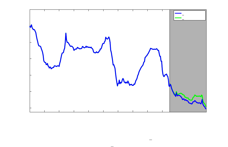
Figure 15: Shadow rates
1990 1992 1994 1996 1998 2000 2002 2004 2006 2008 2010 2012 2014
−2
0
2
4
6
8
10
r=0.25%
r estimated
Blue line: the shadow rate from the benchmark model with r = 0.25% in percentage points.
Green line: the shadow rate with estimated ˆr = 0.20% in percentage points. The gray area
marks the ZLB period from January 2009 to December 2013.
51

Figure 16: Liftoff dates
2009 2010 2011 2012 2013 2014
2010
2011
2012
2013
2014
2015
2016
r=0.25%
r estimated
Blue dots: lift-off dates from the benchmark model with r = 0.25%. Green stars: lift-off
dates with estimated ˆr = 0.20%. Black dashed line: the 45 degree line.
52

Table 1: Maximum likelihood estimates with robust standard errors
SRTSM GATSM
1200µ -0.3035 -0.2381 0.0253 -0.2296 -0.2069 0.0185
(0.1885) (0.1815) (0.0160) (0.1464) (0.1413) (0.0115)
ρ 0.9638 -0.0026 0.3445 0.9676 -0.0043 0.4854
(0.0199) (0.0183) (0.4821) (0.0184) (0.0200) (0.5408)
-0.0226 0.9420 1.0152 -0.0231 0.9333 1.0143
(0.0202) (0.0212) (0.5111) (0.0185) (0.0227) (0.5519)
0.0033 0.0028 0.8869 0.0030 0.0028 0.8935
(0.0018) (0.0019) (0.0385) (0.0015) (0.0020) (0.0423)
eig(ρ) 0.9832 0.9642 0.8452 0.9870 0.9627 0.8448
ρ
Q
0.9978 0 0 0.9967 0 0
(0.0003) (0.0003)
0 0.9502 1 0 0.9503 1
(0.0012) (0.0012)
0 0 0.9502 0 0 0.9503
(0.0012) (0.0012)
1200δ
0
13.3750 11.6760
(1.0551) (0.5591)
1200Σ 0.4160 0.4744
(0.0390) (0.0497)
-0.3999 0.2445 -0.4589 0.2175
(0.0369) (0.0233) (0.0447) (0.0188)
-0.0110 0.0033 0.0390 -0.0167 0.0013 0.0359
(0.0069) (0.0034) (0.0030) (0.0062) (0.0029) (0.0026)
1200
√
ω 0.0893 0.0927
(0.0027) (0.0027)
Log likelihood value 855.5743 755.4587
Maximum likelihood estimates for the three-factor SRTSM and the three-factor GATSM
with robust standard errors in parentheses. Sample: January 1990 to December 2013.
53

Table 2: Robustness check for structural break tests
p-value for ρ
xs
1
= ρ
xs
3
p-value for ρ
sx
1
= ρ
sx
3
Baseline 0.29 1.00
A1 estimate r 0.18 1.00
A2 2-factor SRTSM 0.13 0.97
A3 Fama-Bliss 0.38 1.00
A4 5-factor FAVAR 0.70 1.00
A5 6-lag FAVAR 0.09 0.98
7-lag FAVAR 0.19 0.97
12-lag FAVAR 0.22 1.00
This table consists of p-values for structural break tests with alternative model specifications.
54

Table 3: Forward guidance quotes
Date Quotes
12/16/2008 “ ...anticipates that weak economic conditions are likely to warrant excep-
tionally low levels of the federal funds rate for some time.”
03/18/2009 “...anticipates that economic conditions are likely to warrant exceptionally
low levels of the federal funds rate for an extended period.”
08/09/2011
∗
“...anticipates that economic conditions – including low rates of resource
utilization and a subdued outlook for inflation over the medium run – are
likely to warrant exceptionally low levels for the federal funds rate at least
through mid-2013 .”
01/25/2012
∗
“...decided today to keep the target range for the federal funds rate at 0 to
1/4 percent and currently anticipates that economic conditions – including
low rates of resource utilization and a subdued outlook for inflation over
the medium run – are likely to warrant exceptionally low levels for the
federal funds rate at least through late 2014 .”
09/13/2012
∗
“...decided today to keep the target range for the federal funds rate at 0 to
1/4 percent and currently anticipates that exceptionally low levels for the
federal funds rate are likely to be warranted at least through mid-2015 .”
12/12/2012 “...decided to keep the target range for the federal funds rate at 0 to 1/4
percent and currently anticipates that this exceptionally low range for the
federal funds rate will be appropriate at least as long as the unemploy-
ment rate remains above 6-1/2 percent, inflation between one and two
years ahead is projected to be no more than a half percentage point above
the Committee’s 2 percent longer-run goal, and longer-term inflation ex-
pectations continue to be well anchored.”
06/19/2013
∗
“...14 of 19 FOMC participants indicated that they expect the first increase
in the target for the federal funds rate to occur in 2015 , and one expected
the first increase to incur in 2016.”
12/18/2013 “...anticipates, based on its assessment of these factors, that it likely will
be appropriate to maintain the current target range for the federal funds
rate well past the time that the unemployment rate declines below 6-
1/2 percent, especially if projected inflation continues to run below the
Committee’s 2 percent longer-run goal.”
This table summarizes a list of forward guidance quotes, when the Fed expected a different
liftoff date or condition for the ZLB. All quotes except the one on 6/19/2013 are from
FOMC statements. The quote on 6/19/2013 is from Chairman Bernanke’s press conference.
Asterisks mark the statements with explicit lift-off dates, with the corresponding lift-off dates
in red.
Source: http://www.federalreserve.gov/monetarypolicy/fomccalendars.htm.
55
